| Issue |
A&A
Volume 627, July 2019
|
|
|---|---|---|
| Article Number | A65 | |
| Number of page(s) | 20 | |
| Section | Interstellar and circumstellar matter | |
| DOI | https://doi.org/10.1051/0004-6361/201935469 | |
| Published online | 01 July 2019 | |
Impact of nonconvergence and various approximations of the partition function on the molecular column densities in the interstellar medium★
1
Departamento Ciencias Integradas, Facultad de Ciencias Experimentales, Centro de Estudios Avanzados en Física, Matemáticas y Computación, Unidad Asociada GIFMAN, CSIC-UHU, Universidad de Huelva,
Spain
e-mail: This email address is being protected from spambots. You need JavaScript enabled to view it.
2
Instituto Universitario “Carlos I” de Física Teórica y Computacional, Universidad de Granada,
Granada,
Spain
3
INAF – Osservatorio Astrofisico di Arcetri,
Largo E. Fermi 5,
Firenze
50125, Italy
4
Université Grenoble Alpes, CNRS, IPAG,
38000
Grenoble,
France
5
Laboratoire Interuniversitaire des Systèmes Atmosphériques (LISA), UMR CNRS 7583, Université Paris-Est Créteil, Université de Paris, Institut Pierre Simon Laplace (IPSL),
Créteil, France
6
Department of Astronomy, University of Michigan,
311 West Hall, 1085 South University Avenue,
Ann Arbor,
MI 48109, USA
Received:
14
March
2019
Accepted:
28
May
2019
Abstract
We emphasize that the completeness of the partition function, that is, the use of a converged partition function at the typical temperature range of the survey, is very important to decrease the uncertainty on this quantity and thus to derive reliable interstellar molecular densities. In that context, we show how the use of different approximations for the rovibrational partition function together with some interpolation and/or extrapolation procedures may affect the estimate of the interstellar molecular column density. For that purpose, we apply the partition function calculations to astronomical observations performed with the IRAM-30 m telescope towards the NGC 7538–IRS1 source of two N-bearing molecules: isocyanic acid (HNCO, a quasilinear molecule) and methyl cyanide (CH3CN, a symmetric top molecule). The case of methyl formate (HCOOCH3), which is an asymmetric top O-bearing molecule containing an internal rotor is also discussed. Our analysis shows that the use of different partition function approximations leads to relative differences in the resulting column densities in the range 9–43%. Thus, we expect this work to be relevant for surveys of sources with temperatures higher than 300 K and to observations in the infrared.
Key words: techniques: spectroscopic / ISM: abundances / radio lines: ISM
Tables D.1–D.3 are only available at the CDS via anonymous ftp to cdsarc.u-strasbg.fr (130.79.128.5) or via http://cdsarc.u-strasbg.fr/viz-bin/qcat?J/A+A/627/A65
© M. Carvajal et al. 2019
 Open Access article, published by EDP Sciences, under the terms of the Creative Commons Attribution License (http://creativecommons.org/licenses/by/4.0), which permits unrestricted use, distribution, and reproduction in any medium, provided the original work is properly cited.
1 Introduction
Molecular astronomy needs accurate spectral analysis of the emission associated with various molecular species in order to identify them and to estimate the physical conditions of the interstellar region they are emitting from (Herbst & van Dishoeck 2009). A comprehensive molecular spectral characterisation is therefore extremely important for astrochemistry because the relative isotopic abundance estimates, the branching ratios, and the rate coefficients along with the activation energy of chemical reactions strongly relies on it (see Shaw 2006). In particular, a precise estimation of the column density of the molecular interstellar species is required in order to investigate the possible chemical reactions taking place in the interstellar medium (ISM). Such estimates are based on molecular spectroscopy that provides transition frequencies, line strengths, and partition functions for a given molecule through accurate laboratory spectral analyses.
Furthermore, the determination of ISM molecular and isotopic abundance ratios provides strong insight into the molecular formation mechanisms that occur in the ISM. To achieve this, it is necessary that the intensity calculation of the molecular species at different temperatures be reliable. It is important to note that the spectroscopic determination of the transition frequencies, the line strengths, and the partition function has to be very accurate due to the high spectral resolution that is now accessible with the present astronomical observatories.
The advent of new infrared and (sub-)millimeter observatories in the last decade (e.g., Atacama Large Millimeter Array (ALMA), Herschel, Stratospheric Observatory For Infrared Astronomy (SOFIA)) has motivated the molecular spectroscopy community to characterize increasingly complex molecules for which spectra were unrecorded until then. The spectroscopic data are gathered through intensive laboratory work, both experimental and theoretical, to predict new and accurate molecular data in the spectral range covered by the observational instruments. In addition, these data permit the exploration of new frequency ranges and enable the prediction of the frequencies via theoretical modeling.
Present databases compile and maintain the spectroscopic data updated in catalogs commonly used by the molecular astronomy community, such as the Cologne Database for Molecular Spectroscopy (CDMS)1 (Endres et al. 2016), the JPL (Jet propulsion Laboratory) database2 (Pickett et al. 1998), the Lovas/NIST catalog3 (Lovas 2004), the Toyama Microwave Atlas for spectroscopists and astronomers4, the SPLATALOGUE database5 (Remijan et al. 2007) and HITRAN6 (Gordon et al. 2017; Gamache et al. 2017). These databases have compiled a huge amount of data provided by spectral analyses performed via intensive laboratory spectral recordings.
So far, spectroscopic studies have made possible the identification of about 200 molecular species7 in star-forming regions and in the ISM. Nevertheless, for a number of molecular species, some reported physical quantities are not always normalized among the different authors. This is the case for example for the partition function values: there are several definitions of the nuclear spin statistical weight and the partition function is not always accounted for. This is also the case of the line strengths: some authors use a definition involving the square molecular dipole moment while others do not.
Moreover, the internal partition functions can be computed in different ways: a direct sum formula can be used, which involves the exponential of the energy levels, if those energy levels are known; if they are not known one can use various approximations to get the partition function. The main issue is the uncertainty on the partition function and its effect on molecular column densities. When the partition function is computed with the direct sum formula, sometimes it is provided without carrying out an appropriate convergence study in the temperature ranges of the ISM, typically from 9.375 to 300 K. The convergence on the partition function is said to be reached when a complete (full) list of rovibrational energy levels is available at the temperature of a given survey. In that case, due to the integrative nature of partition functions, completeness is more important in general than the accuracy with which those energy levels are estimated (Furtenbacher et al. 2016b). On the contrary, when the partition function is computed using various levels of approximations (because the energy level information is not or not easily available), large uncertainties on the partition function can also occur.
Molecular column densities (number of molecules per unit area along the line of sight, cm−2) are traditionally retrieved by a population rotational diagram (Mangum & Shirley 2015). Since the total molecular column density is proportional to the internal partition function, the uncertainties on the partition function will directly affect it. In particular, using an uncomplete (thus smaller) partition function will lead to underestimation of the molecular column densities and therefore some astrochemical conclusions could turn out to be slightly or even significantly different.
Mangum & Shirley (2015) published a review aimed at describing how to calculate the molecular column density from molecular spectral (rotational or ro-vibrational) transitions. Some years before, Fischer & Gamache (2002) and Fischer et al. (2003) studied, for atmospherical and astrophysical species, the convergence of the internal partition function. However, none of these former studies focused on the implications of using an approximate (or a not fully converged) partition function on the estimates of the interstellar molecular column densities.
The present paper aims at addressing the impact of different levels of approximations of the partition function on estimations of the interstellar molecular physical conditions. Some partition function interpolation and extrapolation procedures commonly used in the literature are also presented along with the analysis of their relevance regarding the temperature range. The interpolation and extrapolation procedures are indeed often used to determine the partition function value at any given ISM temperature. The effect of using an incomplete, that is, not fully converged, partition function is illustrated below via the use of the three following molecules, which represent different molecular geometries: isocyanic acid (HNCO), a quasilinear molecule; methyl cyanide (CH3 CN), a symmetric top molecule; and methyl formate (HCOOCH3), an asymmetric top molecule with a large amplitude internal rotor. Finally, a fourth molecule, hydrogen sulfide (H2 S), serves us to illustrate the effect of anharmonicity on the vibrational contribution of the partition function.
This paper is organized as follows: in Sect. 2 we briefly recall how to estimate the temperature and the interstellar molecular abundance from the molecular spectra under the assumption of local thermodynamic equilibrium (LTE). In Sect. 2 we highlight the need for a complete, that is to say a convergent, partition function to provide more accurate estimates and to decrease the uncertainties of the molecular column densities. In Sect. 3, we outline the various approximations that can be done for the rovibrational partition function calculation and the various interpolation and extrapolation procedures in terms of temperature. Section 4 describes the 30 m astronomical observations of NGC 7538-IRS1. In Sect. 5, we give examples of derived molecular column density estimates from different partition function approximations or interpolation and extrapolation procedures. Finally, the conclusions are set out in Sect. 6.
2 Relevance of a suitable partition function convergence study in the rotational temperature diagram estimates
In this section, we briefly describe how the ISM molecular column densities and/or abundances are derived. For emission lines associated with a given molecule in an astronomical survey, one can derive the total molecular column density N as a function of the integrated intensity W, the partition function and the excitation temperature. The mathematical expression depends on the assumption considered (i.e., optically thin emission, negligible background temperature, LTE, and so on; for further details see Goldsmith & Langer 1999; Mangum & Shirley 2015).
We therefore assume that LTE is reached and the excitation temperature will be given by the quantity T. Hence, in absence of collision rates, the upper energy state column density, Nu, can be related to the total column density, N, of the molecule by
 (1)
(1)
where k is the Boltzmann constant, Q(T) is the molecular partition function, and gu and Eu are the degeneracy and the energy for the upper level u involved in the molecular transition, respectively. The degeneracy for the upper level involved in the transition gu can be given as
 (2)
(2)
where Ju is the upper state rotational angular momentum and  is the nuclear spin statistical weight of the upper state.
The total molecular column density N of a molecular species, which is related to the upper energy state column density Nu by Eq. (1), and the rotational temperature T can be given by (Goldsmith & Langer 1999):
![Mathematical equation: \begin{equation*}\ln \left[\frac{3 \, k \, W}{8 \, \pi^3 \, \nu \, S\mu^2 \, g_{\textrm{u}}} \right]= \ln \left[\frac{N}{Q(T)}\right] - \frac{E_{\textrm{u}} }{k \, T}, \end{equation*}](/articles/aa/full_html/2019/07/aa35469-19/aa35469-19-eq4.png) (3)
(3)
![Mathematical equation: \begin{equation*}\ln \left[\frac{8 \, \pi \, k \, \nu^2 \, W}{g_{\textrm{u}} \, h \, c^3 \, A_{\textrm{ul}}} \right]= \ln \left[\frac{N}{Q(T)}\right] - \frac{E_{\textrm{u}} }{k \, T}, \end{equation*}](/articles/aa/full_html/2019/07/aa35469-19/aa35469-19-eq5.png) (4)
(4)
where h is the Planck constant and c is the speed of light in vacuum. In the above equations the integrated intensity W, given in K km s−1, and transition frequency ν for a given line are provided through the spectral interstellar observations, and therefore their accuracies are limited by observational constraints. The line strength Sμ2 or the Einstein coefficient Aul for spontaneous emission, the upper state energy Eu and the molecular partition function Q(T), are all predicted after the spectral characterization of the molecule is performed. Therefore, their accuracies are also limited by the calculation and prediction error bars based on laboratory work.
To determine the column density N and the temperature T from the observations, a linear regression, so-called rotational temperature diagram, is carried out after substitutingin Eq. (3) (i) the data for the detected lines from the observational survey namely W and ν, and (ii) the spectroscopic data of the molecules: Sμ2, gu, Eu, and Q(T).
The linear regression of Eq. (3) provides the y-intercept, which corresponds to b = ln (N∕Q), and the slope which is related to the inverse of temperature by a = −1∕T (Turner 1991). Therefore, the excitation temperature can easily be estimated from the slope whereas the total molecular column density N is obtained from the y-intercept provided that the molecular partition function is known. This means that the molecular partition function values at a characteristic temperature range directly affect the value of N. This is why a detailed convergence study of the molecular partition function is relevant to obtain a correct estimate of N.
For instance, if the source under study is a hot region where excited vibrational states of a given molecule are populated (T ≥ 300 K) and if the molecular partition function is computed only taking into account the rotational structure of the molecule (i.e., in its vibrational ground state), the resulting molecular column density will be underestimated. Therefore, for high-temperature regions, the rotational temperature diagrams should contain both the rotational and vibrational contributions and, therefore a more accurate designation for them should be rovibrational temperature diagrams rather than rotational temperature diagrams, which is a slightly misleading term in some cases.
In Sect. 4, the rovibrational temperature diagrams for CH3 CN, HNCO, and HCOOCH3 resulting from our observations are given as examples.
3 Molecular partition function
In this section, we present some approximations used for the calculation of the rovibrational partition function of a free molecule with the aim of reaching the correct values (under a convergence study) at the typical temperature range of the ISM.
A molecular partition function8 is defined as a direct sum of exponential terms that involve the energy levels and the temperature of the environment where the molecule is located. Therefore, the direct sum of the partition function can be given as
 (5)
(5)
where Ji and  are the rotational angular momentum and the nuclear spin degeneracy of the energy level i, respectively, and Ei is the rovibrational energy usually referred to the ground vibrational state as it is assumed that uniquely the ground electronic state is populated (Fischer & Gamache 2002; Cerezo et al. 2014). This means that an accurate partition function will be determined at any temperature if all energies Ei are accurately known. At the present time, this is unfortunately often not possible because all transitions (and thus all energy levels) have not yet been measured. From a quantum mechanical point of view, one might assume that the molecular parameters derived from the observed transition frequencies can be used to predict the missing energy levels, however their estimates are not always lyingwithin the experimental uncertainty. Therefore, the exponential terms in Eq. (5) are limited to the lowest energies Ei up to a certain upper threshold.
The energy threshold is selected depending on the environment under study, for example, ISM or planetary atmospheres, which correspond to given temperature ranges. Regarding the number of exponential terms in Eq. (5), once the numerator Ei is large in comparison with the denominator kT, the exponential  can be neglected as long as Ei reaches a certain upper threshold. This means that according to the temperature of the environment, the upper threshold energy can be selected so that the direct sum in Eq. (5) uses a complete set of rovibrational energy levels and therefore reaches convergence (Fischer & Gamache 2002).
In general, when the energy levels do not appear in a database or in the literature, or cannot be calculated easily, approximations are usually considered for determining the molecular partition function. In the case of the C2 molecule, the internal partition function is computed via the direct sum formula using a combination of experimental and theoreticallyderived energy levels (Furtenbacher et al. 2016a). The theoretical treatment allows the authors to obtain a full set of energies for the nine electronic states considered during the determination of the ideal-gas thermochemistry of C2. However, those theoretically derived rovibronic levels are complete but of limited accuracy. The sources of inaccuracies and uncertainties in the partition function are fully discussed in this paper. Unfortunately this is not always the case in the literature. We investigate here the particular case of molecules that possess one large amplitude torsional mode arising from a CH3 top. In that instance, Ei stands for the vibrational-torsional-rotational energy (also referred to as the vibrational-torsional ground state) and the partition function can be approximated as a product of the rotational contribution Qrot (T), the torsional Qtor (T), and the vibrational Qvib (T), (Herzberg 1991), assuming that the torsional-vibrational-rotational coupling interactions in the Hamiltonian can be left out:
 (6)
(6)
In this case, for some isotopologs of methyl formate, Favre et al. (2014) assessed that Eq. (6) is a good approximation for temperatures under 300 K.
If the molecule has no torsional mode, the torsional contribution Qtor is simply omitted in Eq. (6).
3.1 Rotational partition function
The rotational partition function Qrot(T) (e.g., Herzberg 1991; Groner et al. 2007) can be written as a direct sum,
 (7)
(7)
where  represents the energy for the ith rotational state. The degeneracy
  is included in the definition of the rotational contribution of the partition function (Eq. (7)) because in general
  is associated with the K degeneracy of the symmetric top (or Ka and Kc for asymmetric top; see Sect. 3.4). In the present paper we address the special case of symmetric (or asymmetric) tops where the degeneracy is state independent, meaning that
  .
.
The classical approximation of the rotational partition function (Eq. (7)), based on a rigid rotor model, can also be used for symmetric and slightly asymmetric tops considering the rotational constants defined in the Principal Axis System (McDowell 1990; Herzberg 1991; Mangum & Shirley 2015).
3.2 Vibrational partition function
The vibrational partition function Qvib(T), which only takes into consideration the small amplitude vibrational modes, can be computed using the harmonic approximation (Herzberg 1991):
 (8)
(8)
where Nvib and  represent the number of the small-amplitude vibrational modes and their fundamental energies, respectively. This approximation is a good alternative to the direct sum expression of the vibrational partition function for the ISM temperatures for the following reasons. In general, the energy values of the fundamental vibrational states are known but only a handful of excited term values are determined. Furthermore, the limited number of known excited terms is not considered, and as a consequence the exponential terms have larger
  with respect to the typical ISM temperatures (100–200 K). More specifically, the terms with large fractions of
  can be neglected in the calculation of the vibrational partition function. Finally, the convergence of the vibrational partition function can be generally reached only using the lowest vibrational energies.
However, two comments on Eq. (8) need to be added. First, it is known that the vibrational anharmonicity affects, in general, the vibrational energy structure of floppy or semi-floppy molecules, mainly the excited vibrational levels, by decreasing the vibrational term values  with respectto their harmonic values. Therefore, by including the anharmonicity, the direct sum of the vibrational partition function increases (Zheng et al. 2012; Skouteris et al. 2016). Second, molecules can undergo strong vibrational resonances such as the Fermi and Darling-Dennison interactions (Herzberg 1991), which perturb the energy levels (sometimes by hundreds of cm−1). These perturbation effects are not reflected in the fundamental energies used in Eq. (8).
Therefore, it is worthwhile to test whether the harmonic expression for the vibrational partition function of Eq. (8) is a good approximation of the direct sum, as Furtenbacher et al. (2016b) did in a comprehensive study of the rovibrational partition function for water molecules. In order to assess the deviation of the harmonic partition function with respect to the direct sum, we therefore chose the hydrogen sulfide molecule H2 S because: (i) this molecule has strong Fermi and Darling-Dennison interactions and large anharmonic effects in the vibrational degrees of freedom; and (ii) a huge amount of compiled experimental and predicted vibrational levels (204 vibrational term values in total up to approximately 17 000 cm−1) are available (Carvajal & Lemus 2015). Therefore, H2S is a good molecule to test the effect of the anharmonicity on the partition function because concerning the term values of its vibrational levels we can increase the temperature high enough to compare the direct sum with the harmonic approximation. Taking into account the vibrational levels of H2S we calculate the values of the vibrational partition function contribution by direct sum. At T = 1000 and 2000 K the resulting values of the direct sum are 1.28309 and 2.45873, respectively,and the relative differences with the harmonic approximation calculated from Eq. (8) are of 0.13 and 1.34%, respectively. Therefore, we expect that within the typical ISM temperatures, which are lower than the two temperatures given above, the harmonic vibrational partition function expression can in general be considered as a good approximation.
3.3 Torsional partition function
In the particular case of molecules with one large-amplitude torsional CH3 top, the torsional contribution to the partition function Qtor(T) can be computed by the direct sum (Favre et al. 2014):
 (9)
(9)
where E(tor)(vt, A) and E(tor)(vt, E) are the torsional substate energies for the A (either A1 or A2) and E symmetries (according to the molecular symmetry group  ), respectively, relative to the torsional vt = 0 ground state, that is, E(tor)(vt = 0, A) = 0 cm−1.
Different approximations for the torsional partition sum can be considered in terms of the selection of the maximum torsional quantum number  . For the particular case of methyl formate isotopologs, the convergence is achieved within 1% when
  for a temperature range up to T = 300 K (see Tables 9 and 10 of Favre et al. 2014). However, as the convergence of Eq. (9) depends on the torsional term values, which are specific to each molecule, and on the temperature, it is recommended whenever possible to perform a convergence test of the values obtained for the partition function from the direct sum by simply increasing vt and adding the corresponding energies in the partition function until a negligible change of its value occurs.
For molecules with two or more large-amplitude torsional CH3 tops, the number of exponential terms in Eq. (9) should be extended to all torsional substates for a given torsional quantum number vt.
3.4 Nuclear spin statistical weights
The nuclear spin statistical weight gns can be computed according to Bunker & Jensen (1989). A complete description of the calculation can be found in this latter reference, and so we only summarize it here. The nuclear spin statistical weight is obtained taking into account that the sign of the complete internal wavefunction9 either changes or is kept invariant under the odd molecular symmetry group permutations of identical nuclei with half-integer spin (so-called fermions) or with integer spin (named bosons), respectively. For both cases however, the parity of the complete internal wavefunction can be positive or negative under the symmetry group inversion action (Bunker & Jensen 1989).
Since the complete internal wavefunction with symmetry Γint can be written as the product of the rovibronic function, with symmetry Γrve, and the nuclear spin function, with symmetry Γns, the following relationship exists among the various symmetry representations: Γint ⊂ Γrve ⊗ Γns. Therefore, the spin statistical weight gns is the number of complete internal wavefunctions of the allowed Γint symmetry that can originate from a given Γrve (Bunker & Jensen 1989).
In general, gns is split into the reduced nuclear spin weight gI and the K-level degeneracy gK (Turner 1991; Mangum & Shirley 2015) as follows:
 (10)
(10)
A possible source of error could come from the fact that the left part of Eq. (3), ![Mathematical equation: $\ln \left[\frac{3 \, k \, W}{8 \, \pi^3 \, \nu \, S\mu^2 \, g_{\textrm{u}}} \right]$](/articles/aa/full_html/2019/07/aa35469-19/aa35469-19-eq25.png) , contains the statistical weight of the upper state, but at the same time the right part of Eq. (3) contains the partition function Q(T), which also depends on the statistical weight. Inconsistencies and errors therefore occur when taking from the literature a value for the partition function Q(T) (where the statistical weight gns is calculated in one way), and then another value for the upper level degeneracy gu (linked to gI gK through Eq. (2)) calculated in another way. Of course, this source of error can easily be resolved if the values of gns are reported apart from the rest of the partition function, allowing the users to carefully check the values of gns and gu before considering the partition function in Eq. (3).
, contains the statistical weight of the upper state, but at the same time the right part of Eq. (3) contains the partition function Q(T), which also depends on the statistical weight. Inconsistencies and errors therefore occur when taking from the literature a value for the partition function Q(T) (where the statistical weight gns is calculated in one way), and then another value for the upper level degeneracy gu (linked to gI gK through Eq. (2)) calculated in another way. Of course, this source of error can easily be resolved if the values of gns are reported apart from the rest of the partition function, allowing the users to carefully check the values of gns and gu before considering the partition function in Eq. (3).
3.5 Interpolation and extrapolation
Whenever possible, the best procedure is to calculate the direct sum using Eq. (5) after making sure that the sum reaches convergence for the temperature under study. This of course may not be always possible since it requires a rather precise knowledge of the vibrational, rotational, and torsional (if large amplitude torsional motion(s) is involved) energies. Furthermore, depending on the temperatures studied, those energy levels may not be available through experimental transition measurements or even through calculated transitions. In those cases, the partition function can alternatively be tabulated, within a given temperature range, via fitted mathematical parameters using different power expansions depending on the temperature (Irwin 1981; Fischer & Gamache 2002; Barton et al. 2014). These power expansions, apart from being used as a simple way of storing or computing the rotational-vibrational-torsional partition functions, are useful to interpolate and/or extrapolate the partition function values to the temperature of any ISM region, and they are therefore often used. Nevertheless, the main advantage of the tabulation of the partition function is due to the fact that in general onlya set of partition function values are reported for a set of temperatures (typically from 2.725 up to 500 K) and the direct sum cannot be obtained if the rovibrational energies are not available, as is usually the case.
In Sect. 3.6 we consider three molecular species as examples to analyze the suitability of the most used procedures according to the ISM temperature range. This analysis led us to draw the conclusion that a noteworthy difference of around 10% can be attributed to using one or another interpolation procedure. Two main interpolation procedures can be distinguished: the linear interpolation, which is obtained by simply taking two values of the partition function at two successive temperatures and tracing a straight line between them (which of course is strictly valid only between the two points), and the nonlinear interpolation, which uses the power expansions of the rotational-vibrational-torsional partition function in terms of temperature.
As far as the nonlinear power expansions in the temperature are concerned, two kinds of methods are found in the literature. One method was considered by Fischer & Gamache (2002), who used a fourth-order polynomial of Q(T) in terms of temperature T, and is valid for a temperature range from 70 to 300 K:
 (11)
(11)
In the present study, a polynomial extended up to sixth order is considered, where seven parameters are fitted from the computed partition function values. In the second method, a nonlinear fit of a power expansion of log10(Q) in terms of the log10(T) is also found in the literature (Irwin 1981; Barton et al. 2014), as follows:
 (12)
(12)
where seven parameters are also fitted.
It is important to note that in comparison to the linear interpolation, Eqs. (11) and (12) can be successfully used to interpolate the partition function along the whole temperature interval for which they were fitted, and in addition to extrapolate them to further values of the temperature interval used in the fitting.
Furthermore, we note that one can also use the rigid rotor approximation of Herzberg (1991) for symmetric and asymmetric tops, respectively, to derive the rotational partition function at any temperature T, using the value of the partition function at T = 300 K as a benchmark:
 (13)
(13)
A quantitative example of the extrapolation function (Eq. (13)) is given in Sect. 3.6.3.
3.6 Example of molecular partition function calculation
In this section we discuss the calculation of the partition functions for the three following molecules that represent different geometries: isocyanic acid (HNCO), which is a quasilinear molecule, methyl cyanide (CH3CN), a symmetric top molecule, and methyl formate (HCOOCH3), an asymmetric top molecule which in addition has a large-amplitude internal rotor from CH3 top. The nuclear spin statistics and the nonlinear polynomial expansions of the partition functions are discussed in Appendices A and B, respectively.
Rotational partition function for isocyanic acid (HNCO).
3.6.1 Isocyanic acid (HNCO)
Isocyanic acid is a slightly asymmetric prolate rotor (Niedenhoff et al. 1995). The shortage of spectral data from the different vibrational bands does not allow us to obtain the partition function straightforwardly from Eq. (5) as far as the vibrational energies are concerned. Nevertheless, there are enough rotational levels that can be deduced from measured transitions (Kukolich et al. 1971; Hocking et al. 1975; Niedenhoff et al. 1995; Lapinov et al. 2007). Moreover, fundamental vibrational term values were already recorded in the gas phase (East et al. 1993) so one can compute the partition function using Eq. (6). The torsional term is not considered at all because this motion does not occur in HNCO.
In Table 1 we compare the values of the rotational partition function for different temperatures ( in the second column) using the approximation for slightly asymmetric tops (McDowell 1990) with the value of the rotational partition function computed as a direct sum of the predicted rotational energy levels up to J = 135 and Ka = 30 (Lapinov et al. 2007)using Eq. (7) without considering the nuclear spin statistical weight (Qrot(direct sum) in the third column). It is clear from Table 1 that the approximation of McDowell (1990) or similar approximations are far from being satisfactory at temperatures lower than 20 K.
As far as the vibrational contribution of the partition function is concerned, there are not enough observed or computed vibrational energies available to compute the direct sum. One needs to use the harmonic approximation of the vibrational partition function from Eq. (8). In Table 2, the values of the harmonic approximation of the vibrational partition function  from Eq. (8) are multiplied by the rotational partition function to obtain the rotation-vibration partition function
  for the isocyanic acid (HNCO) molecule in the temperature range from 2.725 to 500 K. The values of the rovibrational contribution from the present study are compared with those coming from the CDMS catalog Q(CDMS) which considers only the rotational partition function as a direct sum and no vibrational contribution. It is notable that here the vibrational contribution is becoming significant at temperatures higher than 225 K. Therefore, if the molecule emits in the ISM object at a temperature greater than 200 K, it is advisable to consider the vibrational contribution in the calculation of the molecular partition function.
The relative differences of Qrv(Present work) with respect to Q(CDMS) are in general larger than the uncertainties of Qrv(Present work). An upward estimate of its uncertainty has been provided in Table 2 considering large uncertainties of 100 MHz and 1 cm−1 for the rotational energies and the vibrational fundamentals, respectively. We have also computed the uncertainty of the Qrv (Present work) values using the uncertainties for each rotational energy level (Pickett 1991), but these are even smaller.
In Table D.1 (available at the CDS), the computed rotational, vibrational, and rovibrational partition function Qrv (Present work) for isocyanic acid (HNCO) are also given up to T = 500 K in intervals of 1 K.
3.6.2 Methyl cyanide (CH3CN)
Methyl cyanide, also named acetonitrile, is a symmetric rotor very close to the prolate limit (Müller et al. 2015). As for isocyanic acid, the partition function can be calculated through Eq. (6) after computing the rotational partition function and the vibrational contribution separately. There is no torsional contribution. The rotational energy data were taken from Kukolich et al. (1973), Boucher et al. (1977), Kukolich (1982), Cazzoli & Puzzarini (2006), and Müller et al. (2009) while the vibrational fundamental frequencies come from Rinsland et al. (2008).
In Table 3, the classical approximation of the rotational partition function (using McDowell 1990) is compared for CH3CN to the direct sum expression for the rotational partition function (Eq. (7)) but omitting the nuclear spin weight. The classical approximation has been computed using the rotational constants from Müller et al. (2015) while the direct sum has been computed for all the rotational energy levels up to J = 99 (Müller et al. 2009). It can be noted that the classical approximation for the rotational partition function contribution is not accurate enough for temperatures lower than 5 K. Hence, in the present study, the rovibrational partition function has been calculated as the product of the direct sum of the rotational contribution and the harmonic vibrational approximation (see Table 2).
In Table 2, the values of the rovibrational partition function  are given from 2.725 to 500 K (Col. 3) and are compared with the rovibrational partition function provided by the CDMS catalog (Col. 4; Endres et al. 2016); the vibrational partition function contribution of this catalog only takes into consideration the vibrational fundamentals up to about 1200 cm−1. For comparison purposes, the nuclear spin statistical weight has been suppressed in both contributions. It can be noted in Table 2 that they disagree at temperatures lower than 20 K and larger than 300 K. At temperatures below 20 K the discrepancy, which could only stem from the rotational partition function, could come from an extra contribution overlooked in the instructions since the completeness of the rotational partition function calculated in the present study has also been proven by the good agreement obtained with the rotational contribution computed by Rinsland et al. (2008). For the highest temperatures, the difference between these two calculations (CDMS vs. this work) only comes from the vibrational contribution of the partition function, which starts to become significant for temperatures above 300 K.
The uncertainties of Qrv(Present work) are also given in Table 2. They are rather small despite them being estimated upwards considering large rotational energy uncertainties of 100 MHz and of 1 cm−1 for the vibrational fundamentals. In a temperature range above 20 K, the uncertainties of Qrv (Present work) are significantly smaller than the relative differences with respect to Q(CDMS).
In Table D.2 (available at the CDS), the rotational, vibrational, and rovibrational partition functions calculated in the present study for methyl cyanide (CH3CN) are provided in intervals of 1K up to T = 500 K.
Vibrational and rotational-vibrational partition function for methyl cyanide (CH3 CN) and isocyanicacid (HNCO).
Rotational partition function for methyl cyanide (CH3CN).
3.6.3 Methyl formate (HCOOCH3)
Methyl formate is an asymmetric near-prolate rotor which has a large-amplitude motion due to the torsion of the methyl group. As a consequence, each rotational line is split into a doublet characterized by the symmetry labels A1 or A2 and E (Carvajal et al. 2007), respectively.Therefore, for this molecular species, the torsional contribution has to be taken into account in the approximated expression of the partition function (Eq. (6)). Other species of astrophysical interest undergoing a large-amplitude motion of the methyl group CH3 are, for example, methanol and acetaldehyde (Voronkov et al. 2002; Martín et al. 2006; Xu et al. 2008, 2014; Wang et al. 2011; Slocum et al. 2015; Pearson et al. 2015; Kleiner et al. 1996, 1999, 2008; Elkeurti et al. 2010; Smirnov et al. 2014; Margulès et al. 2015; Codella et al. 2016; Zaleski et al. 2017).
A number of spectroscopic studies have been carried out for the identification of the isotopologs of methyl formate in the ISM (Carvajal et al. 2009; Margulès et al. 2010; Takano et al. 2012; Tercero et al. 2012; Favre et al. 2011, 2014; Haykal et al. 2014). The spectral analyses were focusing on the rotational features of these molecular species mainly in the ground and first torsional excited states (Curl 1959; Brown et al. 1975; Bauder 1979; Demaison et al. 1983; Plummer et al. 1984, 1986; Oesterling et al. 1999; Karakawa et al. 2001; Odashima et al. 2003; Ogata et al. 2004; Willaert et al. 2006; Carvajal et al. 2007, 2010; Maeda et al. 2008b; Ilyushin et al. 2009; Tudorie et al. 2012; Duan et al. 2015) while the other vibrational bands were in general not considered except in a few cases (Maeda et al. 2008a; Kobayashi et al. 2013, 2018).
A significant achievement was when the lowest torsional-rotational transitions for internal rotors could be reproduced and predicted using the so-called Global Approach, where the torsion-rotation Hamiltonian matrix (containing higher-order terms describing the coupling between rotation and torsion) is set up in an extended basis set containing the nine lowest torsional vt states. By fitting vt = 0 and 1 bands within experimental-accuracy laboratory data, Tudorie et al. (2012) provided a set of 53 parameters with a weighted (unitless) root-mean-squared deviation of 0.67. Even though the experimental data only included vt = 0 and 1, the fitted parameters contain implicitly all the interactions involving vt < 9. Predicted energy levels higher than vt = 1 can therefore in principle be computed using those parameters but care has to be applied as the extrapolation to higher torsional levels lacks accuracy as they are not based on experimentally fitted parameters.
Therefore, a rotational-torsional-vibrational partition function can only be computed in an approximated way. The vibrational contribution was obtained via the harmonic approximation formula (Eq. (8)) by using experimental vibrational fundamental frequencies provided by Chao et al. (1986), while the rotational and torsional contributions were obtained by performing a direct sum on the predicted energies.
Comparison of rotational and rotational-vibrational-torsional partition functions
It is worth noting that the most extensive rotational-torsional partition function calculation of methyl formate was provided by Tudorie et al. (2012) although this calculation was restricted to temperatures from 100 to 300 K in steps of 10 K. This partition function was computed as a direct sum of the predicted rotational-torsional energies calculated using the Hamiltonian parameters obtained in a fit of observed transition lines in the ground and first excited torsional vt = 0 and 1 states. The vibrational partition function was not provided in Tudorie et al. (2012).
In 2014, Favre et al. (2014) provided rotational-torsional-vibrational partition function values for methyl formate in the temperature range from 9.375 to 300 K after a comprehensive convergence study was carried out. More specifically, the partition function was computed using Eq. (6). The rotational contribution was calculated as a direct sum (Eq. (7)) for the rotational-torsional energies with torsional quantum number vt = 0 and A1 or A2 symmetries up to J = 79. The torsional (corresponding to the large-amplitude motion) contribution was calculated as a direct sum by Favre et al. (2014) using Eq. (9) up to  and the following torsional energies: (i) for the torsional levels vt = 0 to vt = 2, from the measured and predicted transitions coming from Ilyushin et al. (2009), (ii) for the levels vt = 3 to vt = 4, ab initio torsional term values were used (Senent et al. 2005), and (iii) for the levels vt = 5 to vt = 6 a harmonic estimation from those torsional levels were used. The vibrational contribution of the small-amplitude vibrations was obtained using the harmonic approximation (Eq. (8)).
In the present study, the calculation of the rotational-torsional-vibrational partition function is revisited. The values obtained between 9.375 and 300 K by Favre et al. (2014) are extended here from 2.725 to 500 K. Despite the fact that the partition function of Favre et al. (2014) provided good agreement with respect to that given by Tudorie et al. (2012), it is expected that our present study gives more accurate partition function values mainly because of the increase of the maximum torsional quantum number  in Eq. (9), as described below.
Favre et al. (2014) verified that, for methyl formate, the classical approximation (Herzberg 1991) of the rotational partition function provided satisfactory results compared to its direct sum expression for rotational energies up to J = 79 and for a temperature range from 9.375 to 300 K. Table 4 shows that the classical approximation for methyl formate is fairly good even for low temperatures around 2.725 K. In fact, the comparison of the values provided by the direct sum and the classical expression represents a good validation of the convergence reached by the rotational contribution of the partition function in the temperature range up to 500 K.
To extend the torsional contribution of the partition function at temperatures from 300 to 500 K, we used Eq. (9) with torsional states up to  . The torsional energies up to vt = 4 were predicted from our internal rotation software BELGI (Kleiner 2010) using the Hamiltonian parameters experimentally fitted by Tudorie et al. (2012). The torsional energy levels from vt = 5 to vt = 10 were estimated with a harmonic approximation. Although it is known that the harmonic energy estimate provides a smaller value for the torsional partition function, in comparison with the one obtained when all the experimental torsional levels are available, this approximation is still justified for methyl formate and provides a minimum threshold for the torsional partition function values at high temperatures. Indeed, as mentioned above, the higher excited torsional energies can only be extrapolated from the experimentally deduced parameters of the Hamiltonian from observed transitions within vt = 0 and 1.
In Table 5, the torsional partition function calculated as a direct sum in the present study are given for various  equal to 4, 6, 8, and 10. We can make one comment about the fact that Favre et al. (2014) presented the cutoff at
  for temperatures up to 300 K. In fact, the deviation between
  and
and  approximations is smaller than1%, and between
  and
and  it is of 0.22% at T = 300 K. Therefore, the convergence at T = 300 K can be considered as accomplished. However, at T = 500 K, the difference in extending the calculation of the torsional partition function from
  to
to  is still 3.6%. Extending the calculation from
  up to
up to  torsional levels produces a difference in the torsional partition function of 1.6% at T = 500 K. For completeness, Table 5 also gives the harmonic approximation of the vibrational (for the modes other than the torsional mode) contribution of the partition function.
The rotational-torsion-vibrational partition function values obtained in the present study as the product of the rotational, torsional, and vibrational contributions (Eq. (6)) are given in the third column of Table 6 for a temperature range from 2.725 to 500 K and are compared to the values of Favre et al. (2014) up to 300 K. The differences between the present study and the values of Favre et al. (2014) are very small but increase with temperature. A conservative estimate of the uncertainty of Qrvt(Present work) has also been provided, considering the rotational energy uncertainties of 100 MHz, the uncertainties of the vibrational fundamentals as 1 cm−1 and the uncertainties of the torsionalenergies as 0.01 cm−1 for vt = 0 and 1, 1 cm−1 for vt = 2 states, 5 cm−1 for vt = 3 and 4, and 20 cm−1 for the remainder (vt = 5–10). Despite the upward estimate of the uncertainties, they are smaller than 0.5% of the partition function value.
Finally, we note that for T = 500 K we used the rotational partition function value given by the classical approximation (Herzberg 1991). This is justified because the relative difference between the direct sum and the approximated rotational partition function tends to decrease with temperature (see Table 4). Indeed, for temperatures higher than 330 K, the direct sum expression does not reach the convergence if the sum is limited to rotational energy levels up to J = 79, which is the limit where we measured and fit the experimental data (Kleiner 2010).
In Table D.3 (available at the CDS), the values of the rotational, torsional, vibrational, and rotational-torsional-vibrational partition function computed in the present study for methyl formate are provided up to T = 500 K using an interval of 1 K.
In Fig. 1, the partition function for the main isotopolog of methyl formate computed in the present study and the one published in the JPL catalog are compared by considering gns = 1 in both cases. The partition function of the present study was extended up to T = 500 K and is plotted as full red circles. The JPL partition function is displayed in full green squares. The JPL values were computed as a direct sum (Eq. (5)) of all the predicted rotational-torsional energies with rotational angular momentum up to J = 109 and including the ground and first torsional levels vt = 0 and 1 (Ilyushin et al. 2009). The JPL values (Pickett et al. 1998) were given in the typical set of temperatures reported in the astronomical catalogs, that is, T = 9.375, 18.75, 37.50, 75.0, 150.0, 225.0, and 300.0 K.
Figure 1 shows that the partition function deviations between the present study and the JPL catalog values start to be important at T ≥ 150 K. Indeed, at T = 150 K, they differ by about 20% while at T = 225 K and T = 300 K the deviations are ~43 and ~61%, respectively.These differences are due to the fact that the JPL partition function does not include the vibrational contribution and takes into account the torsional contribution only up to vt = 0 and 1, whereas our calculation includes torsional levels up to vt = 10 as well as the vibrational contribution.
Rotational partition function for methyl formate (HCOOCH3).
Torsional(a) and vibrational contributions of the partition function for methyl formate (HCOOCH3).
Rotational-torsional-vibrational partition function (a) for main isotopolog of methyl formate (H12COO12CH3).
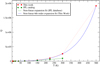 |
Fig. 1 Convergence study of the partition function for methyl formate. Comparison of the partition function values computed in the present study (full red circles) and JPL database (full green squares). The linear interpolation of the partition function computed in the present study is given as red dashed lines while the nonlinear sixth-order polynomial fit is given as a blue line. From JPL, the linear interpolation and the nonlinear fit (green line) are apparently overlapped. The differences between the two partition functions are due to the fact that the JPL partition function does not include the vibrational contribution and does take into account the torsional contribution from Eq. (9) only up to vt = 0 and 1, whereas we are including torsional levels up to vt = 10 as well as the vibrational contribution. |
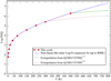 |
Fig. 2 Logarithm of Q in base 10 is provided according to calculation of the present study (full red circles). The nonlinear sixth-order decimal logarithm polynomial curve fitting (blue line) is provided up to T = 800 K. This result is compared with the extrapolated values obtained using the partition function at T = 300 K as benchmark (brown line) (see Eq. (13)). In addition, it has been included the extrapolated values computed with Eq. (13) but using T = 500 K as benchmark (green line). |
Comparison of partition functions from nonlinear polynomial expansions and direct sums
In order to better assess the rotational-vibrational-torsional partition function obtained at the estimated temperature of the ISM survey from the linear and nonlinear interpolation procedures (see Appendix B), we plot the values of Q against the temperature in Fig. 1. The results of the linear interpolation (traced as a straight line by considering the sets of two adjacent partition function points) and those from the nonlinear interpolation fitting (in this case the sixth-order polynomial expansion, from Eq. (11)) are also displayed. It is immediately apparent that the computed partition function values show a better agreement with the nonlinear interpolation (third column of Table 6) than the linearly interpolated partition function values. In fact, the linear interpolation provides overestimated values for the partition function (which become even larger for higher temperatures). Therefore, using a linear interpolation of the partition function will lead to overestimation of the molecular column density according to Eqs. (3) and (4).
Figure 2 shows the log10(Q) values computed in the present study with respect to the temperature from T = 2.725 K up to 500 K (red full circles). The nonlinear curve fit, displayed in this figure as a blue continuous line, is the sixth-order decimal logarithm polynomial expansion (Eq. (12)). The latter was used to extrapolate the partition function to temperatures from 500 to 800 K. It is immediately apparent that up to the temperature of 800 K, the polynomial expansion follows the same trend as the lower temperatures partition function. In addition, the values that have been extrapolated via the polynomial expansions are consistent with the present partition function values computed using the direct sum between 2.725 and 500 K.
Finally, the extrapolation carried out with the sixth-order decimal logarithm polynomial expansion (Eq. (12)) are compared with the extrapolated values obtained using the partition function at T = 300 K (brown line) and T = 500 K (green line) using the expression of Eq. (13). This leads us to conclude that for methyl formate the nonlinear fitting expression is more suitable in the extrapolation procedure of the partition function values.
4 A test case: observations of HNCO, CH3CN, and HCOOCH3 towards the star forming region NGC7538–IRS1
4.1 Observations
Observations of NGC 7538–IRS1 were carried out with the IRAM 30 m telescope at Pico Veleta in Spain on 2013 December 5, 6, and 10. The observations were performed in the “position switching” mode, using [−600′′,0′′] as referencefor the OFF position, toward a single pointing (αJ2000 = 23h13m45. s5, δJ2000 = +61°28′12.′′0). The E230 EMIR receiver was used in connection with the 200 kHz Fourier transform spectrometer (FTS) backend in the frequency ranges 212.6–220.4, 228.3–236.0, 243.5–251.3, 251.5–259.3, 259.3–267.0, and 267.2–274.9 GHz. The half-power beam size is 10′′ for observations at 250 GHz. The vLSR was −57 km s−1 and the spectral resolution is about 1 km s−1. The resulting data harbored standing wave together with spurs that were removed during the reduction (using the fast Fourier transform for the standing wave).
Figures 3 and 4 display the NGC 7538–IRS1 spectra observed with the IRAM 30 m telescope in main beam temperatureunits (TMB) that can be obtained with the following expression,
 (14)
(14)
where  is the antenna temperature, ηf the forward efficiency, and ηMB the main beam efficiency. In this paper, we used ηf = 94, 92, and 87 and ηMB = 63, 59, and 49 at 210, 230, and 274 GHz, respectively10.
4.2 Molecular frequencies
For HNCO we used the spectroscopic data parameters from Kukolich et al. (1971), Hocking et al. (1975), Niedenhoff et al. (1995), and Lapinov et al. (2007). For CH3CN we used the data from Müller et al. (2009), Cazzoli & Puzzarini (2006), Kukolich et al. (1973), Kukolich (1982), Boucher et al. (1977), Anttila et al. (1993), and Gadhi et al. (1995), which are available at the Cologne Database for Molecular Spectroscopy catalog (CDMS, Müller et al. 2005). Regarding HCOOCH3, we used spectroscopic parameters from Ilyushin et al. (2009), Brown et al. (1975), Bauder (1979), Demaison et al. (1983), Plummer et al. (1984, 1986), Oesterling et al. (1999), Karakawa et al. (2001), Odashima et al. (2003), Ogata et al. (2004), Carvajal et al. (2007), Maeda et al. (2008b,a), and Curl (1959) available in the JPL catalog.
In particular, we searched for transitions up to Eu ≃ 460 K with an Einstein coefficient, Aij larger than 1 × 10⁻⁴ s−1 for HNCO and Aij ≥ 1 × 10⁻³ s−1 for CH3CN. Regarding HCOOCH3, we searched for transitions up to Eu ≃ 310 K with Aij larger than 2.9 × 10⁻⁵ s−1. The spectroscopic parameters are listed in Appendix C.
4.3 Observational line parameters
The analysis presented below hinges upon the assumptions that (i) LTE is reached (see Sect. 2), (ii) all the lines are opticallythin, (iii) the molecular emission arises within the same source size, and (iv) the source size is equal to the beam size.
Tables C.1–C.3 summarize the following observational line parameters for the targeted molecules derived from Gaussian fits: the LSR velocity vLSR (km s−1), the line width at half intensity ΔvLSR (km s−1), the brightness temperatureTB (K), the integrated line intensity W (K km s−1), and the column densities of the upper state level of the transition with respect to the upper state degeneracy Nu ∕gu (cm−2). In those tables we also indicated for HNCO and CH3CN the transitions that are clearly detected, partially blended (i.e., if the emission is partially contaminated by the emission from another molecule), or completely blended. Regarding HCOOCH3, we only selected the clearly detected transitions.
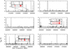 |
Fig. 3 NGC 7538–IRS1 spectra as observed with the IRAM-30 m telescope. Line assignment for CH3 CN and HNCO is shown in red. |
4.4 Temperature
The temperature diagram method (based on Eqs. (3) or (4) together with the observational line parameters) allows us to derive the temperature at which the targeted molecules are emitting in the observed ISM region. Figures 5–7 show the temperature diagrams derived from the analysis for the CH3CN, HNCO, and HCOOCH3 line emission, respectively. The resulting temperatures, T, are (350±31) K for CH3CN, (349±77) K for HNCO, and (182±44) K for HCOOCH3. The derived temperatures are consistent, for HNCO and HCOOCH3, with the previous study of this source by Bisschop et al. (2007).
4.5 Column densities
The total column density, N, of a molecule can be obtained from Eqs. (3) or (4) using the partition function, Q(T), at the derived excitation temperature. In this paper, we aim to quantify the impact of the partition function on the derived total column density. In that context, we used different approximations of the partition function to derive the total beam-averaged11 column density for CH3CN, HNCO, and HCOOCH3. The results are given in Table 7 for the rotational-vibrational(-torsional) partition functions obtained in the present study (third and seventh columns of Table 2 for CH3CN and HNCO, respectively, and third column of Table 6 for HCOOCH3) and for the approximations reported in the JPL or CDMS catalogs. In addition, we compared a linear and a nonlinear interpolation carried out at the temperature of NGC 7538 survey. The more reliable estimate of the total column density is the one that is calculated with the partition functions computed in the present study and given in the Col. 8 of Table 7. It can be noted that the nonlinear interpolation of the partition function given in the present study (see Appendix B) provides the same result for the total column densities. The relative difference between the different methods (see Table 7) is discussed in Sect. 5.
5 Discussion: implications of the partition function on the ISM molecular column densities
In this section we show how the use of different approximations for the rovibrational partition function together with some interpolation and/or extrapolation procedures affects estimations of the interstellar molecular column density. In that context, Table 7 gives the ISM column densities for CH3CN, HNCO, and HCOOCH3 derived from two different approximations of the respective partition functions. The calculations make use of the excitation temperatures given in Sect. 4.4 along with the partition functions obtained in the present study (see Table 2 for CH3CN and HNCO and Table 6 for HCOOCH3) and in the CDMS and/or JPL catalogs.
In our work, the rovibrational partition function is computed as the product of the rotational contribution, given as a direct sum, the harmonic approximation of the vibrational partition function, and, in the case of methyl formate, the torsional contribution computed as a direct sum (see above sections). To estimate the total column density in the survey NGC 7538, the partition function in the present study has been calculated at the specific temperatures of 350.33 K for CH3CN, 349.23 K for HNCO, and 182.46 K for HCOOCH3 (see Tables D.1–D.3, available at the CDS), obtained from Figs. 5–7, respectively. Moreover, because in general the partition functions are reported at typically 150, 225, 300, and 500 K in Table 7 we also show the results obtained after interpolating (linear or nonlinear) their values at the excited temperatures of the molecular species. The nonlinear interpolation of the partition function in the present study provides almost the same result as the one computed.
For isocyanic acid, HNCO, we also indicate in Table 2 the value of the partition function from the CDMS catalog (Endres et al. 2016), which provides the rotational contribution for the partition function; the vibrational contribution is unfortunately missing. For methyl cyanide, CH3CN, the CDMS catalog provides the rovibrational contribution for the partition function but only the lowest frequencies of the vibrational fundamental modes up to 1200 cm−1 are taken into account. Finally, for methyl formate, HCOOCH3, the JPL catalog provides a value for the rotational and torsional contributions of the partition function but only considering the two lowest torsional states vt = 0 and 1.
It is notable that the difference between our calculated partition function values and that from the databases are rather large, especially for high temperatures (i.e., ≥200–300 K; see Table 2 for CH3CN and HNCO and Fig. 1 for HCOOCH3). The resulting differences for the derived ISM molecular column densities are of the same order, from 9% up to about 40%, as shown in Table 7. In addition, a salient point of Table 7 is that the relative differences between the column densities estimated using our partition function and that of the CDMS/JPL database are less important in the case of a nonlinear interpolation approximation than in the case of a linear one (9, 21, and 35 vs. 18, 30, and 43% for CH3CN, HNCO, and HCOOCH3, respectively), reflecting the importance of the contribution of the vibrational modes. This trend is observed for all three targeted O-bearing and N-bearing molecules (see Table 7). Incidentally, it is important to note that for molecules with low vibrational energy modes and large amplitude motions (large amplitude motions give rise to low-lying torsional energy modes) the effect of using a nonconvergent partition function is also quite drastic.
The importance of undertaking a convergence study of the partition function in the characteristic temperature range of ISM was highlighted for the first time in 2014 when methyl formate (HCOOCH3) was identified in Orion-KL from the ALMA Science Verification Observations (Favre et al. 2014). In that study, the methyl formate column density was derived and the values were higher by a factor of between two and five with respect to previous reported values (Favre et al. 2011). Such a discrepancy is almost of the same order of magnitude as the observational uncertainties resulting from the instruments, the data calibration, and analysis. Nonetheless, the ISM molecular abundances are used to constrain the astrochemical models, which aim to investigate their formation pathways. It is therefore crucial to involve a converged partition function and to test the adequacy of the various approximations made in the partition function to derive more accurate abundances, especially in the case of isotopolog species. Isotopic ratios, obtained computing the relative abundance between two isotopic molecular species, are valuable for understanding the chemical evolution of interstellar material together with the impact of interstellar gas-phase chemistry processes that may occur during their formation (e.g., see Charnley et al. 2004; Wirström et al. 2011; Favre et al. 2014). Therefore, the approximation order of the partition function and its level of convergence carried out to estimate isotopic ISM abundance ratios is relatively important and must be consistent for all the isotopologs. An incorrect partition function, or the use of different approximations for the partition functions between the isotopologs of a same molecular species, will result in incorrect isotopic ratios and therefore erroneous astronomical conclusions (e.g., see Favre et al. 2014). A comprehensive convergence study of the molecular partition function in the temperature range of ISM is therefore a necessity.
Finally, we emphasize that the vibrational partition function contributions used in our present study (see Tables 2 and 6) are still incomplete because we use the harmonic approximation even though this could represent a good approximation, as was mentioned in Sect. 3.2 when considering H2 S as an example. This deficiency could be overcome either by implementing the anharmonicity of the vibrational modes in the equation forthe vibrational partition function or by using its direct sum expression for the potentially populated vibrational energy term values in the ISM temperatures. At the present time, there is unfortunately no vibrational partition function analyticalequation involving the anharmonicities, nor are there often complete vibrational analyses for the most relevant astrophysical molecules, even though these would significantly benefit the partition function calculation. Indeed, the anharmonicity usually decreases the vibrational term values with respect to the harmonic values by increasing the exponential terms of thedirect sum of the vibrational partition functions, in comparison with the harmonic approximation. As a consequence, the molecular column densities could generally be even slightly higher if the anharmonicity were taken into account (Skouteris et al. 2016).
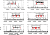 |
Fig. 4 NGC 7538–IRS1 spectra as observed with the IRAM-30 m telescope. Line assignment for HCOOCH3 is shown in red. |
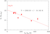 |
Fig. 5 CH3CN temperaturediagram in direction of NGC 7538–IRS1. Red dots indicate detected and partially detected lines. Error bars (3σ) only reflect the uncertainties in the Gaussian fit of the lines. |
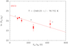 |
Fig. 6 HNCO temperature diagram in direction of NGC 7538–IRS1. Red dots indicate detected and partially detected lines, while dark triangles mark blended lines. Error bars (3σ) only reflect the uncertainties in the Gaussian fit of the lines. |
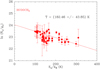 |
Fig. 7 HCOOCH3 temperaturediagram in direction of NGC 7538–IRS1. Red dots indicate detected and partially detected lines. Error bars (3σ) only reflect the uncertainties in the Gaussian fit of the lines. |
6 Conclusions
In the present study we investigate the impact of different approximations of the partition function together with some interpolation and/or extrapolation procedures on estimations of the interstellar molecular column density. For that purpose, we used astronomical observations of N- and O-bearing molecules with different symmetries. Our analysis shows that different methods can lead to a relative difference of up to 43%.
Our analysis has shown that considerable errors in the determination of the molecular column density can be overcome considering the following items.
- 1.
An appropriate convergence study of the partition function should be carried out in the temperature range of interest for the astronomical system under study in order to test the quality of the various approximations made while computing the partition function.
- 2.
The value of gns used in the calculation of Q should be checked before substituting it in the intensity equation.
- 3.
It could be beneficial to use precise interpolation and extrapolation approaches, that is, nonlinear fitting, for providing a rotational-vibrational(-torsional) partition function as a function of the temperature when the molecular column density is determined from the temperature diagram. Indeed, as shown in our study, a linear interpolation overestimates the partition function which leads to overestimation of the resulting molecular column densities.
It is important to emphasize that for computing a complete partition function, comprehensive information of the rotational, vibrational, and torsional (if appropriate) energy levels according to the excited temperature of the survey is necessary. In addition, the more complete the data set, the better the accuracy obtained for the partition function. Nevertheless, because of the lack of available spectroscopic data in the literature, one could take advantage of the present study to complete the partition functions of the molecules which could be incompletely converged for high-temperature ISM sources. It should be noted that in spite of the unfavorable estimate of the partition function uncertainties considering large uncertainties for the rotational-vibrational-torsional data, their relative values for the targeted molecules are small concerning the considered convergence limit smaller than 1%.
An extension of our work to other molecular species and surveys will be carried out in the near future, for example for propyne (CH3CCH), for which the present partition function only considers the vibrational states up to 700 cm−1 (Müller et al. 2002), or acetone (CH3C(O)CH3), and acetamide (CH3C(O)NH2), for which only the lowest torsional states are taken into account. This new study will allow us to verify if the partition functions converge in the temperature range of the surveys under study. In addition, these can be tabulated with polynomial coefficients to obtain an appropriate interpolation or extrapolation at the temperature of the survey. This extension will be particularly useful for surveys of sources with temperatures higher than 300 K which can be targeted in the future and in addition this could be relevant to future observations in the infrared, for example by the James Webb Space Telescope (JWST), SOFIA, the Space Infrared Telescope for Cosmology and Astrophysics (SPICA), and the Origins Space Telescope (OST).
Column density estimates of CH3CN, HNCO, and HCOOCH3 in NGC 7538 survey according to the partition function computed in the present study (rovibrational partition functions are computed as the product of the rotational contribution, given as a direct sum, the harmonic approximation of the vibrational partition function, and, for methyl formate, the torsional partition sum) and in the CDMS and JPL databases.
Acknowledgements
This work is partly supported by CMST COST Action CM1401 Our Astro-Chemical History and CMST COST Action CM1405 MOLIM. The work of C.F. is supported by the French National Research Agency in the framework of the Investissements d’Avenir program (ANR-15-IDEX-02), through the funding of the “Origin of Life” project of the Université Grenoble-Alpes. C.C. and C.F. acknowledge funding from the European Research Council (ERC) under the European Union’s Horizon 2020 research and innovation programme, for the Project “The Dawn of Organic Chemistry” (DOC), grant agreement No 741002. I.K. would like to thank the French programme of Chimie Interstellaire PCMI. C.F. and D.F. acknowledge support from the Italian Ministry of Education, Universities and Research, project SIR (RBSI14ZRHR). E.A.B. acknowledges support from NSF (AST-1514670) and NASA (NNX16AB48G). M.C. acknowledges the financial support from FIS2014-53448-C2-2-P (MINECO, Spain), from the Centro de Estudios Avanzados de Física, Matemáticas y Computación (CEAFMC) of the University of Huelva and from the Consejeríade Conocimiento, Investigación y Universidad, Junta de Andalucía and European Regional Development Fund (ERDF), ref. SOMM17/6105/UGR. The authors acknowledge the referee for his/her valuable comments.
Appendix A Nuclear spin statistics
In this appendix we discuss the different nuclear spin statistical weights used in the literature for isocyanic acid, methyl cyanide, and methyl formate.
A.1 Isocyanic acid (HNCO)
Isocyanic acid has a molecular symmetry  and therefore thenuclear spin statistical weight results in gns = 6 for both the A′ and A′′ states according to Bunker & Jensen (1989). In fact, gns has the same value for both symmetries, and therefore can be canceled out by the factor Q∕gu (see Eqs. (3) and (4)). As a result, we can assume that gns equals 6∕6 = 1. Consequently, in Tables 1 and 2, the gns value for isocyanic acid is givenequal to 1, such as in the CDMS catalog. The JPL partition function is however given with a reduced value of gns = 312. Thus, JPL and CDMS partition functions are different by a factor of three.
A.2 Methyl cyanide (CH3CN)
The main isotopolog of methyl cyanide (12 CH C14N) is a molecular species with symmetry
  . The nuclear spin statistical weight of each rovibrational state (symmetries A1, A2 and E) is gns = 12 (Bunker & Jensen 1989). As for HNCO (see Sects. 3.4 and 3.6.1), the nuclear spin statistical weight in Eqs. (3) and (4) can be canceled out since it appears in the left and in the right side of the equations.
Nevertheless, different normalized values of gns can be computed according to the author. In Table A.1, some of the nuclear spin degeneracy values computed in the literature (Bunker & Jensen 1989; Mangum & Shirley 2015; Rinsland et al. 2008; Blake et al. 1987; Turner 1991) are provided. The difference between all those values arises from the normalization factor (see Table A.1) used in the nuclear spin weight equation and its calculation is beyond the topic of this paper. Therefore, it is important to know the precise values of gns considered to compute the partition function (Eq. (5)), because the same values of gns should also be substituted into the gu factor (Eq. (2)) in the intensity expression (Eqs. (3) or (4)). Indeed, if the partition function of Eq. (5) is taken from a given reference and the nuclear spin weights from another and their values are different, this could give rise to erroneous astrochemical conclusions.
For instance, the rotational partition function calculated as a direct sum is Qrot(direct sum) ≈ 7588.7 at T = 300 K assuming gns = 1 (see Table 3) whereas the one published by the JPL and CDMS catalogs is ≈ 10 118 (4∕3 Qrot(direct sum)) which also differs from the one calculated by Rinsland et al. (2008): ≈60 709 (8 Qrot(direct sum)). Although the rotational partition function of Rinsland et al. (2008) is six times greater than that given by the JPL and CDMS databases and eight times greater than that used in the present study, all three values for the partition function agree with each other, after observing that they only differ by the normalization factor, which results from the different way of computing the nuclear spin statistical weight.
A.3 Methyl formate (HCOOCH3)
The main isotopolog of methyl formate (H12COO12CH3) belongs to the molecular symmetry group  . The nuclear spin statistical weight gns for each rovibrational state (symmetries A1, A2 and E) is equal to 8 (Bunker & Jensen 1989). Because it has the same value for every symmetry species states, gns can be considered equal to 1 in the intensity (Eqs. (3) and (4)). Therefore, the partition function given in Tables 4 and 6 and plotted in Fig. 1 does not take into account the nuclear spin statistical weight.
Nuclear statistical weight gns values for all symmetries of methyl cyanide according to the reference.
As for isocyanic acid and methyl cyanide, the nuclear spin degeneracy depends on the definition used by the author. For example, according to Blake et al. (1987) and Turner (1991), a normalized gns value equal to 2 is considered for the nondegenerate A-type as well as for the doubly degenerate E-type species13, such as is considered in the JPL catalog.
Appendix B Comparison of partition functions from nonlinear polynomial expansions and direct sums
In this appendix we provide the polynomial coefficients of Eqs. (11) and (12) which are fitted to the rotational-vibrational (-torsional) partition function values computed in the present study for isocyanic acid (HNCO), methyl cyanide (CH3CN), and methyl formate (H12COO12CH3).
B.1 Isocyanic acid
The rovibrational partition function values of the present study given in Table 2 have been fitted to the polynomial expansions given in Eqs. (11) and (12). The parameter values of the two nonlinear fits are given in Table B.1. To check the agreement between the rovibrational partition function computed using direct sums with the values provided by the polynomial expansions, their relative differences are also provided in Table B.1. From Table B.1 we can see that the sixth-order logarithm polynomial log10Q(T) of Eq. (12) has better agreement in general with the direct sum results than the Q(T) expansion of Eq. (11), in particular at low temperatures from 2.725 to 37.5 K. Above 37.5 K the logarithm expansion remains in reasonable agreement with Qrv (Present work), although the polynomial expansion of Q(T) is better.
Therefore, according to the small relative differences, both polynomial expansions can be considered to interpolate the rovibrational partition function of isocyanic acid at any temperature from 2.725 to 500 K. Hence, according to the better agreement of the fitted polynomial expansion at higher temperatures with respect to the nonlinear fit of the logarithm polynomial expansion, we decided to use the former one to interpolate the partition function at the temperature of NGC 7538 survey and so estimating the molecular column density (see Sects. 4 and 5).
B.2 Methyl cyanide
As in Sect. 3.6.1, the rovibrational partition function values of the present study for CH3CN (see Table 2) have been fitted to the polynomial expansions given in Eqs. (11) and (12). The parameter values of both nonlinear fits and the relative differences of the fitted polynomial expansions with respect to the rovibrational partition function values computed in the present study are given in Table B.2. On the one hand, the sixth-order expansion of Eq. (11) presents a good agreement except for temperatures below 10 K. On the other hand, the logarithm polynomial of Eq. (12) in general give a reasonable agreement with Qrv (Present work). Therefore, the two expansions can be used to interpolate the rovibrational partition function of methyl cyanide at any temperaturefrom 10 to 500 K.
In the present study, we have used the logarithm polynomial expansion to interpolate the rovibrational partition function of methyl cyanide at the temperature of NGC 7538 survey (see Sects. 4 and 5) because it is better in general.
B.3 Methyl formate
The rotational-vibrational-torsional partition function values of methyl formate computed in this study (see Col. 3 of Table 6), has been fitted with the two nonlinear polynomial expansions (see Eqs. (11) and (12)). The parameter values of these two fits are given in Table B.3. Table B.3 also shows the relative differences between the values of the rotational-vibrational-torsional partition function computed in the present study using the direct sum and the values of the partition function fitted using polynomial values. This comparison aims to select which fitting formula is more appropriate depending on the temperature ranges. In the present study we have considered the two expansions, the polynomial (Eq. (11)) and the decimal logarithm polynomial (Eq. (12)), up to sixth-order. As shown in Table B.3, the sixth-order polynomial from Eq. (11) undergoes the highest deviations: 36.45, −1.88 and −6.11% at the lowest temperatures, T = 2.725, 5 and 9.375 K, respectively. On the contrary, the fit of a power expansion of log10Q from Eq. (12) undergoes deviations smaller than 0.8% for all the temperature range (i.e. from T = 2.725 K up to 500 K). However, for temperatures higher than 75 K, the sixth-order polynomial from Eq. (11) provides deviations of the rotational-vibrational-torsional partition function values which are smaller than the deviations presented by the logarithm power expansion of Eq. (12). Hence, we can conclude that, for methyl formate, the temperature polynomial expansion is more suitable to interpolate the rotational-vibrational-torsional partition function at any temperature above 75 K while the decimal logarithm log10(T) polynomial expansion seems more appropriate for interpolating the partition function from 75 K down to temperatures around 3 K.
Polynomial coefficients fitted to the rovibrational partition function values computed in the present study for isocyanic acid (HNCO).
Polynomial coefficients fitted to the rovibrational partition function values of the present study for methyl cyanide (CH3 CN).
Polynomial coefficients fitted to the rotational-vibrational-torsional partition function values of the present study for methyl formate (H12COO12CH3).
Appendix C Spectroscopic and observational line parameters
The spectroscopic and observational line parameters for the molecular species HNCO, CH3CN and HCOOCH3 are given here.
Spectroscopic and observational line parameters for HNCO.
Spectroscopic and observational line parameters for CH3CN.
Spectroscopic and observational line parameters for HCOOCH3.
References
- Anttila, R., Horneman, V.-M., Koivusaari, M., & Paso, R. 1993, J. Mol. Spectr., 57, 198 [NASA ADS] [CrossRef] [Google Scholar]
- Barton, E. J., Chiu, C., Golpayegani, S., et al. 2014, MNRAS, 442, 1821 [NASA ADS] [CrossRef] [Google Scholar]
- Bauder, A. 1979, J. Chem. Phys., 583, 31 [Google Scholar]
- Bisschop, S. E., Jørgensen, J. K., van Dishoeck, E. F., & de Wachter, E. B. M. 2007, A&A, 465, 913 [NASA ADS] [CrossRef] [EDP Sciences] [Google Scholar]
- Blake, G. A., Sutton, E. C., Masson, C. R., & Phillips, T. G. 1987, ApJ, 315, 621 [NASA ADS] [CrossRef] [Google Scholar]
- Boucher, D., Burie, J., Demaison, J., et al. 1977, J. Mol. Spectr., 64, 290 [NASA ADS] [CrossRef] [Google Scholar]
- Brown, R. D., Crofts, J. G., Gardner, F. F., et al. 1975, ApJ, 197, 29 [Google Scholar]
- Bunker, P. R., & Jensen, P. 1989, Molecular Symmetry and Spectroscopy (Ottawa: NRC Research Press) [Google Scholar]
- Carvajal, M., & Lemus, R. 2015, J. Phys. Chem. A, 119, 12823 [CrossRef] [Google Scholar]
- Carvajal, M., Willaert, F., Demaison, J., & Kleiner, I. 2007, J. Mol. Spectr., 246, 158 [NASA ADS] [CrossRef] [Google Scholar]
- Carvajal, M., Margulès, L., Tercero, B., et al. 2009, A&A, 500, 1109 [NASA ADS] [CrossRef] [EDP Sciences] [Google Scholar]
- Carvajal, M., Kleiner, I., & Demaison, J. 2010, ApJS, 190, 315 [NASA ADS] [CrossRef] [Google Scholar]
- Cazzoli, G., & Puzzarini, C. 2006, J. Mol. Spectr., 240, 153 [NASA ADS] [CrossRef] [Google Scholar]
- Cerezo, J., Bastida, A., Requena, A., & Zuñiga, J. 2014, J. Quant. Spectr. Rad. Transf., 147, 233 [NASA ADS] [CrossRef] [Google Scholar]
- Chao, J., Hall, K. R., Marsh, K. N., & Wilhoit, R. C. 1986, J. Phys. Chem. Ref. Data, 15, 1369 [NASA ADS] [CrossRef] [Google Scholar]
- Charnley, S. B., Ehrenfreund, P., & Millar, T. J. 2004, MNRAS, 347, 157 [NASA ADS] [CrossRef] [Google Scholar]
- Codella, C., Ceccarelli, C., Cabrit, S., et al. 2016, A&A, 586, L3 [CrossRef] [EDP Sciences] [Google Scholar]
- Curl, R. F. 1959, J. Chem. Phys., 30, 1529 [NASA ADS] [CrossRef] [Google Scholar]
- Demaison, J., Boucher, D., Dubrulle, A., & Eijck, B. P. V. 1983, J. Mol. Spectr., 102, 260 [NASA ADS] [CrossRef] [Google Scholar]
- Duan, C., Carvajal, M., Yu, S., et al. 2015, A&A, 576, A39 [NASA ADS] [CrossRef] [EDP Sciences] [Google Scholar]
- East, A. L. L., Johnson, C. S., & Allen, W. D. 1993, J. Chem. Phys., 98, 1299 [NASA ADS] [CrossRef] [Google Scholar]
- Elkeurti, M., Coudert, L. H., Medvedev, I. R., et al. 2010, J. Mol. Spectr., 263, 145 [NASA ADS] [CrossRef] [Google Scholar]
- Endres, C. P., Schlemmer, S., Schilke, P., Stutzki, J., & Müller, H. S. P. 2016, J. Mol. Spectr., 327, 95 [NASA ADS] [CrossRef] [Google Scholar]
- Favre, C., Despois, D., Brouillet, N., et al. 2011, A&A, 532, A32 [NASA ADS] [CrossRef] [EDP Sciences] [Google Scholar]
- Favre, C., Carvajal, M., Field, D., et al. 2014, ApJS, 215, 25 [NASA ADS] [CrossRef] [Google Scholar]
- Fischer, J., & Gamache, R. R. 2002, J. Quant. Spectr. Rad. Transf., 74, 263 [NASA ADS] [CrossRef] [Google Scholar]
- Fischer, J., Gamache, R. R., Goldman, A., Rothman, L., & Perrin, A. 2003, J. Quant. Spectr. Rad. Transf., 82, 401 [Google Scholar]
- Furtenbacher, T., Szabó, I., Császár, A., et al. 2016a, ApJS, 224, 44 [NASA ADS] [CrossRef] [Google Scholar]
- Furtenbacher, T., Szidarovszky, T., Hrubý, J., et al. 2016b, J. Phys. Chem. Ref. Data, 45, 043104 [NASA ADS] [CrossRef] [Google Scholar]
- Gadhi, J., Lahrouni, A., & Legrand, J. 1995, J. Chem. Phys., 92, 1984 [Google Scholar]
- Goldsmith, P. F., & Langer, W. D. 1999, ApJ, 517, 209 [NASA ADS] [CrossRef] [Google Scholar]
- Gamache, R., Roller, C., Lopes, E., et al. 2017, J. Quant. Spectr. Rad. Transf., 203, 70 [NASA ADS] [CrossRef] [Google Scholar]
- Gordon, I., Rothman, L., Hill, C., et al. 2017, J. Quant. Spectr. Rad. Transf., 203, 3 [Google Scholar]
- Groner, P., Winnewisser, M., Medvedev, I. R., & et al. 2007, ApJS, 169, 28 [NASA ADS] [CrossRef] [Google Scholar]
- Haykal, I., Carvajal, M., Tercero, B., et al. 2014, A&A, 568, A58 [NASA ADS] [CrossRef] [EDP Sciences] [Google Scholar]
- Herbst, E., & van Dishoeck, E. F. 2009, ARA&A, 47, 427 [NASA ADS] [CrossRef] [Google Scholar]
- Herzberg, G. 1991, Spectra and Molecular Structure: II. Infrared and Raman Spectra of Polyatomic Molecules (Malabar, FL: Krieger Pub. Co.) [Google Scholar]
- Hocking, W. H., Gerry, M. C. L., & Winnewisser, G. 1975, Can. J. Phys., 53, 1869 [NASA ADS] [CrossRef] [Google Scholar]
- Ilyushin, V., Kryvda, A., & Alekseev, E. 2009, J. Mol. Spectr., 255, 32 [NASA ADS] [CrossRef] [Google Scholar]
- Irwin, A. W. 1981, ApJS, 45, 621 [NASA ADS] [CrossRef] [Google Scholar]
- Karakawa, Y., Oka, K., Odashima, H., Takagi, K., & Tsunekawa, S. 2001, J. Mol. Spectr., 210, 196 [NASA ADS] [CrossRef] [Google Scholar]
- Kleiner, I. 2010, J. Mol. Spectr., 260, 1 [NASA ADS] [CrossRef] [Google Scholar]
- Kleiner, I., Hougen, J. T., Grabow, J.-U., et al. 1996, J. Mol. Spectr., 179, 41 [NASA ADS] [CrossRef] [Google Scholar]
- Kleiner, I., Georges, R., Hepp, M., & Herman, M. 1999, J. Mol. Spectr., 193, 228 [NASA ADS] [CrossRef] [Google Scholar]
- Kleiner, I., Moazzen-Ahmadi, N., McKellar, A. R. W., et al. 2008, J. Mol. Spectr., 252, 214 [NASA ADS] [CrossRef] [Google Scholar]
- Kobayashi, K., Takamura, K., Sakai, Y., et al. 2013, ApJS, 205, 9 [NASA ADS] [CrossRef] [Google Scholar]
- Kobayashi, K., Kuwahara, T., Tachi, H., et al. 2018, J. Mol. Spectr., 343, 50 [NASA ADS] [CrossRef] [Google Scholar]
- Kukolich, S. G. 1982, J. Chem. Phys., 76, 97 [NASA ADS] [CrossRef] [Google Scholar]
- Kukolich, S. G., Nelson, A. C., & Yamanashi, B. S. 1971, J. Am. Chem. Soc., 93, 6769 [CrossRef] [Google Scholar]
- Kukolich, S. G., Ruben, D. J., Wang, J. H. S., & Williams, J. R. 1973, J. Chem. Phys., 58, 3155 [NASA ADS] [CrossRef] [Google Scholar]
- Lapinov, A. V., Golubiatnikov, G. Y., Markov, V. N., & Guarnieri, A. 2007, Astron. Lett., 33, 121 [NASA ADS] [CrossRef] [Google Scholar]
- Loren, R., & Mundy, L. G. 1984, ApJ, 286, 232 [NASA ADS] [CrossRef] [Google Scholar]
- Lovas, F. J. 2004, J. Phys. Chem. Ref. Data, 33, 177 [NASA ADS] [CrossRef] [Google Scholar]
- Maeda, A., Medvedev, I. R., DeLucia, F. C., & Herbst, E. 2008a, J. Mol. Spectr., 251, 293 [NASA ADS] [CrossRef] [Google Scholar]
- Maeda, A., Medvedev, I. R., DeLucia, F. C., Herbst, E., & Groner, P. 2008b, ApJS, 175, 138 [NASA ADS] [CrossRef] [Google Scholar]
- Mangum, J. G., & Shirley, Y. L. 2015, PASP, 127, 266 [NASA ADS] [CrossRef] [Google Scholar]
- Margulès, L., Huet, T. R., Demaison, J., et al. 2010, ApJ, 714, 1120 [NASA ADS] [CrossRef] [Google Scholar]
- Margulès, L., Motiyenko, R. A., Ilyushin, V. V., & Guillemin, J. C. 2015, A&A, 579, A46 [NASA ADS] [CrossRef] [EDP Sciences] [Google Scholar]
- Martín, S., Martín-Pintado, J., & Mauersberger, R. 2006, A&A, 450, L13 [NASA ADS] [CrossRef] [EDP Sciences] [Google Scholar]
- McDowell, R. S. 1990, J. Chem. Phys., 93, 2801 [NASA ADS] [CrossRef] [Google Scholar]
- Müller, H. S. P., Pracna, P., & Horneman, V.-M. 2002, J. Mol. Spectr., 216, 397 [NASA ADS] [CrossRef] [Google Scholar]
- Müller, H. S. P., Schlöder, F., Stutzki, J., & Winnewisser, G. 2005, J. Mol. Struct., 742, 215 [NASA ADS] [CrossRef] [Google Scholar]
- Müller, H. S. P., Drouin, B. J., & Pearson, J. C. 2009, A&A, 506, 1487 [NASA ADS] [CrossRef] [EDP Sciences] [Google Scholar]
- Müller, H. S. P., Brown, L. R., Drouin, B. J., et al. 2015, J. Mol. Spectr., 312, 22 [NASA ADS] [CrossRef] [Google Scholar]
- Niedenhoff, M., Yamada, K. M. T., Belov, S. P., & Winnewisser, G. 1995, J. Mol. Spectr., 174, 151 [NASA ADS] [CrossRef] [Google Scholar]
- Odashima, H., Ogata, K., Takagi, K., & Tsunekawa, S. 2003, Molecules, 8, 139 [CrossRef] [Google Scholar]
- Oesterling, L. C., Albert, S., DeLucia, F. C., & Blake, G. A. 1999, ApJ, 521, 255 [NASA ADS] [CrossRef] [Google Scholar]
- Ogata, K., Odashima, H., Takagi, K., & Tsunekawa, S. 2004, J. Mol. Spectr., 225, 14 [NASA ADS] [CrossRef] [Google Scholar]
- Pearson, J. C., Daly, A. M., & Lees, R. M. 2015, J. Mol. Spectr., 318, 70 [NASA ADS] [CrossRef] [Google Scholar]
- Pickett, H. M. 1991, J. Mol. Spectr., 148, 371 [NASA ADS] [CrossRef] [Google Scholar]
- Pickett, H. M., Poynter, R. L., Cohen, E. A., et al. 1998, J. Quant. Spectr. Rad. Transf., 60, 883 [NASA ADS] [CrossRef] [Google Scholar]
- Plummer, G. M., Blake, G. A., Herbst, E., & DeLucia, F. C. 1984, ApJS, 55, 633 [NASA ADS] [CrossRef] [Google Scholar]
- Plummer, G. M., Herbst, E., DeLucia, F. C., & Blake, G. A. 1986, ApJS, 60, 949 [NASA ADS] [CrossRef] [Google Scholar]
- Remijan, A. J., Markwick-Kemper, A., & the ALMA Working Group on Spectral Line Frequencies. 2007, BAAS, 38, 963 [NASA ADS] [Google Scholar]
- Rinsland, C. P., Devi, V. M., Benner, D. C., et al. 2008, J. Quant. Spectr. Rad. Transf., 109, 974 [NASA ADS] [CrossRef] [Google Scholar]
- Senent, M. L., Villa, M., Meléndez, F. J., & Domínguez-Gómez, R. 2005, ApJ, 627, 567 [NASA ADS] [CrossRef] [Google Scholar]
- Shaw, A. M. 2006, Astrochemistry: From Astronomy to Astrobiology (Chichester: John Wiley & Sons, Ltd.) [Google Scholar]
- Skouteris, D., Calderini, D., & Barone, V. 2016, J. Chem. Theory Comput., 12, 1011 [CrossRef] [Google Scholar]
- Slocum, D. M., Xu, L.-H., Giles, R. H., & Goyette, T. M. 2015, J. Mol. Spectr., 318, 12 [NASA ADS] [CrossRef] [Google Scholar]
- Smirnov, I. A., Alekseev, E. A., Ilyushin, V. V., et al. 2014, J. Mol. Spectr., 295, 44 [NASA ADS] [CrossRef] [Google Scholar]
- Takano, S., Sakai, Y., Kakimoto, S., Sasaki, M., & Kobayashi, K. 2012, PASJ, 64, 89 [NASA ADS] [Google Scholar]
- Tercero, B., Margulès, L., Carvajal, M., et al. 2012, A&A, 538, A119 [NASA ADS] [CrossRef] [EDP Sciences] [Google Scholar]
- Tudorie, M., Ilyushin, V., Auwera, J. V., et al. 2012, J. Chem. Phys., 137, 064304 [NASA ADS] [CrossRef] [Google Scholar]
- Turner, B. E. 1991, ApJS, 76, 617 [NASA ADS] [CrossRef] [Google Scholar]
- Voronkov, M. A., Austin, M. C., & Sobolev, A. M. 2002, A&A, 387, 310 [NASA ADS] [CrossRef] [EDP Sciences] [Google Scholar]
- Wang, S., Bergin, E. A., Crockett, N. R., et al. 2011, A&A, 527, A95 [NASA ADS] [CrossRef] [EDP Sciences] [Google Scholar]
- Willaert, F., Møllendal, H., Alekseev, E., et al. 2006, J. Mol. Struct., 795, 4 [NASA ADS] [CrossRef] [Google Scholar]
- Wirström, E. S., Geppert, W. D., Hjalmarson, A., et al. 2011, A&A, 533, A24 [NASA ADS] [CrossRef] [EDP Sciences] [Google Scholar]
- Xu, L.-H., Fisher, J., Lees, R. M., et al. 2008, J. Mol. Spectr., 251, 305 [NASA ADS] [CrossRef] [Google Scholar]
- Xu, L.-H., Lees, R. M., Hao, Y., et al. 2014, J. Mol. Spectr., 303, 1 [NASA ADS] [CrossRef] [Google Scholar]
- Zaleski, D. P., Duan, C., Carvajal, M., Kleiner, I., & Prozument, K. 2017, J. Mol. Spectr., 342, 17 [NASA ADS] [CrossRef] [Google Scholar]
- Zheng, J., Mielke, S. L., Clarkson, K. L., & Truhlar, D. G. 2012, Comput. Phys. Commun., 183, 1803 [NASA ADS] [CrossRef] [Google Scholar]
This database also collects data from other catalogues, https://www.cv.nrao.edu/php/splat/
Also referred to as Total Internal Partition Sums (TIPS; Fischer & Gamache 2002) and ideal-gas internal partition function (Furtenbacher et al. 2016b).
The complete internal wavefunction is the eigenfunction of the complete Hamiltonian for the internal dynamics of the molecule, which includes the rovibronic, electron spin, and nuclear spin degrees of freedom (Bunker & Jensen 1989).
In this study, we assume a source equal to that of the beam.
The values of gns can be obtained by different procedures (e.g., see, Bunker & Jensen 1989; Mangum & Shirley 2015) and therefore can have different values.
Blake et al. (1987) and Turner (1991) consider that gK = 1 and gI = 2 for the nondegenerate A-type and gK = 2 and gI = 1 for the doubly degenerate E-type species so, according to Eq. (10), gns = gI gK = 2.
All Tables
Vibrational and rotational-vibrational partition function for methyl cyanide (CH3 CN) and isocyanicacid (HNCO).
Torsional(a) and vibrational contributions of the partition function for methyl formate (HCOOCH3).
Rotational-torsional-vibrational partition function (a) for main isotopolog of methyl formate (H12COO12CH3).
Column density estimates of CH3CN, HNCO, and HCOOCH3 in NGC 7538 survey according to the partition function computed in the present study (rovibrational partition functions are computed as the product of the rotational contribution, given as a direct sum, the harmonic approximation of the vibrational partition function, and, for methyl formate, the torsional partition sum) and in the CDMS and JPL databases.
Nuclear statistical weight gns values for all symmetries of methyl cyanide according to the reference.
Polynomial coefficients fitted to the rovibrational partition function values computed in the present study for isocyanic acid (HNCO).
Polynomial coefficients fitted to the rovibrational partition function values of the present study for methyl cyanide (CH3 CN).
Polynomial coefficients fitted to the rotational-vibrational-torsional partition function values of the present study for methyl formate (H12COO12CH3).
All Figures
|
Fig. 1 Convergence study of the partition function for methyl formate. Comparison of the partition function values computed in the present study (full red circles) and JPL database (full green squares). The linear interpolation of the partition function computed in the present study is given as red dashed lines while the nonlinear sixth-order polynomial fit is given as a blue line. From JPL, the linear interpolation and the nonlinear fit (green line) are apparently overlapped. The differences between the two partition functions are due to the fact that the JPL partition function does not include the vibrational contribution and does take into account the torsional contribution from Eq. (9) only up to vt = 0 and 1, whereas we are including torsional levels up to vt = 10 as well as the vibrational contribution. |
| In the text | |
|
Fig. 2 Logarithm of Q in base 10 is provided according to calculation of the present study (full red circles). The nonlinear sixth-order decimal logarithm polynomial curve fitting (blue line) is provided up to T = 800 K. This result is compared with the extrapolated values obtained using the partition function at T = 300 K as benchmark (brown line) (see Eq. (13)). In addition, it has been included the extrapolated values computed with Eq. (13) but using T = 500 K as benchmark (green line). |
| In the text | |
|
Fig. 3 NGC 7538–IRS1 spectra as observed with the IRAM-30 m telescope. Line assignment for CH3 CN and HNCO is shown in red. |
| In the text | |
|
Fig. 4 NGC 7538–IRS1 spectra as observed with the IRAM-30 m telescope. Line assignment for HCOOCH3 is shown in red. |
| In the text | |
|
Fig. 5 CH3CN temperaturediagram in direction of NGC 7538–IRS1. Red dots indicate detected and partially detected lines. Error bars (3σ) only reflect the uncertainties in the Gaussian fit of the lines. |
| In the text | |
|
Fig. 6 HNCO temperature diagram in direction of NGC 7538–IRS1. Red dots indicate detected and partially detected lines, while dark triangles mark blended lines. Error bars (3σ) only reflect the uncertainties in the Gaussian fit of the lines. |
| In the text | |
|
Fig. 7 HCOOCH3 temperaturediagram in direction of NGC 7538–IRS1. Red dots indicate detected and partially detected lines. Error bars (3σ) only reflect the uncertainties in the Gaussian fit of the lines. |
| In the text | |
Current usage metrics show cumulative count of Article Views (full-text article views including HTML views, PDF and ePub downloads, according to the available data) and Abstracts Views on Vision4Press platform.
Data correspond to usage on the plateform after 2015. The current usage metrics is available 48-96 hours after online publication and is updated daily on week days.
Initial download of the metrics may take a while.