| Issue |
A&A
Volume 593, September 2016
|
|
|---|---|---|
| Article Number | L13 | |
| Number of page(s) | 6 | |
| Section | Letters | |
| DOI | https://doi.org/10.1051/0004-6361/201628968 | |
| Published online | 22 September 2016 | |
Sub-0.1′′ optical imaging of the Z CMa jets with SPHERE/ZIMPOL
1 INAF–Osservatorio Astronomico di Roma, via Frascati 33, 00078 Monte Porzio Catone, Italy
e-mail: This email address is being protected from spambots. You need JavaScript enabled to view it.
2 INAF–Osservatorio Astrofisico di Arcetri, Largo E. Fermi 5, 50125 Firenze, Italy
3 Laboratoire Lagrange (UMR 7293), UNSA, CNRS, Observatoire de la Côte d’Azur, Bd de l’Observatoire, 06304 Nice Cedex 4, France
4 INAF–Osservatorio Astronomico di Padova, Vicolo dell’Osservatorio 5, 35122 Padova, Italy
5 Dipartimento di Fisica e Astronomia, Università degli Studi di Padova, Vicolo dell’Osservatorio 3, 35122 Padova, Italy
6 Dipartimento di Informatica, Bioingegneria, Robotica e Ingegneria dei Sistemi (DIBRIS), Università di Genova, via Dodecaneso 35, 16145 Genova, Italy
7 Institute for Astronomy, ETH Zürich, Wolfgang-Pauli-Strasse 27, 8093 Zürich, Switzerland
8 Université Grenoble Alpes, IPAG, 38000 Grenoble, France
9 CNRS, IPAG, 38000 Grenoble, France
10 Université Lyon, Université Lyon1, Ens de Lyon, CNRS, CRAL UMR 5574, 69230 Saint-Genis-Laval, France
11 Aix-Marseille Université, CNRS, LAM – Laboratoire d’Astrophysique de Marseille, UMR 7326, 13388 Marseille, France
Received: 19 May 2016
Accepted: 11 August 2016
Abstract
Context. Crucial information on the mass accretion-ejection connection in young stars can be obtained from high spatial resolution images of jets in sources with known recurrent accretion outbursts.
Aims. Using the VLT/SPHERE ZIMPOL instrument, we observed the young binary Z CMa that is composed of a Herbig Be star and a FUor object, both driving a jet. We aim to analyse the structure of the two jets, their relation with the properties of the driving sources, and their connection with previous accretion events observed in this target.
Methods. We obtained optical images in the Hα and [O i] 6300 Å lines at the unprecedented angular resolution of ~0.03 arcsec, on which we have performed both continuum subtraction and deconvolution, thereby deriving results that are consistent with each other.
Results. Our images reveal extended emission from both sources: a fairly compact and poorly collimated emission SW of the Herbig component and an extended collimated and precessing jet from the FUor component. The compact emission from the Herbig star is compatible with a wide-angle wind and is possibly connected to the recent outburst events shown by this component. The FUor jet is traced down to 70 mas (80 AU) from the source and is highly collimated with a width of 26−48 AU at distances 100−200 AU, which is similar to the width of jets from T Tauri stars. This strongly suggests that the same magneto-centrifugal jet-launching mechanism also operates in FUors. The observed jet wiggle can be modelled as originating from an orbital motion with a period of 4.2 yr around an unseen companion with mass between 0.48 and 1 M⊙. The jet mass loss rate Ṁjet was derived from the [O i] luminosity and comprises of between 1 × 10⁻⁸ and 1 × 10⁻⁶M⊙ yr-1. This is the first direct Ṁjet measurement from a jet in a FUor. If we assume previous mass accretion rate estimates obtained through modelling of the accretion disk, the derived range of Ṁjet would imply a very low mass-ejection efficiency (Ṁjet/Ṁacc≲ 0.02), which is lower than that typical of T Tauri stars.
Key words: stars: pre-main sequence / stars: variables: T Tauri, Herbig Ae/Be / stars: winds, outflows / stars: individual: Z CMa / techniques: high angular resolution / circumstellar matter
© ESO, 2016
1. Introduction
Star formation occurs through a mechanism that couples accretion from a disk and ejection of matter in the form of winds and collimated jets, which concur in removing angular momentum from the system. The accretion process is considered to be quasi-stationary, but time-variable accretion bursts caused by a quick rise of the mass accretion rate from the disk are sometimes observed. Studies of jets from sources that show episodic accretion events allow one to trace the past history of the accretion bursts, as one may expect to detect spatial structures within the jet that can be connected with particularly intense mass-ejection events. Fundamental insights come from the inner regions close to the source, where the jets are less contaminated by interactions with the ambient medium, so that their morphology can be tightly connected with variations of the ejection efficiency.
The Z CMa binary is a peculiar system that is suited to investigate the occurrence of mass ejection in young sources undergoing episodic accretion. This binary is composed of a Herbig Be star (the NW component), which shows EXor-like outbursts (Szeifert et al. 2010), and a second component (SE) that exhibits broad double-peaked optical absorption lines that are typical of a FU Ori object (Hartmann et al. 1989; Hartmann & Kenyon 1996). The two sources, located at a distance of 1150 pc (Herbst et al. 1978), are separated by 0.̋1 and only recently high angular resolution observations with adaptive optics (AO) systems and interferometers have allowed the separatele determination of the properties of the two sources (Bonnefoy et al. 2016; Hinkley et al. 2013). The Herbig star, which is responsible for the variability of the binary (Bonnefoy et al. 2016), has shown recurrent variations in the visual magnitude of 2−3 mag in the last ten years with recent major events recorded in 2008, 2011, and 2015 (see light curves in Canovas et al. 2012; Maehara & Ukita 2015). These variations have been imputed to both variable accretion and to changes of the extinction along the line of sight (Benisty et al. 2010; Szeifert et al. 2010).
An extended optical jet from Z CMa was originally detected by Poetzel et al. (1989). Recently, Whelan et al. (2010, hereafter W10) discovered that both sources drive their own jet, at slightly different position angles (PA): 245° (east of north) for the Herbig and 235° for the FU Ori. The jet from the NW source has a very high radial velocity reaching up to −600 km s-1 while the jet from the SE component has a velocity of ~−200/−300 km s-1. The large-scale optical jet observed by Poetzel et al. (1989) is usually associated with the Herbig component (e.g. Garcia et al. 1999; W10). Additional emission that is not collimated well is observed at intermediate velocities, which cannot however be unambiguously associated with one of the two components (W10). The analysis of these jets offers us the opportunity to obtain direct information on the mass loss and indirect information on the accretion rate. This is especially interesting in the case of the FUor component, since no direct mass loss measurements from jets are available for such objects. Wind mass loss rates as high as 10-5M⊙ yr-1were estimated on the prototype source FU Ori from line profiles (Croswell et al. 1987; Calvet et al. 1993). Accretion rates estimates for FUor objects are also very scarce and range from 10-4 to 10-6M⊙ yr-1 (Audard et al. 2014).
We present here VLT/SPHERE (Beuzit et al. 2008) high angular resolution optical observations of Z CMa in the [O i]6300 Å and Hα lines. The extreme AO performance of SPHERE allows us to have direct images of the Z CMa system at unprecedented high contrast and spatial resolution (~0.̋03).
2. Observations and data reduction
Observations of Z CMa in the Hα and [O i] lines were performed using the ZIMPOL instrument (Thalmann et al. 2008; Schmid et al. 2012) of SPHERE on the night of 31 March 2015. Simultaneous images of Z CMa in Hα and in the adjacent continuum were acquired with the two ZIMPOL cameras using the B_Ha (λc = 655.6 nm, Δλ = 5.5 nm) and Cnt_Ha (λc = 644.9 nm, Δλ = 4.1 nm) filters. Exposures were taken in field-stabilized mode using two different field rotation angles and swapping the filters in front of each camera to optimize artefact removal during the reduction. This resulted in 60 frames per filter (15 for each setup) for a total exposure time of 30 min. Images in the [O i] line with the OI_630 filter1 (λc = 629.5 nm, Δλ = 5.4 nm) were obtained in field-stabilized mode using two different field rotation angles for a total of 30 frames and an integration time of 30 min. Atmospheric conditions remained stable during observations (seeing ~0.̋8−1′′, τ0 ~ 2.5 ms).
The raw data were processed using the SPHERE-ZIMPOL IDL pipeline (version 1.1) developed at ETH Zürich, which performs bias, dark, flat-field correction, re-centring of the dithered frames, and allows for derotation, selection, subtraction, and average or median combination of the frames. The Cnt_Ha exposures were used to remove the continuum emission from the B_Ha and OI_630 filter images, so as to produce continuum-subtracted Hα and [O i] images in which the line-emitting structures around the components are evidenced. Details about the reduction procedure for the continuum subtraction are given in Appendix A. From the FWHM of the PSF of the two stars measured in the Cnt_Ha frames we estimate an effective angular resolution of ~30 mas for our images. The binary separation and position angle are analysed in Appendix B.
We also performed an alternative processing of the ZIMPOL images with the multi-component Richardson-Lucy (MC-RL) deconvolution method developed by La Camera et al. (2014), which is optimized for the reconstruction of high dynamical range images, such as those of jets from young stars (e.g. Antoniucci et al. 2014). The MC-RL method is able to separately reconstruct the star(s) and the underlying diffuse emission in the image. We extracted the PSF from the Cnt_Ha image via the blind deconvolution algorithm described in Prato et al. (2013, 2015) and employed to reconstruct both the [O i] and Hα images.
3. Results and discussion
The final continuum-subtracted [O i] and Hα images are shown in the upper part of Figs. 1a,b. We can recognise two major structures: an extended collimated jet from the FUor component and a more compact and poorly collimated emission SW of the Herbig star. These structures are especially evident in the [O i] image, which is much less affected by subtraction residuals than the Hα image. In our [O i] continuum-subtracted image we can trace the flows down to about ~90 mas from the sources (corresponding to ~105 AU). The morphology of both the FUor jet and the compact emission from the Herbig is thoroughly confirmed by the deconvolved images (lower part of Figs. 1a,b), which represent the diffuse emission in the image as reconstructed by the MC-RL algorithm. The [O i] deconvolved image shows details of the FUor jet even closer to driving source, down to ~70 mas (80 AU). The deconvolved Hα image provides evidence of the non-collimated emission SW of the Herbig star, which was not fully visible in the continuum-subtracted image owing to the large residuals.
3.1. Outflow from the Herbig Be star
The extended [O i] and Hα emission detected SW of the Herbig star is fairly compact and poorly collimated, suggesting an origin in a wide-angle wind more than in a jet. The flow has an extent of ~0.̋12, corresponding to ~140 AU, while the observed opening angle is ~ 55° with a median P.A. around 230°. In [Fe ii] KECK observations by W10, collimated emission travelling at velocities up to −600 km s-1 and with a PA ~ 245° is detected up to distances of 0.̋4 from the source, along with a more diffuse emission at lower velocities (100−200 km s-1). The wide-angle compact emission that we observe is likely connected to this diffuse emission, while the high-velocity collimated jet is not visible in our images. Although the Herbig jet is visible at high velocities in the [Fe ii] data reported by W10 (which are not flux calibrated), the flux contrast between the FUor and Herbig jet is indeed greater than a factor ~20 for velocities between −400 and −90 km s-1. This also agrees with the non-detection of the jet in the SINFONI data shown by W10. As we can estimate a mean signal-to-noise ratio of about 12 on the FUor jet, we conclude that we did not observe the collimated jet from the Herbig because of sensitivity limits.
Interferometric measurements of the Brγ line during the 2008 outburst (Benisty et al. 2010) suggested a bipolar (non fully spherical) wind from the star on mas scales, roughly aligned in the direction of the large-scale jet. As the Brγ emission disappeared outside the outburst phase, the authors concluded that the wind emission is connected to the event of increased mass accretion driving the outburst. To understand if the emission detected in our images is related to such bipolar wind, we evaluated whether the signal may be attributed to an ejection event from the recent Herbig star bursts, which occurred in January 2008 and February 2011 (Canovas et al. 2012), and more recently in January 2015 (see photometry from the Kamogata Wide-field Survey Maehara & Ukita 2015). Given the observed extent of the flow, we find that it should travel at a tangential velocity of 90, 170, and 2700 km s-1 to have been ejected from the 2008, 2011, or 2015 events, respectively. Ruling out the latter event, which implies an exceedingly large velocity, a connection with the 2008 and 2011 events is possible.
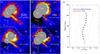 |
Fig. 1 a)Continuum-subtracted (top) and deconvolved (bottom) [O i] images of the Z CMa system. The deconvolved image shows only the diffuse emission as reconstructed by the MC-RL algorithm. The centroids of the two stars and the position of the main knots of the FUor jet are indicated. Areas heavily corrupted by artefacts around the star centroids have been masked. b) Same for the Hα observations. c) Fitted transverse positions of the peak of the FUor jet spatial profile as a function of the distance from the exciting source for both the [O i] continuum-subtracted (blue squares) and deconvolved images (red circles). Blue crosses and red pluses indicate the measured profile width of the two images. The solid green line is the best fit of the wiggle produced by an orbital motion of the jet source around a companion (Anglada et al. 2007) to the peaks of the continuum-subtracted image. |
3.2. Jet from the FUor
The collimated jet from the FUor object can be identified with the Jet B observed in [Fe ii] by W10, which travels at radial velocities between −100 and −400 km s-1. The morphology of the jet in our [O i] image is however much more structured than in the [Fe ii] images. In the continuum-subtracted image, we can identify three peaks on the brightest part of the jet, which we name A, B, and C, while we denote with D a more diffuse nebulosity located farther out (Figs. 1a,b). The section of the jet between knots A and C shows a very apparent wiggling, which we analyse in detail in Sect. 3.2.1. Outside the ring of enhanced speckle noise (with radius ~0.̋3), we also detect a weak emission knot that we identify as the knot K1 of W10. As in the [Fe ii] images, this knot is not aligned with the rest of the jet although it is probably connected with it. The knot shows an appreciable proper motion with respect to the W10 images. In the assumption that [Fe ii] and [O i] trace the same gas, we measure an increase of 186 mas for the knot distance from the source in the two images, which were taken 5.3 yr apart. This corresponds to a tangential velocity of 192 km s-1. Hereafter we assume that the rest of the jet has the same tangential velocity. With this assumption, we can infer the times at which the A-D knots were ejected, obtaining dynamical timescales of 3.8, 5.4, 6.0, and 9.3 yr for knots A, B, C, and D, respectively. We therefore expect that only knot D should be visible in the W10 [Fe ii] image. Indeed, only one knot is clearly identifiable in that image and its dynamical timescale is consistent with it being knot D of our image. The derived tangential velocity combined with the observed radial velocities between −100 and −400 km s-1 implies a jet inclination angle with respect to the plane of the sky in a range between 28° and 64°.
3.2.1. Jet wiggling
From the observed wiggling we can estimate a mean PA of the jet of 236.5°, which approximately intersects the knot B, and a variation of about ±3° around such direction. We analysed the jet wiggling in our [O i] image by considering 12 contiguous 3-pixel-wide slices orthogonal to the jet axis covering the section between knots A and C, where we have the best signal to noise. We averaged the counts within each slice to obtain the spatial profiles of the jet at various distances. Using a linear combination of a second degree polynomial (to fit the local continuum) and a Gaussian function, we computed the profile peak positions as a function of the distance from the star, which are reported in Fig. 1c for both the subtracted and deconvolved [O i] image.
The jet profiles are barely resolved with fitted full width and half maxima (FWHM) of the Gaussians in the continuum-subtracted image spanning between 35 and 50 mas with a general trend of increasing width with distance (Fig. 1c). When corrected for the instrumental profile, these indicate a jet intrinsic FWHM in the range 26−48 AU at distances 100−200 AU from the star; these values are in substantial agreement with widths observed in Class II jets and also in less evolved sources (Cabrit et al. 2007) and testifies a high degree of collimation of the jet. This finding is an important indication that the same magneto-centrifugal jet-launching mechanism is probably at work in objects with high accretion rates such as FUors with their massive peculiar disks.
With a jet tangential velocity of 192 km s-1, the observed wiggling occurs on timescales of a few years, which suggests an origin due to the interaction with a close undetected companion. We therefore explored the hypothesis that the wiggling arises from the orbital motion of the jet-emitting source around this companion. We adopt the formulation of Anglada et al. (2007), which considers a ballistic jet from a star in a circular orbit with a constant ejection velocity orthogonal to the orbital plane. Using Eq. (8) of Anglada et al. (2007), which gives the observed jet shape on sky as a function of the jet half-opening angle α and of the projected angular period of the wiggles λ, we fit the peak positions measured in the continuum-subtracted image (Fig. 1c) and obtain the best-fit parameters α = 2.6° ± 0.2° and λ = 148.8 ± 8.3 mas. These values indicate an absolute orbital radius of the jet source ro = 1.2 ± 0.2 AU and, for a jet tangential velocity of 192 km s-1, an orbital velocity vo = 9 ± 1 km s-1 and a orbital period to = 4.2 ± 0.8 yr. The fitted wiggling is also roughly compatible with the position of the more external and diffuse knot D, whereas the location of the farther K1 knot deviates by more than 50 mas from the expected position. However, at larger distances from the sources we expect that the interaction of the jet with the ambient medium may produce significant deviations of the jet stream. In the adopted formulation the total mass of the binary system is given by M/M⊙=μ-3(ro/AU)3(to/ yr)-2 ≃ 0.107 μ-3, where μ = m2/M is the ratio of the mass of the companion to the total mass. Previous estimates of the FUor mass range between 1 and 3 M⊙ (Hartmann et al. 1989, 1986; van den Ancker et al. 2004). If we consider this as the possible range for the total mass of the binary, we obtain m1 (mass of the jet source) = 0.52 M⊙ m2 = 0.48M⊙ and m1 = 2.0M⊙ m2 = 1.0M⊙ for the lower and upper limit, respectively. The expected separation would be between 3.8 and 2.6 AU, corresponding to 3.3−2.3 mas, which is well below our angular resolution. This scenario is compatible with the binary hypothesis considered by Millan-Gabet et al. (2006) to explain the low interferometric visibility measured in the K-band. No signature of such a binary was visible in the optical spectra of Hartmann et al. (1989), which had a resolution of 12 km s-1 and were however dominated by disk emission.
3.2.2. Jet mass ejection rates
Further clues to the launch of the FUor jet and the accretion of its driving source can be gathered by measuring the jet mass loss rate (Ṁjet). In principle, both the [O i] and Hα flux in the jet could be used for this purpose; however, the Hα emissivity is subject to a much higher uncertainty owing to the contribution of both recombination and collisional excitation (see Bacciotti & Eislöffel 1999). In addition, Hα could be optically thick at the jet base, therefore not tracing all the jet mass. Therefore, we chose to consider only the [O i] line for determining the Ṁjet. To derive the [O i] flux we first flux-calibrated the images following the procedure described in Appendix C. The jet [O i] flux was then measured in a rectangular box of 160 mas in length, which covers the part of the jet between knots A-C, and 85 mas in width. Four equivalent boxes on adjacent areas were used to evaluate the background contribution. Based on the standard deviation of the background counts in these areas we estimated a 10% uncertainty on the jet count measurement. The jet flux eventually derived is 1.1 ± 0.3 × 10⁻¹⁴ erg s-1 cm-2. Estimates of the visual extinction towards the target span between 2.4 and 4.6 mag (Stelzer et al. 2009, and references therein), which suggest a relatively low circumstellar AV on source. Hence, we considered a purely interstellar extinction towards the jet and assumed a value AV= 1.0 ± 0.5 mag based on the ~1 kpc distance of Z CMa (Savage & Mathis 1979). The final extinction-corrected flux is 2.3 ± 1.5 × 10⁻¹⁴ erg s-1 cm-2.
From the line luminosity, we can compute Ṁjet by considering the projected jet length, the measured tangential velocity of 192 km s-1, and the oxygen emissivities (see e.g. Antoniucci et al. 2008), which depend on the gas temperature T and electron density ne. For the computation, we considered an oxygen abundance of 4.6 × 10⁻⁴ (Asplund et al. 2005) and assumed that all oxygen is in neutral state. The emissivities were taken from the grids of the the NEBULIO database2 (see also Giannini et al. 2015). By adopting ne = 104 cm-3 and a gas temperature T = 10 000 K (as typically measured in T Tauri jets; see Bacciotti & Eislöffel 1999; Maurri et al. 2014) we obtain Ṁjet2.7 ± 1.5 × 10⁻⁷M⊙ yr-1. Allowing for a range of values between 5 × 10³ and 5 × 104 cm-3 for the electron density and between 8000 K and 12 000 K for the temperature, we eventually obtain a possible range of Ṁjet between 1 × 10⁻⁸ and 1 × 10⁻⁶M⊙ yr-1. To our knowledge this is the first direct measurement of the mass loss rate from jet emission observed close to a driving FUor object. A mass accretion rate Ṁacc = 7.9 × 10⁻⁵ for the FUor component was estimated by Hartmann & Kenyon (1996) based on the modelling of the accretion disk around the source and comparison with observations. If we assume this Ṁacc value, the derived mass loss rate range would imply a very low ejection efficiency Ṁjet/Ṁacc≲ 0.02, which is lower than the typical values around 10% found in T Tauri stars (Podio et al. 2011; Ellerbroek et al. 2013). This is somewhat unexpected, as the jet collimation strongly suggests a common magneto-centrifugal ejection mechanism. Moreover, at the high accretion rates of the FUor, the surface of the disk is expected to be hotter than in classical T Tauri stars, which should favour the mass loading of the jet streamlines that arise from the disk, thus increasing the ejection efficiency. This suggests that the mass accretion rate provided by Hartmann & Kenyon (1996) may be over-estimated. Alternatively, the mass ejection mechanism in the FUor might be peculiar compared to T Tauri stars, despite the common high jet collimation, for instance because of disk instabilities possibly induced by the close companion. Another explanation is that the collimated jet is tracing only a minor part of the ejected matter, while the bulk of the mass loss is due to wider angle winds (e.g. Machida 2014), which however remain undetected in our image.
Simultaneous observations on the continuum are not possible with this filter, which is mounted on the common wheel of the two cameras.
References
- Anglada, G., López, R., Estalella, R., et al. 2007, AJ, 133, 2799 [NASA ADS] [CrossRef] [Google Scholar]
- Antoniucci, S., Nisini, B., Giannini, T., & Lorenzetti, D. 2008, A&A, 479, 503 [NASA ADS] [CrossRef] [EDP Sciences] [Google Scholar]
- Antoniucci, S., La Camera, A., Nisini, B., et al. 2014, A&A, 566, A129 [NASA ADS] [CrossRef] [EDP Sciences] [Google Scholar]
- Asplund, M., Grevesse, N., & Sauval, A. J. 2005, in Cosmic Abundances as Records of Stellar Evolution and Nucleosynthesis, eds. T. G. Barnes, III, & F. N. Bash, ASP Conf. Ser. 336, 25 [Google Scholar]
- Audard, M., Ábrahám, P., Dunham, M. M., et al. 2014, Protostars and Planets VI, 387 [Google Scholar]
- Bacciotti, F., & Eislöffel, J. 1999, A&A, 342, 717 [NASA ADS] [Google Scholar]
- Benisty, M., Malbet, F., Dougados, C., et al. 2010, A&A, 517, L3 [NASA ADS] [CrossRef] [EDP Sciences] [Google Scholar]
- Beuzit, J.-L., Feldt, M., Dohlen, K., et al. 2008, in Ground-based and Airborne Instrumentation for Astronomy II, SPIE Conf. Ser., 7014, 701418 [Google Scholar]
- Bonnefoy, M., Chauvin, G., Dougados, C., et al. 2016, A&A, in press, DOI: 10.1051/0004-6361/201628693 [Google Scholar]
- Cabrit, S., Codella, C., Gueth, F., et al. 2007, A&A, 468, L29 [NASA ADS] [CrossRef] [EDP Sciences] [Google Scholar]
- Calvet, N., Hartmann, L., & Kenyon, S. J. 1993, ApJ, 402, 623 [NASA ADS] [CrossRef] [Google Scholar]
- Canovas, H., Min, M., Jeffers, S. V., Rodenhuis, M., & Keller, C. U. 2012, A&A, 543, A70 [NASA ADS] [CrossRef] [EDP Sciences] [Google Scholar]
- Croswell, K., Hartmann, L., & Avrett, E. H. 1987, ApJ, 312, 227 [NASA ADS] [CrossRef] [Google Scholar]
- Ellerbroek, L. E., Podio, L., Kaper, L., et al. 2013, A&A, 551, A5 [NASA ADS] [CrossRef] [EDP Sciences] [Google Scholar]
- Garcia, P. J. V., Thiébaut, E., & Bacon, R. 1999, A&A, 346, 892 [NASA ADS] [Google Scholar]
- Giannini, T., Antoniucci, S., Nisini, B., Bacciotti, F., & Podio, L. 2015, ApJ, 814, 52 [NASA ADS] [CrossRef] [Google Scholar]
- Hartmann, L., & Kenyon, S. J. 1996, ARA&A, 34, 207 [NASA ADS] [CrossRef] [EDP Sciences] [MathSciNet] [Google Scholar]
- Hartmann, L., Kenyon, S. J., Hewett, R., et al. 1989, ApJ, 338, 1001 [NASA ADS] [CrossRef] [Google Scholar]
- Herbst, W., Racine, R., & Warner, J. W. 1978, ApJ, 223, 471 [NASA ADS] [CrossRef] [Google Scholar]
- Hinkley, S., Hillenbrand, L., Oppenheimer, B. R., et al. 2013, ApJ, 763, L9 [NASA ADS] [CrossRef] [Google Scholar]
- La Camera, A., Antoniucci, S., Bertero, M., et al. 2014, PASP, 126, 180 [NASA ADS] [CrossRef] [Google Scholar]
- Machida, M. N. 2014, ApJ, 796, L17 [NASA ADS] [CrossRef] [Google Scholar]
- Maehara, H., & Ukita, N. 2015, ATel, 6874 [Google Scholar]
- Maurri, L., Bacciotti, F., Podio, L., et al. 2014, A&A, 565, A110 [NASA ADS] [CrossRef] [EDP Sciences] [Google Scholar]
- Millan-Gabet, R., Monnier, J. D., Akeson, R. L., et al. 2006, ApJ, 641, 547 [NASA ADS] [CrossRef] [Google Scholar]
- Podio, L., Eislöffel, J., Melnikov, S., Hodapp, K. W., & Bacciotti, F. 2011, A&A, 527, A13 [NASA ADS] [CrossRef] [EDP Sciences] [Google Scholar]
- Poetzel, R., Mundt, R., & Ray, T. P. 1989, A&A, 224, L13 [NASA ADS] [Google Scholar]
- Prato, M., La Camera, A., Bonettini, S., & Bertero, M. 2013, Inverse Problems, 29, 5017 [CrossRef] [Google Scholar]
- Prato, M., La Camera, A., Bonettini, S., et al. 2015, New Astron., 40, 1 [NASA ADS] [CrossRef] [Google Scholar]
- Savage, B. D., & Mathis, J. S. 1979, ARA&A, 17, 73 [NASA ADS] [CrossRef] [Google Scholar]
- Schmid, H.-M., Downing, M., Roelfsema, R., et al. 2012, in SPIE Conf. Ser., 8446, 84468Y [Google Scholar]
- Stelzer, B., Hubrig, S., Orlando, S., et al. 2009, A&A, 499, 529 [NASA ADS] [CrossRef] [EDP Sciences] [Google Scholar]
- Szeifert, T., Hubrig, S., Schöller, M., et al. 2010, A&A, 509, L7 [NASA ADS] [CrossRef] [EDP Sciences] [Google Scholar]
- Thalmann, C., Schmid, H. M., Boccaletti, A., et al. 2008, in Ground-based and Airborne Instrumentation for Astronomy II, SPIE Conf. Ser., 7014, 70143F [Google Scholar]
- van den Ancker, M. E., Blondel, P. F. C., Tjin A Djie, H. R. E., et al. 2004, MNRAS, 349, 1516 [NASA ADS] [CrossRef] [Google Scholar]
- Whelan, E. T., Dougados, C., Perrin, M. D., et al. 2010, ApJ, 720, L119 [NASA ADS] [CrossRef] [Google Scholar]
Appendix A: Continuum-subtraction procedure
For the Hα observations, we performed a frame-by-frame subtraction of the B_Ha and Cnt_Ha images to remove the continuum emission and evidence the line-emitting structures around the components. Prior the subtraction, each Cnt_Ha frame must be normalized to the corresponding B_Ha frame to account for the different filter band-passes. The normalization factor is empirically computed from the ratio of the total counts measured in the same region of the two images. The comparison between the photon count ratios between the two Z CMa components in the continuum and in the Hα frames clearly reveals a strong Hα emission from the NW component, in agreement with previous observations of the separate spectra of the two stars (Hinkley et al. 2013). This makes it difficult to find a normalization that efficiently removes the intense continuum from both stars at the same time. Indeed, if we normalize to the signal of the SE component, the point-like Hα emission from the Herbig star creates a very strong residual PSF signal that hampers the detection of the structures around both objects. Conversely, by normalizing to the Herbig component, we oversubtract the signal from the FUor and eventually create a deep residual negative region around the binary where no information can be retrieved. The best compromise is found with a normalization factor calculated over a region including both components. After de-rotating the observations taken at a different field position angle, we finally performed a median of all the subtracted frames.
For the [O i] data, we produced a median [O i] image from all the frames, after de-rotating those obtained at a different field position angle. Analogously, we created a median image of the Cnt_Ha frames, which we normalized to the signal of the Herbig star and then subtracted from the median [O i] image. The residuals from continuum subtraction are more compact for [O i], probably because the point-like [O i] emission from the NW source is much weaker than Hα.
Appendix B: Binary separation and orbital motion
We derived the separation and PA of the Z CMa components by computing the average centroids of the two stars from the 60 frames acquired with the Cnt_Ha filter. Considering the ZIMPOL pixel scale of 3.6006 ± 0.0051 mas/pix and the vertical axis position angle of 358.39 ± 0.11 deg (Ginski et al., in prep.), we obtain a separation of 114.2 ± 3.1 mas and a position angle of 136.9 ± 1.5 deg, which corresponds to a projected length of about 131 AU. This measurement and others collected in a time span of 26 yr (Koresko et al. 1991; Haas et al. 1993; Thiebaut et al. 1995; Barth et al. 1994; Millan-Gabet et al. 2002; Bonnefoy et al. 2016) are reported in Fig. A.1. The plot provides evidence of the variation of the secondary component position relative to the Herbig star. Our measurement indicates that the separation is still increasing with the position angle, suggesting a (projected) elliptical shape. If we consider masses of 16 and 3 M⊙ for the Herbig and FUor (van den Ancker et al. 2004) and assume an inclined circular orbit, the still increasing separation indicates an orbital period longer than 345 yr. A more detailed analysis of the orbit is presented in Bonnefoy et al. (2016).
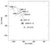 |
Fig. A.1 Relative position of the FUor component with respect to the Herbig from measurements. Labels report year:month of observation (see text for the references). The red point refers to our SPHERE observations. |
Appendix C: Flux calibration of the [O i] image
To perform the flux calibration of the [O i] image, we first calibrated the Cnt_Ha image using the conversion coefficient reported by Schmid et al. (in prep.), assuming a 10% uncertainty on the provided factor. To check the goodness of this calibration, we derived an estimate of the binary integrated R-band magnitude by measuring the counts in a circular aperture including both components. We thus obtain R = 8.5 ± 0.2 mag for the binary. The measured magnitude is consistent with the integrated magnitudes of V = 9.3 and IC = 8.0 reported by the Kamogata Wide-field Survey on 30 Mar. 2015 (Maehara & Ukita 2015), i.e. the night before our SPHERE observations, also considering that the typical photometric variability of Z CMa on a timescale of one day is below 0.1 mag.
To flux calibrate the [O i] image, we then made the assumption that the continuum flux density in the Cnt_Ha image (at λ = 645 nm) is the same for the [O i] image (at λ = 630 nm). On this basis, we were able to derive a count-to-flux conversion factor for the [O i] image by considering a circular area centred on the SE component on both images. We selected the FUor because we expect a weaker on-source [O i] line emission on this component than on the Herbig star. Using different radii for the circular aperture we derive conversion factors that differ for less than 2%. To be conservative, also considering the previous continuum flux density assumption, we associate a relative uncertainty of 10% on the computed factor. This, in conjunction with the initial uncertainty on the Cnt_Ha image conversion coefficient, allows us to evaluate an accuracy of 20% for the flux calibration of the [O i] image.
All Figures
|
Fig. 1 a)Continuum-subtracted (top) and deconvolved (bottom) [O i] images of the Z CMa system. The deconvolved image shows only the diffuse emission as reconstructed by the MC-RL algorithm. The centroids of the two stars and the position of the main knots of the FUor jet are indicated. Areas heavily corrupted by artefacts around the star centroids have been masked. b) Same for the Hα observations. c) Fitted transverse positions of the peak of the FUor jet spatial profile as a function of the distance from the exciting source for both the [O i] continuum-subtracted (blue squares) and deconvolved images (red circles). Blue crosses and red pluses indicate the measured profile width of the two images. The solid green line is the best fit of the wiggle produced by an orbital motion of the jet source around a companion (Anglada et al. 2007) to the peaks of the continuum-subtracted image. |
| In the text | |
|
Fig. A.1 Relative position of the FUor component with respect to the Herbig from measurements. Labels report year:month of observation (see text for the references). The red point refers to our SPHERE observations. |
| In the text | |
Current usage metrics show cumulative count of Article Views (full-text article views including HTML views, PDF and ePub downloads, according to the available data) and Abstracts Views on Vision4Press platform.
Data correspond to usage on the plateform after 2015. The current usage metrics is available 48-96 hours after online publication and is updated daily on week days.
Initial download of the metrics may take a while.