© ESO, 2016

1. Introduction

He-rich white dwarfs with metals are classified as DBZ and, at low temperature, they are DZ. Recent key observations with Spitzer and Hubble space telescopes have given us real insights into the composition of extra-solar planetary systems through the spectroscopic detection of traces of heavy metal in cool DZ white dwarf atmospheres. These observed features are now attributed to the presence of rocky planetary material like asteroids that previously orbited these stars. They could play a central role in characterizing the chemistry of this rocky material. The analysis of DZ spectra is therefore a potentially valuable method for determining the existence in the stellar progenitor of exoplanetary systems and their chemical abundances (see Farihi 2016, and references therein).

The construction of model atmospheres and synthetic spectra for DZ white dwarfs is necessary to derive reliable atmospheric parameters and the surface chemical composition for these objects. In the absence of hydrogen, the effect of all other opacity sources on the structure of the atmosphere is significantly enhanced. The omission of opacity results in systematic errors in the predicted flux distribution and hence in the effective temperature. This is a major concern for the calculation of model atmospheres. Heber & Schoenberner (1981) introduced the blanketing effect of strong ultraviolet metal lines. The methods to include all the broadened lines remain misleading, a reliance on simplified models of van der Waals quasi-static line broadening (see Koester et al. 2011, and references therein). These recipes are widely in use in model atmospheres, the broadening constants C₆ being determined following Unsold (1955). As noted by Koester et al. (2011), Zeidler-K.T. et al. (1986) studied line blanketing and metal abundances in helium-rich white dwarf atmospheres. They noted that, with the low electron densities being present, line broadening is dominated by collision broadening with neutral He. Initial assumptions of C₆ based on the methods of Unsold (1955) and others led to inconsistencies in the model spectra, strikingly in the observed absence of weak Mg lines that should have been present at the abundances required to match the resonance lines. They found that, by artificially increasing C₆ by an order of magnitude, they could reproduce the observed spectra. However, even with that ad hoc choice, discrepancies in the core and wing of Mg II lines could not be removed.

The shift of the line arises from the long-range part of potentials and the far line wings of the broadened lines exhibit characteristics that arise at short range. In a first approximation, van der Waals potentials describe the long-range part of the potentials. However, it is most important that accurate molecular potentials be involved in the calculations of line broadening and opacities for radiative transitions. Line broadening of the Ca⁺ and Mg⁺ resonance lines in presence of He have been studied by Bottcher et al. (1975) and Monteiro et al. (1986) using model potential curves. In this work we consider the broadening of Mg⁺ by He to develop an accurate treatment of the resonance lines, including the very far wing that enables correct calculations of radiative transport in DZ white dwarfs.

For that purpose, intensive ab initio calculations have been performed to obtain the ground and first excited potential energy curves (PECs) for the Mg⁺–He system. We report and compare the results of two different methods to compute ab initio Mg⁺He interaction potentials (Sect. 2). A reliable determination of the line profiles that is applicable in all parts of the line at all densities is the Anderson semi-classical unified theory, which utilizes the Fourier transform of an autocorrelation function (Anderson 1952) (Sect. 3). This paper is a continuation of our studies of sodium and ionized Ca resonance lines perturbed by He (Allard 2013; Allard & Alekseev 2014; Allard et al. 2014a). We illustrate the evolution of the absorption spectra of Mg⁺-He collisional profiles for the densities (Sect. 3.1) and the temperatures (Sect. 3.2) prevailing in the atmosphere of cool white dwarf stars. The calculations span the range 4000 K to 12 000 K. Moreover, the impact approximation determines the asymptotic behavior of the unified line shape autocorrelation function. The dependence of the impact line parameters on temperature is presented in Sect. 4. In this way, the results described here are applicable to a more general line profile and opacity evaluation for the same perturbers at any given layer in the photosphere.

2. Mg⁺He diatomic potentials

Line profile intensities are functions of both excited and ground state interactions and consequently a precise determination of the electronic energies, as well as optical transition dipole moments, are crucial to compute accurate line profiles for the whole wavelength range. In this section, we report on and compare the results of two different methods to compute ab initio Mg⁺He interaction potentials.

2.1. CASSCF-CASPT2 calculations

Calculations were performed by one of us (hereafter VA) using MOLCAS 7.6 (Aquilante et al. 2010). Energies with the inclusion of the static contribution of electron correlation energy were calculated at the CASSCF (complete active space self-consistent field) level. Calculations of the dynamic electron correlation effects for the multiconfigurational CASSCF wave functions are based on the second order perturbation theory, the CASPT2 method in MOLCAS (Finley et al. 1998). The CASSCF-CASPT2 energies and wave functions are further used to obtain adiabatic energies with the inclusion of the spin-orbit interaction using the state interaction program RASSI (restricted active space state interaction) in MOLCAS (Malmqvist et al. 2002). The RASSI program also calculates dipole moments of optical transitions between electronic states.

Calculations were performed using relativistic atomic natural orbital (ANO) type basis sets (Almlöf & Taylor 1987). The potentials shown in Fig. 1 were obtained with Mg.ano-rcc.Roos.17s12p6d2f2g.9s8p6d2f2g, He.ano-rcc.Widmark.9s4p3d2f.7s4p3d2f, which are the largest ANO-type basis sets in the MOLCAS basis set library. The accuracy of CASSCF-CASPT2-RASSI calculations with the ANO basis sets has been discussed in detail in Roos et al. (2004). Smaller ANO-type basis sets for the He atom (VQZP and VTZP) were tested as well. The deviations from the results obtained with the largest basis sets were found to be rather small (at least the differences would not be seen in the scale of Fig. 1). The asymptotic energies were adjusted to match the energies of the Mg⁺(3p²P_{1 / 2, 3 / 2}) doublet.

Calculations were performed in the C₁ symmetry for an active space consisting of the five lowest in energy unoccupied orbitals, including the singly occupied valence 2p⁶3s orbital. This selection of active space yields electronic states of the Mg⁺He molecule, which correlate with the ground 2p⁶3s and excited 3p and 4s states of the Mg⁺ ion. The interaction of Mg 2p⁶3p with He provides ${}^{\mathrm{2}}\mathrm{\Pi }_{\mathrm{1}\mathit{/}\mathrm{2}\mathit{,}\mathrm{3}\mathit{/}\mathrm{2}}$ states, and a ²Σ state. A slight difference between the ${}^{\mathrm{2}}\mathrm{\Pi }_{\mathrm{1}\mathit{/}\mathrm{2}}$ and ${}^{\mathrm{2}}\mathrm{\Pi }_{\mathrm{3}\mathit{/}\mathrm{2}}$ states is not seen in the scale of Fig. 1. The dipole moment of 3s²Σ→ 3p²Π transitions is nearly constant. The 3p²Σ state interacts with a higher lying 4s²Σ state. Owing to this interaction, the dipole moment of the resonance 3s ²Σ→ 3 p²Σ transition decreases (Fig. 3), while the asymptotically forbidden 3s²Σ⁺→ 4s²Σ⁺ transition acquires some strength as R decreases.

2.2. CASSCF-MRCI calculations

The improvement over the previous molecular data described above consists in a more accurate determination of the intermediate and long-range part of the Mg⁺-He potential. The potential energy curves were computed over a large range of intermolecular distances, namely, from 2.0 to 200.0 au, allowing a good description of the spectral line core. This is important when determining the absorption spectra of Mg⁺-He obtained at low He density. All new ab initio calculations have been performed by one of us (hereafter GG) using the MOLPRO package (Werner et al. 2012). The dimer ground state emerges from the ion Mg⁺ itself in its ground state [Ne]3s¹²P and has Σ symmetry (noted X²Σ), while the lowest two excited states come from the first excited state of Mg⁺. One has Π symmetry (e.g. A ²Π) and presents a very deep and narrow well, at short range, and the other is of a pure anti-bonding type with Σ symmetry (e.g. B ²Σ). We have computed adiabatic potential energy curves (PECs) for the ground state and the first two excited states of Mg⁺ + He. To this end, we have used a high level ab initio method, namely the state-averaged complete active space self-consistent field-multireference configuration interaction (SA-CASSCF-MRCI).

In view of the small mass of Mg, all scalar relativistic effects have been neglected at this point. MRCI calculations based on reference functions obtained from the state-averaged complete active space self-consistent field (SA-CASSCF) method are performed to get the best possible accuracy on the first excited states’ energies. The active space used in the SA-CASSCF method contains five σ-type and four π-type molecular orbitals. The former correlate asymptotically to the Mg⁺:3s, 3p₀ and He:1s, 2s, 2p₀ atomic orbitals, the latter to the Mg⁺:3p₁, 3p_-1 and He:2p₁, 2p_-1 atomic orbitals. All electrons were dynamically included in the calculations.

For the ion Mg⁺, since a good description of the core is necessary, we used the core-valence aug-cc-pCVQZ basis set, which possesses additional tight functions, with contraction scheme (20s, 16p, 7d, 5f, 3g) −→ (10s, 9p, 7d, 5f, 3g). To describe the He atom, we used the aug-cc-pV6Z basis set, formed using 186 primitive functions with contraction scheme (11s, 6p, 5d, 4f, 3g, 2h) −→ [7s, 6p, 5d, 4f, 3g, 2h]. The use of such an extended basis set is expected to provide results for atomic and molecular properties very close to the complete basis set limit and to dramatically reduce the basis set superposition errors, which have already been corrected with the usual counterpoise method (Boys & Bernardi 1970). To correct for the lack of size-consistency of the MRCI method, we used the Davidson cluster-corrected total energies (Davidson & Silver 1977) within the realm of the supermolecule approach to obtain complexation energies.

The ab initio data points obtained have been fitted to an RKHS kernel, as described in Ho & Rabitz (1996). These analytic forms of the adiabatic PECs allow a proper description of the long range part of the potential. In particular, the ground state interaction of Mg⁺He is correctly described as behaving asymptotically in r^-4, as it should for a charge-induced dipole system.

The electrostatic interaction between Mg⁺ and He is much stronger than that between Mg and He, owing to the ionic character of Mg⁺, with a well for the ground state roughly 14 times deeper than that of its neutral conterpart MgHe. As a result, the X²Σ state presents a well depth D_e of roughly −68.0 cm^-1 at an internuclear distance r_e = 6.7 a.u., which are values close to those obtained earlier (D_e = −73.2 cm^-1 and r_e = 6.6 a.u.) by Gardner et al. (2010). The A²Π state exhibits a narrow well 2267 cm^-1 deep at r_e = 3.5 a.u.

Also, the Russel-Saunders spin-orbit coupling in the ion Mg⁺ (Δ_SO = 91.57 cm^-1) is comparable to that of the Na atom (Δ_SO = 17.20 cm^-1) (Dell’Angelo et al. 2012; Allard et al. 2014b), but still roughly five times larger. However, we make the hypothesis that the effect of the value of the atomic Mg⁺ spin-orbit coupling parameter Δ_SO only varies slowly when the Mg⁺ ion and He atom approach one another. In this way, we avoid computations of its variation with internuclear distance, which could be done using relativistic electronic structure calculations, or at least relativistically-based corrections. The incorporation of the Russel-Saunders Mg⁺ spin-orbit coupling at all internuclear distances, starting from the adiabatic PECs, is then realized following the lines described in Cohen & Schneider (1974).

Figures 1 and 2 show the potential energy curves obtained with MRCI calculations, which will be used in the line profile calculations presented in the paper. ${\mathit{V}}_{\mathit{e}}\mathrm{\left[}\mathit{R}\mathrm{\right(}\mathit{t}\mathrm{\left)}\mathrm{\right]}\mathrm{=}{\mathit{E}}_{\mathit{e}}\mathrm{\left[}\mathit{R}\mathrm{\right(}\mathit{t}\mathrm{\left)}\mathrm{\right]}\mathrm{-}{\mathit{E}}_{\mathit{e}}^{\mathrm{\infty }}\mathit{.}$(1)The potentials obtained in CASPT2 and MRCI calculations are overplotted in Fig. 1. As can be seen, the results of these two methods are in a good agreement at short internuclear distance.

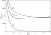Fig. 1 Short-range part of the potential curves for the 3s and 3p states of the Mg+He molecule of GG (black lines) compared to VA (green dotted lines).

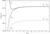Fig. 2 Long range part of the GG potential curves correlated with 3p states. ${}^{\mathrm{2}}\mathrm{\Sigma }_{\mathrm{1}\mathit{/}\mathrm{2}}$ (full line), ${}^{\mathrm{2}}\mathrm{\Pi }_{\mathrm{3}\mathit{/}\mathrm{2}}$ (dashed line) and ${}^{\mathrm{2}}\mathrm{\Pi }_{\mathrm{1}\mathit{/}\mathrm{2}}$ (dotted line).

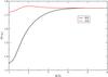Fig. 3 Dipole moments for the 3 s → 3 ptransitions in Mg+He molecule (CASSCF–CASPT2 calculations).

3. Absorption spectra for cool white dwarfs

In a previous paper (Allard et al. 1999), we derived a classical path expression for a pressure-broadened atomic spectral line shape that allows for an electric dipole moment that is dependent on the position of perturbers, which is not included in the more usual approximation of Anderson (1952) and Baranger (1958b,a). When broadened by helium, absorption coefficients of ionized magnesium resonance lines arising from 3s to 3p transition depend on di-molecule potentials composed of Mg⁺ and He (Figs. 1, 2) and dipole moments (Fig. 3).

The spectrum, I(Δω), is the Fourier transform (FT) of the dipole autocorrelation function, Φ(s). This is given by $\mathit{I}\mathrm{\left(}\mathrm{\Delta }\mathit{\omega }\mathrm{\right)}\mathrm{=}\frac{\mathrm{1}}{\mathit{\pi }}\hspace{0.17em}\mathit{Re}\hspace{0.17em}{\mathrm{\int }}_{\mathrm{0}}^{\mathrm{+}\mathrm{\infty }}\mathrm{\Phi }\mathrm{\left(}\mathit{s}\mathrm{\right)}{\mathrm{e}}^{\mathrm{-}\mathrm{i\Delta }\mathit{\omega s}}\mathrm{d}\mathit{s}\mathit{.}$(2)A pairwise additive assumption allows us to calculate I(Δω), when N perturbers interact as the FT of the Nth power of the autocorrelation function φ(s) of a unique atom-perturber pair. For a perturber density n_p, we obtain $\mathrm{\Phi }\mathrm{\left(}\mathit{s}\mathrm{\right)}\mathrm{=}{\mathrm{e}}^{\mathrm{-}{\mathit{n}}_{\mathrm{p}}\mathit{g}\mathrm{\left(}\mathit{s}\mathrm{\right)}}\mathit{,}$(3)where the decay of the autocorrelation function with time leads to atomic line broadening.

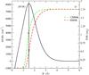Fig. 4 Variation with temperature in the modulated dipole and the difference potential of the B-X states of Mg+-He molecule.

For a transition α = (i,f) from an initial state i to a final state f, we have $\begin{array}{ccc}{\mathit{g}}_{\mathit{\alpha }}\mathrm{\left(}\mathit{s}\mathrm{\right)}& \mathrm{=}& \frac{\mathrm{1}}{{\sum }_{\mathit{e,}{\mathit{e}}^{\mathrm{\prime }}}\hspace{0.17em}\mathrm{\left(}\mathit{\alpha }\mathrm{\right)}\hspace{0.17em}\mathrm{|}{\mathit{d}}_{\mathit{e}{\mathit{e}}^{\mathrm{\prime }}}{\mathrm{|}}^{\mathrm{2}}}\sum _{\mathit{e,}{\mathit{e}}^{\mathrm{\prime }}}\hspace{0.17em}\mathrm{\left(}\mathit{\alpha }\mathrm{\right)}\\ & & \mathrm{\times }{\mathrm{\int }}_{\mathrm{0}}^{\mathrm{+}\mathrm{\infty }}\mathrm{2}\mathit{\pi \rho d\rho }{\mathrm{\int }}_{\mathrm{-}\mathrm{\infty }}^{\mathrm{+}\mathrm{\infty }}\mathrm{d}\mathit{x}\begin{array}{c}\mathrm{˜}\\ {\mathit{d}}_{\mathit{e}{\mathit{e}}^{\mathrm{\prime }}}\end{array}\mathrm{\left[}\hspace{0.17em}\mathit{R}\mathrm{\right(}\mathrm{0}\mathrm{\left)}\hspace{0.17em}\mathrm{\right]}\hspace{0.17em}\\ & & \end{array}$(4)In Eq. (4), e and e′ label the energy surfaces on which the interacting atoms approach the initial and final atomic states of the transition. The sum ${\sum }_{\mathit{e,}{\mathit{e}}^{\mathrm{\prime }}}^{\mathrm{\left(}\mathit{\alpha }\mathrm{\right)}}$ is over all pairs (e,e′) such that ω_e′,e(R) → ω_α as R → ∞.

For a more direct comparison of the contributions of the two fine-structure components of the doublet, it is convenient to use a cross-section σ associated with each component. The relationship between the computed cross-section and the normalized absorption coefficient given in Eq. (2) is $\mathit{I}\mathrm{\left(}\mathrm{\Delta }\mathit{\omega }\mathrm{\right)}\mathrm{=}\mathit{\sigma }\mathrm{\left(}\mathrm{\Delta }\mathit{\omega }\mathrm{\right)}\mathit{/}\mathit{\pi }{\mathit{r}}_{\mathrm{0}}\mathit{f,}$(5)where r₀ is the classical radius of the electron, and f is the oscillator strength of the transition.

In the sections which follow, we review the meaning of these terms in Eq. (4) and the data we use to evaluate the absorption line shape of ionized magnesium resonance lines in dense helium.

3.1. Satellite bands and density dependence

In the present context, the perturbation of the frequency of the atomic transition during the collision results in a phase shift, η(s), which is calculated along a classical path R(t) that is assumed to be rectilinear. The phase shift

$\mathit{\eta }\mathrm{\left(}\mathit{s}\mathrm{\right)}\mathrm{=}\frac{\mathit{i}}{ħ}{\mathrm{\int }}_{\mathrm{0}}^{\mathit{s}}\hspace{0.17em}\mathrm{d}\mathit{t}{\mathit{V}}_{{\mathit{e}}^{\mathrm{\prime }}\mathit{e}}\mathrm{[}\hspace{0.17em}\mathit{R}\mathrm{(}\mathit{t}\mathrm{)}\hspace{0.17em}\mathrm{]}\mathit{,}$(6)where ΔV(R) represents the difference between the electronic energies of the quasimolecular transition. The potential energy for a state e is

$\begin{array}{ccc}& & {\mathit{V}}_{\mathit{e}}\mathrm{\left[}\mathit{R}\mathrm{\right(}\mathit{t}\mathrm{\left)}\mathrm{\right]}\mathrm{=}{\mathit{E}}_{\mathit{e}}\mathrm{\left[}\mathit{R}\mathrm{\right(}\mathit{t}\mathrm{\left)}\mathrm{\right]}\mathrm{-}{\mathit{E}}_{\mathrm{e}}^{\mathrm{\infty }}\mathit{.}\\ & & \mathrm{\Delta }\mathit{V}\mathrm{\left(}\mathit{R}\mathrm{\right)}\mathrm{\equiv }{\mathit{V}}_{{\mathit{e}}^{\mathrm{\prime }}\mathit{e}}\mathrm{\left[}\mathit{R}\mathrm{\right(}\mathit{t}\mathrm{\left)}\mathrm{\right]}\mathrm{=}{\mathit{V}}_{{\mathit{e}}^{\mathrm{\prime }}}\mathrm{\left[}\mathit{R}\mathrm{\right(}\mathit{t}\mathrm{\left)}\mathrm{\right]}\mathrm{-}{\mathit{V}}_{\mathit{e}}\mathrm{\left[}\mathit{R}\mathrm{\right(}\mathit{t}\mathrm{\left)}\mathrm{\right]}\mathit{.}\end{array}$At time t from the point of closest approach $\mathit{R}\mathrm{\left(}\mathit{t}\mathrm{\right)}\mathrm{=}{\mathrm{[}{\mathit{\rho }}^{\mathrm{2}}\mathrm{+}\mathrm{(}\mathit{x}\mathrm{+}\mathit{v̅}\mathit{t}{\mathrm{)}}^{\mathrm{2}}\mathrm{]}}^{\mathrm{1}\mathit{/}\mathrm{2}}\mathit{,}$(9)with ρ the impact parameter of the perturber trajectory and x the position of the perturber along its trajectory at time t = 0.

We see from the potentials in Fig. 2 that two excited molecular levels, ${}^{\mathrm{2}}\mathrm{\Sigma }_{\mathrm{1}\mathit{/}\mathrm{2}}$ and ${}^{\mathrm{2}}\mathrm{\Pi }_{\mathrm{3}\mathit{/}\mathrm{2}}$, contribute to the P_{3 / 2} line and that they produce opposite wings (Fig. 5). The ${}^{\mathrm{2}}\mathrm{\Pi }_{\mathrm{1}\mathit{/}\mathrm{2}}$ state that determines the P_{1 / 2} line radiates solely in the red wing, and as a consequence the P_{1 / 2} line, is strongly asymmetric to the red (Fig. 6).

Owing to the interaction between Mg⁺ and He atoms, the far line wings of the broadened lines exhibit characteristics of molecular spectra. The potential difference ΔV related to the 3s ²Σ_{1 / 2} → 3p ²Σ_{1 / 2}transition, for the Mg⁺-He pair, has a maximum ΔV_max = 8100 cm^-1 at very short distance R = 1.5 Å (Fig. 4). The unified theory (Anderson 1952; Allard 1978; Royer 1978) predicts that there will be quasi-molecular line satellites centered periodically at frequencies corresponding to the extrema of the difference potential. In the far blue wing, a notable feature is the primary peak that occurs at 0.23 μm (Fig. 5), corresponding to that large maximum of ΔV. While, in the case of the triplet 3p−4s Mg lines, a satellite band located in the near blue wing is responsible of a blue asymmetry of the core of the lines. This asymmetry is a consequence of lower maxima (400 cm^-1) in the corresponding Mg-He potential energy difference curves (Leininger et al. 2015; Allard et al. 2016a).

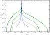Fig. 5 Variation with He atom density of the P3/2 component at T = 6000 K. GG potentials (black curves), VA potentials (green curves). From top to bottom nHe = 1022, 1021, and 1020 cm-3. The corresponding Lorentzian profile for nHe = 1020 cm-3 is overplotted (blue line).

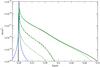Fig. 6 Variation with He atom density of the P1 / 2 component at T = 6000 K. GG potentials (black curves), VA potentials (green curves). From top to bottom nHe = 1022, 1021, and 1020 cm-3. The corresponding Lorentzian profile for nHe = 1020 cm-3 is overplotted (blue line).

If one assumes additive-pair interactions, the satellite feature at ΔV_max in the binary spectrum will also appear in the spectrum at integer multiples of ΔV_max owing to the presence of additional perturbers in the collision volume . When the helium density reaches 10²¹ cm^-3, a second satellite corresponding to 2ΔV_max appears as a shoulder (Fig. 5). The blue wing of the P_1/2 component decreases very rapidly because of the shape of the potential of the A ²Π_{1 / 2} state. While the red wings of the two components P_{1 / 2,3 / 2} extend until 1200 Å and more from the line center for the helium density greater than 10²¹ cm^-3, the line wings are mostly formed in the lower photosphere, where higher helium density should prevail. At these high densities, the one-perturber binary collision approximation is not valid because the probability of an Mg⁺ collision with two perturbers is larger than the probability of a collision with only one (Allard 1978; Royer 1978; Kielkopf & Allard 1979). The density effect on the core of the lines is also very significant when the He density becomes larger than 10²¹ cm^-3. Figure 7 shows that the Lorentzian gives a rather good description of the core until n_He = 10²¹ atoms cm^-3, when the density is as high as n_He = 2 × 10²¹, the impact approximation is no more valid, even in the core of the line. The line shapes of the core of the doublet are no longer Lorentzian. The line parameters of the Lorentzians plotted in Figs. 5−7 are obtained in the impact approximation (see Sect. 4) using new ab initio potentials (Figs. 1 and 2).

A comparison of the absorption cross-sections for 3s−3p P_3/2 and 3s−3p P_1/2 transitions computed using VA potentials are shown in Figs. 5, 6. The agreement of the molecular data at short distance (Fig. 1), mainly in the slope of the repulsive walls, leads to this close agreement in the line wings and the prediction of the quasi-molecular line satellite at 0.23 μm. In Allard et al. (2007c), we have shown that ab initio K-H₂ potentials systematically less repulsive than the pseudo-potentials of Rossi & Pascale (1985) allowed a K-H₂ quasi-molecular line satellite to be predicted, which closely matches the position and shape of an observed feature in the spectrum of the T1 dwarf ε Indi Ba (Allard et al. 2007a). More recently, in Allard et al. (2016b), the position of the predicted line satellite was confirmed by a laboratory measurement.

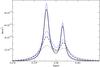Fig. 7 Variation of the absorption cross-section in the central part of the sum of the components P3 / 2 and P1 / 2 with the He density, (from top to bottom nHe = 1, 2 and, 3 × 1021 cm-3, T = 8000 K). The corresponding sum of Lorentzian profiles for nHe = 1 and, 2 × 1021 cm-3 is overplotted (blue lines).

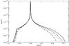Fig. 8 Variation of the absorption cross-section of the sum of the components P3 / 2 and P1 / 2 with temperature, (from top to bottom T = 12 000, 8000, 6000 and 4000 K, nHe = 1021 cm-3).

3.2. Temperature dependence

In Fig. 8 we show the absorption cross-section for the sum of the components of the resonance line of Mg⁺ for a He density of 10²¹ cm^-3 and temperatures from 4000 to 12 000 K. The strength and extension of the line wings are very temperature sensitive. In Eq. (4) we define $\begin{array}{c}{}_{\mathrm{˜}}\\ {\mathit{d}}_{\mathit{e}{\mathit{e}}^{\mathrm{\prime }}}\end{array}\mathrm{\left(}\mathit{R}\mathrm{\right(}\mathit{t}\mathrm{\left)}\mathrm{\right)}$ as a modulated moment dipole (Allard et al. 1999) $\mathit{D}\mathrm{\left(}\mathit{R}\mathrm{\right)}\mathrm{\equiv }\begin{array}{c}\mathrm{˜}\\ {\mathit{d}}_{\mathit{e}{\mathit{e}}^{\mathrm{\prime }}}\end{array}\mathrm{\left[}\mathit{R}\mathrm{\right(}\mathit{t}\mathrm{\left)}\mathrm{\right]}\mathrm{=}{\mathit{d}}_{\mathit{e}{\mathit{e}}^{\mathrm{\prime }}}\mathrm{\left[}\mathit{R}\mathrm{\right(}\mathit{t}\mathrm{\left)}\mathrm{\right]}{\mathrm{e}}^{\mathrm{-}\frac{\mathit{\beta }}{\mathrm{2}}{\mathit{V}}_{\mathit{e}}\mathrm{\left[}\mathit{R}\mathrm{\right(}\mathit{t}\mathrm{\left)}\mathrm{\right]}}\mathit{,}$(10)where β is the inverse temperature (1 /kT). The transition dipole moments d_ee′(R) have been calculated by VA (Fig. 3). Here V_e is the ground state potential X ²Σ because we consider absorption transitions from the lower molecular state. The strength of the line satellite at about 0.23 μm increases with temperature (Fig. 8). The line wing amplitude depends on the value of the electric transition dipole moment in the internuclear region where the line wing is formed. In particular the presence and amplitude of line satellites are very sensitive to the temperature owing to the fast variation of the modulated dipole moment with temperature in the internuclear region, where the line satellite is formed (Fig. 4). This explains why the second line satellite appears distinctly at 12 000 K as a change in the slope on the blue wing.

From this dependence, it is apparent that the sensitivity of the line wings to pressure and temperature is a tool for determining basic parameters of white dwarf atmospheres, provided that the physics underlying its formation is well described. In the next section, we examine the dependence of the line parameters on the temperature.

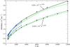Fig. 9 Variation with temperature of the half-width at half-maximum of the 3P3 / 2–3s (full line) and 3P1 / 2–3s (dashed line) resonance lines of Mg+ perturbed by He collisions. GG potentials (black curves), VA potentials (green curves), and model potentials of Monteiro et al. (1986; blue curves). The rates are in units of 10-9 rad s-1.

4. Line core parameters

Pressure broadening by helium is one of the major broadening mechanisms in the atmosphere of DZ white dwarfs. Since the resulting line profile in a model atmosphere calculation is the integration of the flux in all layers from the deepest to the uppermost, it is important that the centers are adequately represented, i.e. they can be non-Lorentzian at high densities of the innermost layers, while Lorentzian in the upper atmosphere. However, they are characterized by different widths than were predicted by the hydrogenic van der Waals approximation, which is usually used for the cores, as was emphasized by Allard et al. (2007b) and Peach (2011). At sufficiently low densities of perturbers, the symmetric center of a spectral line is Lorentzian and can be defined by two line parameters, the width and the shift of the main line. These quantities can be obtained in the impact limit (s → ∞) of the general calculation of the autocorrelation function (Eq. (4)). For He density below n_He = 10²⁰ atoms cm^-3, the core of the line is described adequately by a Lorentzian (Figs. 5, 6). The line widths w (HWHM) are linearly dependent on He density, and a power law in temperature given for the ${}^{\mathrm{2}}\mathit{P}_{\mathrm{1}\mathit{/}\mathrm{2}}$ transition by $\mathit{w}\mathrm{=}\mathrm{0.055}\mathrm{\times }{\mathrm{10}}^{-9}{\mathit{n}}_{\mathrm{He}}\hspace{0.17em}{\mathit{T}}^{\mathrm{0.4309}}\mathit{,}$(11)and for the ${}^{\mathrm{2}}\mathrm{P}_{\mathrm{3}\mathit{/}\mathrm{2}}$ transition by $\mathit{w}\mathrm{=}\mathrm{0.09}\mathrm{\times }{\mathrm{10}}^{-9}{\mathit{n}}_{\mathrm{He}}\hspace{0.17em}{\mathit{T}}^{\mathrm{0.4031}}\mathit{.}$(12)The non-linear dependence on temperature is illustrated in Fig. 9. These expressions may be used to compute the widths for temperatures of stellar atmospheres from 400 to at least 12 000 K.

We are not aware of the laboratory measurements of spectra of Mg⁺ under the conditions of high density and temperature needed for comparison with the calculations here. One set of experimental width and shift is available at lower temperature, T = 556 K by Giles & Lewis (1982) (Table 1). We undertook a comparison between calculated line parameters using different potentials and different theoretical approaches. In Fig. 9, we plotted the results obtained in the semi-classical unified theory using the VA potentials presented in Fig. 1. We notice that there is a rather good agreement of the results obtained with the GG potentials to those obtained by VA for the two components of the resonance line. Model potential curves for low-lying Σ and Π states of the Ca⁺-He and Mg⁺-He systems were calculated and used to obtain fully quantal broadening and shift parameters for the Ca⁺ 4p ²P_{1 / 2,3 / 2}–4s ²S_{1 / 2} and Mg⁺ 3p P_{1 / 2,3 / 2}–3s ²S_{1 / 2} spectral lines for a range of temperatures 400−3000 K. The broadening and shift parameters for Mg⁺ and Ca⁺ are given in Table 6 of Monteiro et al. (1986). In Fig. 9, we reported the temperature-dependence of the width of Mg⁺ 3p P_{1 / 2,3 / 2}–3s ²S_{1 / 2}. The widths were found to increase as T^α, α taking the values 0.42 and 0.36 for the Mg⁺P = 1 / 2 and P = 3 / 2. A comparison between the experimental value at T = 556 K and the theoretical values is given in Table 1, with the experimental uncertainties given in brackets.

This study shows the sensitivity of the line parameters to the potentials.

5. Conclusions

The atmospheres of DZ white dwarfs are almost pure helium. The accurate treatment of the Mg⁺ resonance lines should strongly influence the predicted spectrum, as in the case of the triplet 3p–4s Mg lines (Allard et al. 2016a). This requires the knowledge of accurate line profiles under the physical conditions of the atmospheres of cool DZ white dwarfs. Many of the problems in collision-induced radiative transitions have been solved within the one-perturber approximation. At very low densities, the binary model for an optically active atom in collision with one perturber is valid for the whole profile, except for the central part of the line. In very cool white dwarfs, the perturber density n_He is so high that the one-perturber approximation breaks down. When the He density is greater than n_He = 10²⁰ atoms cm^-3, the far wing of the P_{3 / 2} and P_{1 / 2} components of the resonance lines is due to multiple-perturber collisions, which are included in the theory and models described here. Experimental laboratory tests are planned to re-determine the low density and low temperature line core shift and width as a test of the long range potential. The test will also help identify distinctive characteristics of the line wings at high density as a test of the stronger, shorter range, interactions that are used for the theoretical models. In conclusion, complete unified line profiles based on accurate atomic and molecular physics should be incorporated into the analysis of cool DZ white dwarf spectra. They should provide a good fit of UV MgII resonance lines without an unphysical increase of the van der Waals constant C₆, as in Koester & Wolff (2000). Moreover the correct determination of the line parameters should allow a good description of the spectral line core.

References

All Tables

All Figures

	Fig. 1 Short-range part of the potential curves for the 3s and 3p states of the Mg+He molecule of GG (black lines) compared to VA (green dotted lines).
In the text

	Fig. 2 Long range part of the GG potential curves correlated with 3p states. ${}^{\mathrm{2}}\mathrm{\Sigma }_{\mathrm{1}\mathit{/}\mathrm{2}}$ (full line), ${}^{\mathrm{2}}\mathrm{\Pi }_{\mathrm{3}\mathit{/}\mathrm{2}}$ (dashed line) and ${}^{\mathrm{2}}\mathrm{\Pi }_{\mathrm{1}\mathit{/}\mathrm{2}}$ (dotted line).
In the text

	Fig. 3 Dipole moments for the 3 s → 3 ptransitions in Mg+He molecule (CASSCF–CASPT2 calculations).
In the text

	Fig. 4 Variation with temperature in the modulated dipole and the difference potential of the B-X states of Mg+-He molecule.
In the text

	Fig. 5 Variation with He atom density of the P3/2 component at T = 6000 K. GG potentials (black curves), VA potentials (green curves). From top to bottom nHe = 1022, 1021, and 1020 cm-3. The corresponding Lorentzian profile for nHe = 1020 cm-3 is overplotted (blue line).
In the text

	Fig. 6 Variation with He atom density of the P1 / 2 component at T = 6000 K. GG potentials (black curves), VA potentials (green curves). From top to bottom nHe = 1022, 1021, and 1020 cm-3. The corresponding Lorentzian profile for nHe = 1020 cm-3 is overplotted (blue line).
In the text

	Fig. 7 Variation of the absorption cross-section in the central part of the sum of the components P3 / 2 and P1 / 2 with the He density, (from top to bottom nHe = 1, 2 and, 3 × 1021 cm-3, T = 8000 K). The corresponding sum of Lorentzian profiles for nHe = 1 and, 2 × 1021 cm-3 is overplotted (blue lines).
In the text

	Fig. 8 Variation of the absorption cross-section of the sum of the components P3 / 2 and P1 / 2 with temperature, (from top to bottom T = 12 000, 8000, 6000 and 4000 K, nHe = 1021 cm-3).
In the text

	Fig. 9 Variation with temperature of the half-width at half-maximum of the 3P3 / 2–3s (full line) and 3P1 / 2–3s (dashed line) resonance lines of Mg+ perturbed by He collisions. GG potentials (black curves), VA potentials (green curves), and model potentials of Monteiro et al. (1986; blue curves). The rates are in units of 10-9 rad s-1.
In the text

References

- Allard, N. F. 1978, J. Phys. B: At. Mol. Opt. Phys., 11, 1383 [Google Scholar]
- Allard, N. F. 2013, in EAS Pub. Ser., 63, 403 [Google Scholar]
- Allard, N. F., & Alekseev, V. A. 2014, Adv. Space Res., 54, 1248 [NASA ADS] [CrossRef] [Google Scholar]
- Allard, N. F., Royer, A., Kielkopf, J. F., & Feautrier, N. 1999, Phys. Rev. A, 60, 1021 [NASA ADS] [CrossRef] [Google Scholar]
- Allard, F., Allard, N. F., Homeier, D., et al. 2007a, A&A, 474, L21 [NASA ADS] [CrossRef] [EDP Sciences] [Google Scholar]
- Allard, N. F., Kielkopf, J. F., & Allard, F. 2007b, EPJ D, 44, 507 [Google Scholar]
- Allard, N. F., Spiegelman, F., & Kielkopf, J. F. 2007c, A&A, 465, 1085 [NASA ADS] [CrossRef] [EDP Sciences] [Google Scholar]
- Allard, N. F., Homeier, D., Guillon, G., Viel, A., & Kielkopf, J. 2014a, J. Phys. Conf. Ser., 548, 012006 [NASA ADS] [CrossRef] [Google Scholar]
- Allard, N. F., Nakayama, A., Stienkemeier, F., et al. 2014b, Adv. Space Res., 54, 1290 [NASA ADS] [CrossRef] [Google Scholar]
- Allard, N. F., Leininger, T., Gadéa, F. X., Brousseau-Couture, V., & Dufour, P. 2016a, A&A, 588, A142 [NASA ADS] [CrossRef] [EDP Sciences] [Google Scholar]
- Allard, N. F., Spiegelman, F., & Kielkopf, J. F. 2016b, A&A, 589, A21 [NASA ADS] [CrossRef] [EDP Sciences] [Google Scholar]
- Almlöf, J., & Taylor, P. R. 1987, J. Chem. Phys., 86, 4070 [NASA ADS] [CrossRef] [Google Scholar]
- Anderson, P. W. 1952, Phys. Rev., 86, 809 [NASA ADS] [CrossRef] [Google Scholar]
- Aquilante, F., De Vico, L., Ferré, N., et al. 2010, J. Comput. Chem., 31, 224 [CrossRef] [Google Scholar]
- Baranger, M. 1958a, Phys. Rev., 111, 494 [NASA ADS] [CrossRef] [MathSciNet] [Google Scholar]
- Baranger, M. 1958b, Phys. Rev., 111, 481 [NASA ADS] [CrossRef] [MathSciNet] [Google Scholar]
- Bottcher, C., Docken, K. K., & Dalgarno, A. 1975, J. Phys. B At. Mol. Phys., 8, 1756 [NASA ADS] [CrossRef] [Google Scholar]
- Boys, S. F., & Bernardi, F. 1970, Mol. Phys., 19, 553 [NASA ADS] [CrossRef] [Google Scholar]
- Cohen, J. S., & Schneider, B. 1974, J. Chem. Phys., 61, 3230 [NASA ADS] [CrossRef] [Google Scholar]
- Davidson, E. R., & Silver, D. W. 1977, Chem. Phys. Lett., 52, 403 [NASA ADS] [CrossRef] [Google Scholar]
- Dell’Angelo, D., Guillon, G., & Viel, A. 2012, J. Chem. Phys., 136, 114308 [NASA ADS] [CrossRef] [PubMed] [Google Scholar]
- Farihi, J. 2016, New Astron. Rev., 71, 9 [NASA ADS] [CrossRef] [Google Scholar]
- Finley, J., Malmqvist, P.-A., Roos, B. O., & Serrano-Andres, L. 1998, Chem. Phys. Lett., 288, 299 [NASA ADS] [CrossRef] [Google Scholar]
- Gardner, A. M., Withers, C. D., Graneek, J. B., et al. 2010, J. Phys. Chem. A, 114, 7631 [CrossRef] [Google Scholar]
- Giles, R. G., & Lewis, E. L. 1982, J. Phys. B At. Mol. Phys., 15, 2871 [NASA ADS] [CrossRef] [Google Scholar]
- Heber, U., & Schoenberner, D. 1981, A&A, 102, 73 [NASA ADS] [Google Scholar]
- Ho, T., & Rabitz, H. 1996, J. Chem. Phys., 104, 2584 [NASA ADS] [CrossRef] [Google Scholar]
- Kielkopf, J. F., & Allard, N. F. 1979, Phys. Rev. Lett., 43, 196 [NASA ADS] [CrossRef] [Google Scholar]
- Koester, D., & Wolff, B. 2000, A&A, 357, 587 [NASA ADS] [Google Scholar]
- Koester, D., Girven, J., Gänsicke, B. T., & Dufour, P. 2011, A&A, 530, A114 [NASA ADS] [CrossRef] [EDP Sciences] [Google Scholar]
- Leininger, T., Gadéa, F. X., & Allard, N. F. 2015, in SF2A-2015: Proceedings of the Annual meeting of the French Society of Astronomy and Astrophysics, eds. F. Martins, S. Boissier, V. Buat, L. Cambrésy, & P. Petit, 397 [Google Scholar]
- Malmqvist, P., Roos, B. O., & Schimmelpfennig, B. 2002, Chem. Phys. Lett., 357, 230 [NASA ADS] [CrossRef] [Google Scholar]
- Monteiro, T. S., Cooper, I. L., Dickinson, A. S., & Lewis, E. L. 1986, J. Phys. B At. Mol. Phys., 19, 4087 [NASA ADS] [CrossRef] [Google Scholar]
- Peach, G. 2011, Balt. Astron., 20, 516 [NASA ADS] [Google Scholar]
- Roos, B. O., Lindh, R., Malmqvist, P.-A. K., Veryazov, V., & Widmark, P.-O. 2004, J. Phys. Chem. A, 108, 2851 [CrossRef] [Google Scholar]
- Rossi, F., & Pascale, J. 1985, Phys. Rev. A, 32, 2657 [NASA ADS] [CrossRef] [PubMed] [Google Scholar]
- Royer, A. 1978, Acta Phys. Pol. A, 54, 805 [Google Scholar]
- Unsold, A. 1955, Physik der Sternatmospharen, MIT besonderer Berucksichtigung der Sonne (Berlin: Springer) [Google Scholar]
- Werner, H.-J., Knowles, P. J., Knizia, G., et al. 2012, MOLPRO, version 2012.1, a package of ab initio programs [Google Scholar]
- Zeidler-K.T., E.-M., Weidemann, V., & Koester, D. 1986, A&A, 155, 356 [NASA ADS] [Google Scholar]
All Tables
Half-width at half maximum (w) and shift (d) (10-9 rad s-1) of the P3/2 components at T = 556 K.