| Issue |
A&A
Volume 593, September 2016
|
|
|---|---|---|
| Article Number | A101 | |
| Number of page(s) | 14 | |
| Section | Stellar structure and evolution | |
| DOI | https://doi.org/10.1051/0004-6361/201628433 | |
| Published online | 30 September 2016 | |
Stellar wind models of subluminous hot stars
1 Ústav teoretické fyziky a astrofyziky, Masarykova univerzita, Kotlářská 2, 611 37 Brno, Czech Republic
e-mail: This email address is being protected from spambots. You need JavaScript enabled to view it.
2 Astronomický ústav, Akademie věd České republiky, Fričova 298, 251 65 Ondřejov, Czech Republic
Received: 4 March 2016
Accepted: 1 June 2016
Abstract
Context. Mass-loss rate is one of the most important stellar parameters. Mass loss via stellar winds may influence stellar evolution and modifies stellar spectrum. Stellar winds of subluminous hot stars, especially subdwarfs, have not been studied thoroughly.
Aims. We aim to provide mass-loss rates as a function of subdwarf parameters and to apply the formula for individual subdwarfs, to predict the wind terminal velocities, to estimate the influence of the magnetic field and X-ray ionization on the stellar wind, and to study the interaction of subdwarf wind with mass loss from Be and cool companions.
Methods. We used our kinetic equilibrium (NLTE) wind models with the radiative force determined from the radiative transfer equation in the comoving frame (CMF) to predict the wind structure of subluminous hot stars. Our models solve stationary hydrodynamical equations, that is the equation of continuity, equation of motion, and energy equation and predict basic wind parameters.
Results. We predicted the wind mass-loss rate as a function of stellar parameters, namely the stellar luminosity, effective temperature, and metallicity. The derived wind parameters (mass-loss rates and terminal velocities) agree with the values derived from the observations. The radiative force is not able to accelerate the homogeneous wind for stars with low effective temperatures and high surface gravities. We discussed the properties of winds of individual subdwarfs. The X-ray irradiation may inhibit the flow in binaries with compact components. In binaries with Be components, the winds interact with the disk of the Be star.
Conclusions. Stellar winds exist in subluminous stars with low gravities or high effective temperatures. Despite their low mass-loss rates, they are detectable in the ultraviolet spectrum and cause X-ray emission. Subdwarf stars may lose a significant part of their mass during the evolution. The angular momentum loss in magnetic subdwarfs with wind may explain their low rotational velocities. Stellar winds are especially important in binaries, where they may be accreted on a compact or cool companion.
Key words: stars: winds, outflows / stars: mass-loss / stars: early-type / subdwarfs / hydrodynamics
© ESO, 2016
1. Introduction
Mass loss via stellar winds may influence the evolution of stars and determine their interaction with interstellar environment. Stellar wind also modifies the emergent spectrum and is therefore important for the diagnostics of stars.
Radiatively driven stellar winds exist in many types of hot stars (Puls et al. 2008, for a review) particularly in hot subluminous stars. The subluminous stars are in the late phases of their evolution and their luminosities are lower than those of corresponding main sequence stars (e.g., Thejll et al. 1994). Hot subdwarfs are typical subluminous stars, which consist of a bare helium burning stellar core stripped of its envelope during the previous evolution (Dorman et al. 1993).
It is not clear how a star may end up in such an evolutionary phase. There are more possible evolutionary channels that lead to different types of subluminous objects. Helium low-luminosity stars may originate as a merger of two white dwarfs (Iben & Tutukov 1984; Saio & Jeffery 2000; Zhang & Jeffery 2012) or in a late thermal pulse (Iben et al. 1983; Miller Bertolami & Althaus 2006). Subluminous stars may be also products of red giants, which were stripped off their envelopes possibly during binary evolution (e.g., Han et al. 2007).
Adopted stellar parameters of the model grid and predicted wind parameters for individual metallicities.
Hot subdwarfs are frequently members of binaries. This may be connected with their evolutionary state. Subdwarfs are frequently accompanied by various objects, including white dwarfs, late type stars or substellar objects and, in a rare cases, Be stars (e.g., Gies et al. 1998; Geier et al. 2010a).
There is growing observational interest in winds of subluminous stars. Ultraviolet (UV) wind line profiles of central stars of planetary nebulae may be used together with other observables to determine the stellar parameters (Pauldrach et al. 2004). Also subdwarf O (sdO) stars show signatures of wind in the ultraviolet spectral region (Jeffery & Hamann 2010). The X-ray emission of subdwarf stars is likewise connected with their winds and follows a similar trend as the X-ray emission of O stars (La Palombara et al. 2014). The wind may be accreted on a compact companion leading to X-ray sources similar to high-mass X-ray binaries (Mereghetti et al. 2013). In binaries consisting of a subdwarf star and a compact object, the missing X-ray emission may provide an upper limit for the wind mass-loss rate (Mereghetti et al. 2014).
Vink & Cassisi (2002) predicted the mass-loss rates for hot subdwarfs and discussed evolutionary and spectroscopic consequences of these winds. However, these models did not include the hottest subdwarfs and did not predict the terminal velocities. Unglaub (2008) provides independent predictions of mass-loss rates and discussed the role of the wind in the radiative diffusion. Although these models covered a broader range of stellar parameters, the calculations were based on line force multipliers neglecting, for example, the finite disk factor i.e., they assumed the star is a point source of radiation.
The physics of the wind of hot subluminous stars is generally complex. These winds are, to some extent, similar to the stellar wind of main-sequence B stars, where the effects of multicomponent flow and inefficient shock cooling may be important (Krtička & Kubát 2010b; Votruba et al. 2010). To improve the theoretical description of stellar winds of subluminous hot stars we here provide their wind models, predicting the basic wind parameters. Moreover, we study the effects that have not yet been discussed in the context of stellar winds of subluminous stars. For example, the X-ray irradiation in binaries with a compact component that may affect the wind accretion, or the influence of magnetic fields that may lead to rotational braking. We also discuss the properties of the winds of individual stars that were not available in the literature.
2. Description of the CMF wind models
We used our spherically symmetric stationary wind code (Krtička & Kubát 2010a) for the calculation of the wind models of subluminous hot stars. The line radiative force in the models was calculated using the solution of the comoving frame (CMF) radiative transfer equation with occupation numbers derived from the kinetic equilibrium (NLTE) equations. For given global stellar parameters, the model enables us to consistently predict the radial wind structure (i.e. the radial dependence of density, velocity, and temperature) and to derive the wind mass-loss rate, Ṁ, and terminal velocity, v∞.
The ionization and excitation state of the wind was calculated from the NLTE equations. Part of the corresponding models of ions (see Krtička & Kubát 2009, for their list) was adopted from the TLUSTY model atmosphere input files (Lanz & Hubeny 2003, 2007) and part was prepared by us using the Opacity and Iron Project data (Seaton et al. 1992; Hummer et al. 1993) and data described by Pauldrach et al. (2001). In addition, we included the ions Na vi and Mg vi. This was crucial to get the correct ionization structure and radiative force in the models with X-ray irradiation. The level populations were used to calculate the line radiative force from the solution of the CMF radiative transfer equation (Mihalas et al. 1975) and to calculate the radiative cooling and heating (Kubát et al. 1999). The emergent surface flux (corresponding to the inner boundary condition) was taken from H-He spherically symmetric NLTE model stellar atmospheres of Kubát (2003, and references therein). The hydrodynamical equations (the continuity equation, equation of motion, and the energy equation) were solved iteratively together with NLTE and radiative transfer equations to obtain the radial dependence of level populations, density, radial velocity, and temperature.
The line data used for the line-force calculation were extracted from the VALD database (Piskunov et al. 1995; Kupka et al. 1999). We filled the minor gaps in the line list of lighter elements (with atomic number Z ≤ 20) using the data available at the Kurucz website1. We also checked our line list using the Opacity Project data, concluding that no significant gaps remain in our line list.
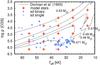 |
Fig. 1 Parameters of studied model stars in Teff vs. log g diagram (red crosses). Overplotted are solar-metallicity evolutionary tracks of Dorman et al. (1993, labelled by a corresponding initial mass) and the positions of single and binary member subdwarfs from Tables 2 and 3. |
The adopted parameters of the model stars are given in Table 1 (effective temperature Teff, radius R∗, and mass M) together with the stellar luminosity L and escape speed vesc. The parameters cover the evolutionary tracks of horizontal branch stars (Dorman et al. 1993) and correspond to the parameters of subdwarfs derived from observations (see Fig. 1). We assumed a canonical mass 0.5 M⊙ for all models. The wind models were calculated for three different metallicities (scalling all elements heavier than helium) Z = 0.1 Z⊙, Z = Z⊙, and Z = 10 Z⊙, where Z is the mass fraction of heavier elements, and Z⊙ = 0.0134 is its solar value. Solar abundances were taken from Asplund et al. (2009).
3. Calculated wind models
We calculated wind models and predicted the basic wind parameters for adopted model stars. The resulting mass-loss rates and terminal velocities are given in Table 1 for individual metallicities. The mass-loss rate can be fitted as 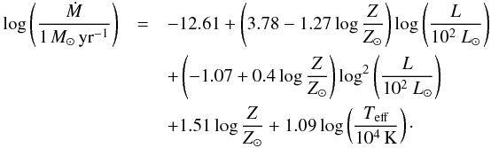 (1)As a result of their high effective temperatures, the mass-loss rate of subdwarf stars is by a factor of about ten higher than the mass-loss rate of main-sequence B stars with the same luminosities (see Fig. 2). The mass-loss rates depend strongly on stellar luminosity and on metallicity. The mass loss varies also with the stellar mass, which is not accounted for in Eq. (1)owing to the fixed stellar mass assumed in our models. Based on findings of Vink & Cassisi (2002), this dependence is expected to be relatively weak.
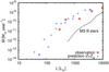 |
Fig. 2 Dependence of the predicted mass-loss rates for Z = Z⊙ (small blue crosses) in comparison with main sequence mass-loss rates of B stars (black line, Krtička 2014) and observed values for subdwarfs from Tables 2 and 3 (large red crosses). The star vZ 1128 is not plotted, since it is a Pop II star with different Z. |
We were unable to calculate converged models for stars with high surface gravities and low effective temperatures. The effect is stronger at low metallicities. These models are denoted as “no wind” in Table 1. The failed convergence of the models indicates that the radiative force is too weak to drive a wind. To test this, we calculated additional models with a fixed hydrodynamical structure, where we compared the radiative force with the gravity for four different fixed mass-loss rates equal to 10-12M⊙ yr-1, 10-13M⊙ yr-1, and 10-14M⊙ yr-1 (for details see Krtička 2014). In all these models, the radiative force was lower than the gravity force. This result supports the conclusion that the radiative force is not able to drive a homogeneous wind and that there is no (hydrogen or helium dominated) wind in the mentioned cases. The position of the stars with no wind is depicted in Fig. 4 by the red shaded area.
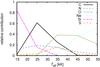 |
Fig. 3 Relative contribution of individual elements to the radiative force at the critical point of the models with Z = Z⊙ as a function of effective temperature. Here we plot the results from models 15-16, 25-08, 35-04, 45-04, and 55-04. |
The winds are driven mainly by the heavier element lines of C, N, O, Ne, and Si (see Fig. 3). The contribution of individual elements varies depending mainly on the effective temperature, but also on the gravity and metallicity. The element whose dominant ionization stage has resonance lines close to the maximum of the flux distribution typically contributes to the radiative force most significantly. The line driving is dominated by Si iv for coolest stars, while more numerous lines of C iii become more significant in hotter stars. The flux with energies higher than that of the Lyman jump becomes significant for line driving in stars with Teff ≈ 35 000 K and, consequently, O iv is important for the wind driving, while numerous lines of Ne v mostly drive the wind in the hottest stars. The plentiful iron lines that are the most efficient wind driver in O stars do not strongly contribute to the radiative force in subdwarfs (Vink & Cassisi 2002). Contrary to less numerous but stronger lines of lighter elements, the iron lines remain optically thin as a result of low iron abundance compared to lighter elements (e.g., Puls et al. 2000; Vink et al. 2001; Krtička 2014). The contribution of iron is only important at the highest metallicity Z = 10 Z⊙.
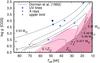 |
Fig. 4 Position of a region with no predicted wind in the Teff vs. log g diagram for two different metallicities (two shades of red regions). Overplotted are the evolutionary tracks of Dorman et al. (1993) and the positions of subdwarf stars with known mass-loss rates derived from observed UV wind-line profiles (blue circles) and X-ray emission (black crosses) – see Tables 2 and 3. Small black dots denote the positions of stars CD-30 11223 (1) and PG1232-136 (2). |
Our models predict a broad range of terminal velocities with the most typical values of about 300−2000 km s-1 depending on stellar parameters (see Table 1). The ratio of the terminal velocity to the escape speed v∞/vesc is typically equal to 1.5−2.5 for solar metallicity subdwafs, which is slightly lower than v∞/vesc = 2.6 found in O stars (Lamers et al. 1995). The terminal velocity clearly scales with metallicity on average as v∞ ~ Z0.2. The metallicity dependence of the terminal velocity and mass-loss rate is stronger than in normal O stars (cf., Krtička 2006).
We calculated additional models with non-solar helium abundance. Helium neither significantly contributes to the radiative force nor affects the emergent flux for subsolar helium abundance. Consequently, our models calculated for N(He) /N(H) = 0.01 showed that the subsolar abundance of helium does not significantly affect the wind mass-loss rate (typically by less than 10%). Our models calculated with enhanced helium abundance (for N(He) /N(H) = 10) showed a slightly higher affect on the mass-loss rate (up to a factor of two) as a result of the influence of helium on the emergent flux.
Subluminous stars show a very wide range of abundances of individual elements. Helium may range from hydrogen-dominated atmospheres with subsolar abundance of helium (e.g., Heber et al. 1999, 2000; Randall et al. 2007; Barlow et al. 2013) to helium dominated atmospheres with only small traces of hydrogen (Thejll et al. 1994; Jeffery & Hamann 2010; Geier et al. 2015). The abundance of heavier elements, which is crucial for the mass-loss rate determination, shows comparable variations from star to star (Husfeld et al. 1989; Jeffery & Hamann 2010; Vos et al. 2013). These abundance differences produce a large diversity of predicted mass-loss rates for individual stars.
4. Comparison with observations and with available theoretical predictions
Parameters of single subluminous stars.
Parameters of individual subluminous stars in binaries.
continued.
We performed a literature search to derive a list of parameters of single subdwarf stars (see Table 2) and subdwarf stars in binaries (see Table 3), including their mass-loss rates derived from UV wind line profiles, the X-ray luminosities LX (preferably in the range 0.2−10 keV, or upper limits), and orbital separation a for binaries. In Tables 2 and 3, we included also the predicted mass-loss rates calculated using Eq. (1), assuming Z = Z⊙. Some stars lie in the region with no wind in the Teff vs. log g diagram (Fig. 4). These stars, for which we do not predict homogeneous winds, are denoted as “no wind” in the Tables. These stars may still have a pure metallic wind, however, with a very low mass-loss rate of the order of 10-16M⊙ yr-1 (Babel 1996).
All listed stars with observed wind line profiles lie outside the region with no predicted winds in the Teff vs. log g diagram in Fig. 4. The X-ray emission of subdwarf stars is presumably connected with their winds. Consequently, stars with X-ray emission should also lie outside the region with no predicted winds. This is also the case for all stars with X-ray emission from our sample, supporting the reliability of our models. In Fig. 2 we compare the predicted dependence of the mass-loss rate on luminosity with available values derived from observations. This comparison shows that the results of our models are also reliable quantitatively.
In binaries consisting of the subdwarf and a compact companion, the X-ray emission may originate from the accretion of the wind on the companion. Consequently, their X-ray luminosity is proportional to the wind mass-loss rate. The upper limit of LX< 1.5 × 1029 erg s-1 in CD-30 11223 thus provides an upper limit for the mass-loss rate Ṁ< 3 × 10-13M⊙ yr-1 (Mereghetti et al. 2014). The estimate of the upper limit of the mass-loss rate Ṁ ≤ 10-13M⊙ yr-1 in PG1232-136 (Mereghetti et al. 2014) is poorly constrained as a result of unknown efficiency for the conversion of accretion power to X-ray luminosity. In any case, both CD-30 11223 and PG1232-136 lie in the region with no winds in Fig. 4. Since only the upper limits of their mass-loss rates are available, this is consistent with our models.
Current models and observations imply that the X-ray emission in O stars originates in their supersonic winds as a result of different processes including instabilities in single stars (Lucy & Solomon 1970; Owocki et al. 1988; Feldmeier et al. 1997), wind collision (e.g., Prilutskii & Usov 1976; Cooke et al. 1978; Pittard 2009), and accretion on compact companion in binaries (Davidson & Ostriker 1973; Lamers et al. 1976). The X-ray luminosity in single O stars and O stars with non-degenerate components is proportional to their stellar luminosity (LX ≈ 10-7L, e.g., Antokhin et al. 2008; Nazé 2009). The origin of this observed relationship is not yet fully understood, but it is possibly connected with the X-ray absorption in the wind (Owocki & Cohen 1999), the density dependence of the radiative cooling (Krtička et al. 2009), and thin-shell mixing in radiative wind-shocks (Owocki et al. 2013). The dependence of the X-ray luminosity on the stellar luminosity in Fig. 5 shows that the detected subdwarf stars follow the extrapolated relation for O stars of Nazé (2009), and also the available upper X-ray detection limits are, in general, in agreement with this relation. Moreover, the observed X-ray luminosities are significantly lower than the wind kinetic energy lost per unit of time  , which indicates that the winds themselves have enough energy to produce the X-rays (Fig. 5).
In Fig. 6 we compare the predicted terminal velocities with values derived from observations as a function of the effective temperature. The terminal velocity is proportional to the escape speed (Puls et al. 2008). In our sample of the stars with winds, the escape speed decreases with effective temperature (like the gravity, see Fig. 4), consequently the terminal velocity also decreases with the effective temperature. This roughly agrees with observations (Fig. 6) taken from Jeffery & Hamann (2010).
The predictions of our models agree with the models of Pauldrach et al. (2004) for central stars of planetary nebulae (Krtička & Kubát 2010a). The predicted mass-loss rates are typically 20% lower than those derived by Krtička & Kubát (2010b). This difference is caused by the line overlaps that were neglected in previous calculations using the Sobolev method. However, our predicted mass-loss rates for subdwarfs are, on average, about one magnitude lower than the predictions of Vink & Cassisi (2002) and Unglaub (2008). The models of Vink & Cassisi (2002) adopt a β-type velocity law and also assume the wind terminal velocity to be equal to the escape speed. Our models consistently calculate the wind velocity from hydrodynamic equations and typically predict a higher terminal velocity, v∞/vesc ≈ 1.5–2.5 (see Table 1). This may significantly affect the predictions, because Vink & Cassisi (2002) use a global energy balance to derive the mass-loss rates. Our tests using the predictions of Vink et al. (2001) showed a factor of 3 difference between the mass-loss rate predictions of O stars calculated for v∞/vesc = 1 and v∞/vesc = 2.5. Solar abundances adopted by Vink & Cassisi (2002) are also higher. Unglaub (2008) neglected the finite disk factor (i.e. he replaced the star with a point source of radiation), which also leads to higher mass-loss rates and lower terminal velocities (Pauldrach et al. 1986; Friend & Abbott 1986). Moreover, the line force multipliers used by Unglaub (2008), which only approximately describe the wind driving force, may lead to larger mass-loss rates. The differences are lower for higher mass-loss rates, which probably reflects a strong decrease of the mass-loss rate close to the wind limit (cf. Krtička 2014).
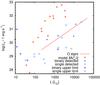 |
Fig. 5 Dependence of X-ray luminosity on the stellar luminosity for subdwarf stars. Individual symbols refer to the X-ray detected binary (filled blue circles) and single (empty blue circles) subdwarf stars and available upper X-ray detection limit in binary (filled blue triangles) and single (empty blue triangles) subdwarf stars from Tables 2 and 3. Overplotted is the extrapolation of the observed mean relation for O stars (Nazé 2009, solid red line) and predicted wind kinetic energy lost per unit of time (for Z = Z⊙, red plus symbols). |
5. The winds of single stars
5.1. Evolutionary implications
Vink & Cassisi (2002) studied the effect of winds on the evolution of subdwarfs and concluded that line driven winds were not strong enough to significantly modify evolutionary tracks for horizontal branch stars and to explain the occurrence of extreme horizontal branch stars in metal-rich clusters. The inspection of the horizontal branch evolutionary tracks of Dorman et al. (1993, see also Schindler et al. 2015) shows that the subdwarfs spend most of their time on a horizontal branch (typically 120−140 Myr) in the region without any wind (for Z ≲ Z⊙, see Fig. 4). Because stars in this part of the Teff vs. log g diagram have typically subsolar chemical composition, they do not lose any mass during a horizontal branch. Such stars have higher effective temperatures or lower gravities after leaving the horizontal branch and they appear in the region with stronger winds in Teff vs. log g diagram. However, a typical duration of this type of evolutionary phase is quite short, typically about 10 Myr (Dorman et al. 1993; Charpinet et al. 2002), consequently the stars lose up to about 0.01 M⊙ of their mass. This is too low to influence the stellar evolution significantly (Vink & Cassisi 2002), but may be enough to strip off a thin hydrogen envelope.
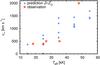 |
Fig. 6 Predicted terminal velocities (blue plus symbols), in comparison with values derived from observations (Jeffery & Hamann 2010, red crosses), as a function of the effective temperature. |
However, some of the objects studied here have larger luminosities and mass-loss rates up to 10-9M⊙ yr-1. Nevertheless, even winds of this greater strength may affect the stellar evolution only if the corresponding evolutionary states last for least 100 Myr. This could possibly be the case of stars with helium-dominated atmospheres. These stars are typically hotter, consequently they may lose a more significant fraction of their mass, provided that the corresponding evolutionary phase is long-lasting.
5.2. Influence of the magnetic field
Magnetic field may strongly influence stellar wind. The effects connected with the magnetic field include modulation of the X-ray flux in magnetospheres filled by the wind (Donati et al. 2002; Nazé et al. 2014), trapping of the wind in corotating magnetosphere (Landstreet & Borra 1978; Townsend et al. 2005), or the rotational braking (ud-Doula et al. 2009). Although there are positive detections of the magnetic field in subdwarf stars, a critical assessment of many of them showed negative results (Landstreet et al. 2012). On the other hand, the available upper limits of the magnetic field intensity in subdwarfs still enable a significant influence of the magnetic field on the wind. This motivates us to study the consequences of magnetic fields in subdwarfs.
The effect of the stellar wind is characterized by the ratio between magnetic field energy density and kinetic energy density of the wind, which may be parameterized by the wind magnetic confinement parameter introduced by ud-Doula & Owocki (2002),  (2)where B is the surface magnetic field strength at the magnetic equator. The larger the magnetic field energy density is, the stronger the influence of the magnetic field on the flow is. The magnetic field significantly affects the wind for η∗ ≳ 1. It follows from Table 1 that for Z = Z⊙ Eq. (2)requires a magnetic field to be as strong as about 100 G to affect the wind in stars with the largest mass-loss rates. Such magnetic fields are comparable with the upper limits of the order of 100 G given in Landstreet et al. (2012). This shows that magnetic fields might be important for the subdwarf winds, even if no field has been confirmed yet.
For η∗> 1 the structure of the flow depends on the relation between the Kepler corotation radius RK = (GM/ Ω2)1 / 3, at which the centrifugal force acting on a corotating matter balances the gravity, and the Alfvén radius RA/R∗ ≈ 0.29 + (η∗ + 0.25)1 / 4 (see ud-Doula et al. 2008; Petit et al. 2013), where the wind kinetic energy density is equal to the magnetic field energy density. Here Ω is the stellar angular frequency of rotation at the stellar surface. The magnetosphere is very dynamic for slowly rotating stars with RA<RK, whereas circumstellar clouds may be generated in stars with centrifugal magnetospheres with RA>RK. Subdwarfs are typically very slowly rotating stars with vrotsini of the order of 1 km s-1 (Geier & Heber 2012), which gives the Kepler corotation radius RK of the order of tens stellar radii. This shows that the case of dynamic magnetospheres is typical in subdwarf stars.
Magnetic subdwarfs with winds lose angular momentum by magnetized winds. The rate of this process may be characterized by the spin-down time,  , where J is the stellar angular momentum. The spin-down time depends on basic stellar parameters, moment of inertia constant k, polar magnetic field strength Bp, and the wind parameters, τspin ~ kM(v∞/Ṁ)1 / 2/ (BpR∗) (ud-Doula et al. 2009, Eq. (25)). To estimate the moment of inertia constant k, we used MESA evolutionary models (Paxton et al. 2011, 2013). We started with He core flash model (with ZAMS mass 1 M⊙ and metallicity Z = 0.02) and applied large mass loss that removes the envelope. The models end up with a subdwarf star with mass 0.46 M⊙. The moment of inertia constant k = 1.2 × 10⁻³ was derived from the moment of inertia of the model.
For stellar parameters corresponding to subdwarfs with the largest mass-loss rates (e.g., BD+37°1977, BD+37°442, and HD 49798, see Tables 2 and 3), and Bp = 100 G, we derive from Eq. (25) of ud-Doula et al. (2009) a spin-down time of the order of 1 Myr. This is shorter than the evolutionary timescale of subdwarf stars (Dorman et al. 1993). The spin-down time is also significantly shorter than for main-sequence B stars as a result of a compact core (and low value of k, cf., Krtička 2014). The spin-down time could be even shorter for stars with a stronger field. Moreover, the magnetic field may be strongly amplified in a merger event (Zhu et al. 2015), which is one formation channel of subdwarf stars. We conclude that magnetic braking can be important in subdwarfs with wind and a magnetic field, and may possibly explain the low rotational velocities observed in these stars (Geier & Heber 2012). A similar effect was proposed by Vink & Cassisi (2002) for non-magnetic stars.
6. The winds of binaries with subdwarf components
6.1. Compact companions: the effect of X-ray irradiation
Several subdwarf stars exist in binaries with compact companions. These binaries are most luminous in the X-ray domain among objects containing subdwarfs. Their X-ray emission originates in the accretion of wind by a compact companion. There is a feedback effect of produced X-rays on the ionization structure of subdwarf stars. We provide wind models that describe this effect of X-ray irradiation. For our study,we selected model 45-08, which has parameters close to known subdwarfs in compact binaries (e.g., BD+37°442, see Table 3).
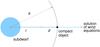 |
Fig. 7 Geometry of the model of a subdwarf wind irradiated by X-rays from a compact companion. |
We studied the effect of X-ray irradiation on the subdwarf wind in a similar way to our earlier wind-irradiation studies (Krtička et al. 2015), i.e., in the direction to the compact companion (see Fig. 7). The influence of X-rays is expected to be the strongest in this direction. Moreover, the accreted wind is assumed to originate from the subdwarf surface that faces the compact companion. The X-ray source coincides with the compact companion in our models. The influence of the X-ray irradiation is taken into account as an additional term in the mean specific intensity, 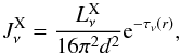 (3)where
  is the luminosity per unit of frequency (we assume
  ), d = | a−r | is the distance to the X-ray source from the point in the wind with radius r (neglecting the radius of a compact companion), the optical depth between a given point and the X-ray source is
 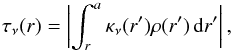 (4)and κν(r′) is the opacity per unit of mass. In our approach, the X-rays directly influence only the ionization equilibrium, while other effects are neglected. We calculate a grid of wind models for different X-ray luminosities
  and different binary separations a.
The radial velocity may become non-monotonic in the presence of the external irradiation. In this case, we cannot calculate the CMF line force directly. However, we calculate the ratio of the CMF and Sobolev line force (see Krtička & Kubát 2010a) for a model without external X-ray irradiation and use this ratio to correct the Sobolev line force in the models with external X-ray irradiation (Krtička et al. 2015). We note that, by taking this approach, we neglect non-local radiative coupling between absorption zones, which occurs in the non-monotonic winds (Rybicki & Hummer 1978; Feldmeier & Nikutta 2006).
To simplify the calculation of  in Eq. (3), we use a density and absorption coefficient in the form of
 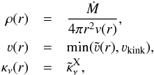 (5)where
  is the depth-independent approximation of X-ray opacity, νkink is equal to the velocity of the kink,if it is present in the models, and otherwise νkink = ∞. The fits to the wind velocity
  and absorption coefficient
  are derived from the model with no external irradiation. The wind velocity is fitted as
 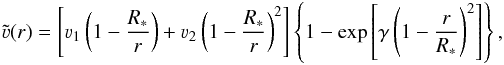 (6)where ν1, ν2, and γ are free parameters of the fit given in Table 4. The polynomial expansion in Eq. (6)provides a better fit of the model wind velocity than a more commonly used β velocity law (Krtička & Kubát 2011). The X-ray opacity per unit of mass averaged for radii 1.5 R∗−5 R∗ is approximated as
 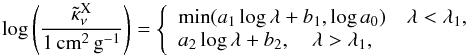 (7)where λ1 = 20.18. The parameter λ is non-dimensional and has the same value as the wavelength in units of Å. Here a0, a1, b1, a2, and b2 are parameters of the fit given in Table 4.
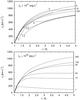 |
Fig. 8 Wind radial velocity as a function of radius in the model 45-08 with external X-ray irradiation (for two different values of the X-ray luminosity LX given in the plots) for Z = Z⊙. Individual curves are indicated by the distance a between the subdwarf and the X-ray source in units of R⊙. |
The calculated models for LX = 1031 erg s-1 and LX = 1035 erg s-1 are given in Fig. 8 for different distances a between the X-ray source and the subdwarf. The presence of an X-ray source causes a shift in the wind ionization towards ions with a higher charge. This affects the radiation force. For a lower amount of X-ray irradiation, new ionization states emerge that are able to drive the wind, and the ionization states with lower charge still remain populated. Consequently, the radiative force increases. However, for stronger X-ray irradiation, the ions with a lower charge disappear, which leads to the decrease of the radiative force. This may even lead to wind inhibition in the direction towards the compact companion (Krtička et al. 2015).
This explains the trends given in Fig. 8 for models with both LX = 1031 erg s-1 and LX = 1035 erg s-1. For a large distance of the X-ray source, the wind is not significantly affected by the X-ray irradiation. For a closer X-ray source, the radiative force increases. Even for a closer X-ray source, the X-ray ionization is so strong that the wind is not able to accelerate efficiently and the kink in the velocity law appears close to the position of the X-ray source (Feldmeier & Shlosman 2000; Feldmeier et al. 2008). If the kink approaches the wind critical point, where the mass-loss rate of our models is determined, the wind driving is significantly suppressed, which leads to wind inhibition. The wind mass flux may be by one or two orders of magnitude lower in the direction of the compact companion. However, we do not model this effect in detail, because this would require time-dependent models.
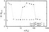 |
Fig. 9 Wind mass-loss rate with X-ray irradiation as a function of the X-ray source distance. The mass-loss rate is plotted relative to the case without any X-ray irradiation for two values of X-ray luminosities. |
A strong increase of the mass-loss rate for the models with a ≈ 2 R⊙ in the case of LX = 1031 erg s-1 and a ≈ 50 R⊙ for LX = 1035 erg s-1 (see Fig. 9) resembles the bistability jump in B supergiants (Pauldrach & Puls 1990; Vink et al. 1999) and has a similar cause. With the increasing influence of X-rays, the radiative force slightly increases in such a way that the density rises and the wind ionization shifts towards ions with a lower charge. The most important is a change of a dominant ionization state of iron from Fe vi to Fe v, but other elements play a role as well. The ionization shift leads to an increase of the radiative force and mass-loss rate. This effect is likely limited to very specific stellar parameters (effective temperature, metallicity) and may not be common among subdwarfs. The range of X-ray source distance a for which the mass-loss rate significantly increases depends on the X-ray luminosity. However, if the curves are plotted as a function of a−R∗, they are similar for different X-ray luminosities.
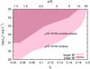 |
Fig. 10 Diagram of the X-ray luminosity LX versus the optical depth parameter tX. The dark red area indicates the region of parameters, where X-rays inhibit the stellar wind, the light red area indicates the region of parameters, where X-rays increase the mass-loss rate, and there is no strong effect of X-rays on the mass-loss rate in the white area. Overplotted is the position of the star HD 49798, corresponding to time period of X-ray eclipse and time period outside the X-ray eclipse (with LX ≈ 1032 erg s-1, Mereghetti et al. 2013). |
The derived results can be summarized in the diagram of the X-ray luminosity versus the optical depth parameter (introduced by Krtička et al. 2015): (8)The optical depth parameter is proportional to the optical depth between the X-ray source and the critical point of the stellar wind (Krtička et al. 2015). For low X-ray luminosities (or large tX, see Fig. 10) the influence of X-rays can be neglected. For higher X-ray luminosities or slightly lower tX the X-ray irradiation strongly affects the wind ionization state, which in a particular case leads to the increase of the wind-mass flux in a direction towards the companion. For even higher X-ray luminosities (lower tX), the X-rays start to disrupt the wind and decrease the wind mass flux. The position of HD 49798 close to the border of the area with lower mass-loss rate indicates that the X-ray emission of this star may be self-regulated, similar to some high-mass X-ray binaries (Krtička et al. 2015). The self-regulated X-ray emission means that a higher X-ray emission may lead to the wind inhibition and therefore to the decrease of LX, whereas a lower X-ray emission leads to an increase of the mass flux and increase of LX. Analogous effects were also predicted in main-sequence star winds (Parkin & Sim 2013; Krtička et al. 2015).
Our models provide just the wind structure in the direction of the compact companion, where the effect of X-rays is the strongest. The influence of X-rays is weaker in other directions forming the photoionization wake (Fransson & Fabian 1980). For a strong X-ray irradiation, this leads to the dependence of the wind-mass flux on the location on the stellar surface. The flow is also influenced by the gravity of the compact object (accretion wake), consequently the numerical simulations are necessary to study this problem in detail (Blondin et al. 1990; Feldmeier et al. 1996; Čechura & Hadrava 2015).
6.2. Late-type main-sequence companions: winds in interaction
Cool main-sequence stars are typical companions of subdwarf stars (see Table 3). These stars may have a solar type (coronal) wind with typical mass-loss rates 10-14−10-11M⊙ yr-1 and terminal velocities of the order of 100 km s-1 that depend on stellar parameters including age (Wood et al. 2005; Holzwarth & Jardine 2007; Cranmer & Saar 2011). Winds of cool companions may interact with the wind of a subdwarf star or accrete on the surface of a subdwarf if the subdwarf wind is either missing or too weak.
The physics of interacting winds is rather complex (e.g., Pittard 2009; Madura & Groh 2012; Parkin et al. 2014). To understand the basic structure of the interaction of a cool wind from a hot star and a hot wind from a cool star, we introduce a simplified picture. We assume that the interaction proceeds through a series of shocks that form a collisional front. Furthermore, we assume that the collisional front is globally in equilibrium, which means that the momenta deposited per unit of time and surface by the wind of both components are equal in magnitude. Consequently, at the intersection of both components (e.g., Mihalas & Mihalas 1999; Antokhin et al. 2004),  (9)where we explicitly included the influence of the cool star wind thermal energy. Here the subscripts sd and MS denote the wind parameters (density ρ, terminal velocity ν, and thermal speed c) of subdwarf star and cool main-sequence star, respectively. We assumed that the winds had already reached the corresponding terminal velocities, and that the subdwarf wind thermal energy can be neglected, since csd ≪ vsd. Denoting the radial distances of the shock front from the individual star centres Dsd and DMS and using the continuity equation, we find
  (10)with a = Dsd + DMS. This equation, in principle, enables us to determine the fate of both winds, but it cannot be used in practice owing to problems with the determination of mass-loss rates and velocities of cool star wind. However, it can at least help us to understand what a typical result of wind collision could be.
For DMS<RMS, the shock position predicted using Eq. (10)would be inside the star. Consequently, the subdwarf wind accretes directly on the cool companion. Within the Bondi-Hoyle-Lyttleton accretion model, the wind is accreted from the radius rHL = 2GMMS/v2, where  (νorbit is orbital velocity). The Bondi-Hoyle-Lyttleton accretion radius corresponds to the radius from which the escape speed is equal to v. Because the speed of the subdwarf wind is typically higher than the escape speed from the main-sequence star, the accretion radius is lower than the stellar radius rHL<RMS. Consequently, we can use the radius of the main-sequence star to calculate the amount of mass accreted per unit of time on the main-sequence star,
  , which follows from geometrical considerations. The mass of cool main-sequence star atmosphere is from the ATLAS model grid (Kurucz 2005; Castelli 2005) of the order of 10-11−10-10M⊙. Since the radius of a cool companion is of the order of 1 R⊙ and the distance is typically also of the same order (see Table 3), the subdwarf star wind replenishes the cool companion atmosphere within the time period of the order of years. Consequently, the chemical composition of the cool companion derived from spectroscopy should be the same as the chemical composition of the subdwarf. This effect was observed in AA Dor (Vučković et al. 2016), for which we predict the existence of a subdwarf wind, and which has a sufficiently low semimajor axis (Table 3). Given a typical lifetime of subdwarf stars of the order of 108 yrs (Dorman et al. 1993), in binaries with extreme mass-loss rate of the order of 10-9M⊙ yr-1, the cool companion may accrete a significant fraction of the subdwarf’s mass. Moreover, the wind is colliding with main-sequence star via a shock, which creates X-rays with X-ray luminosity
  . Because a and RMS are of the same order in many binaries (see Table 3), the X-ray source is comparable to the intrinsic X-ray emission of single subdwarf star (see Fig. 5). Therefore, the X-ray observations of such objects may show orbital modulation. Binary HFG 1 is an ideal test case, because it has a relatively close cool companion and observed X-ray emission (Table 3).
Other cases apart from DMS<RMS are either less common (due to lower mass-loss rate of a main-sequence star wind) or less observationally appealing owing to larger orbital separation. For DMS>RMS and Dsd>Rsd, the two winds collide creating an interacting zone with a complex structure. Such interacting winds are common in hot star wind binaries (e.g. Antokhin et al. 2004; Parkin et al. 2014) and may lead to X-ray variability with orbital period (Nazé et al. 2012). For Dsd<Rsd, the main-sequence star wind collides with the subdwarf star, which leads to similar effects as for DMS<RMS, but affects the subdwarf star.
Cool stars are also X-ray sources with typical X-ray luminosities 1026−1030 erg s-1 (Caillault & Helfand 1985; Drake et al. 1991; Daniel et al. 2002; Schmitt & Liefke 2004). Such X-ray luminosities typically do not influence the subdwarf wind unless the stars are very close. For example, for a model 45-08 this means a ≲ 1.5Rsd for LX ≳ 1029 erg s-1 (see Sect. 6.1). These low orbital separations are not common in subdwarf binaries (see Table 3).
6.3. Be star companions: disk and wind interaction
In some relatively rare cases, the companion of a subdwarf star is a Be star. Be stars are fast rotating non-supergiant stars which have, or had, emission lines owing to an equatorial disk (see Rivinius et al. 2013, for a recent review). The radiation from the subdwarf may interact with the disk of the Be star (e.g., Gies et al. 1998; Koubský et al. 2012, 2014). Moreover, if the subdwarf has a wind (e.g., in ϕ Per or FY CMa, see Table 3), then there is a mechanical interaction between a subdwarf wind and a Be-star disk in the region, where the ram pressures of the Be-star disk and subdwarf wind are equal. Here we shall derive the location of this interaction region.
Because the wind of the subdwarf star is supersonic, the mechanical interaction proceeds via a series of shocks (discontinuities, see Kurfürst et al. 2014). The location of the interaction region in the equatorial plane follows from Eq. (9). The Be-star disks are subsonic to large distances from the Be star (Okazaki 2001; Kurfürst et al. 2014), consequently Eq. (9)can be rewritten as 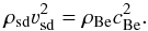 (11)Inserting the midplane disk density (Krtička et al. 2011)
 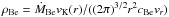 , where
  is the disk orbital (Keplerian) velocity at radius r, and approximating the radial disk velocity vr ≈ cBer/Rcrit with the disk sonic radius
 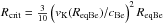 (Krtička et al. 2011), where for a critically rotating star the equatorial radius ReqBe = 3 / 2RBe, we derive from Eq. (11)the equation for the distance r of the interaction region from the Be star
 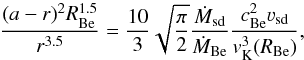 (12)which has to be solved numerically. Here we applied the wind continuity equation Ṁsd = 4π(a−r)2ρsdνsd valid at the distance a−r from subdwarf and identity vK(r) = (RBe/r)1 / 2vK(RBe). We note that a is the distance between centers of both binary components.
For ϕ Per with MBe ≈ 9 M⊙ and RBe ≈ 5 R⊙ (Harmanec 1988, for spectral type from Table 3), cBe ≈ 20 km s-1, Ṁsd = 3 × 10⁻⁹M⊙ yr-1, νsd = 1400 km s-1, we derive for ṀBe = 10-10−10-8M⊙ yr-1 (Granada et al. 2013) the interaction radius r = 0.2a−0.6a = 50−120 R⊙, which corresponds to the size of a Be-star disk of 63 R⊙, which was derived from observations (Quirrenbach et al. 1997; Gies et al. 1998).
7. Discussion
7.1. Inefficient shock radiative cooling
As a result of the dependence of the radiative force on velocity the wind line driving leads to an instability, which subsequently steepens in shocks (Lucy & White 1980; Owocki & Rybicki 1984; Owocki et al. 1988). Since the wind density is relatively high in luminous hot stars, the post-shock material quickly cools down radiatively. Consequently, the bulk of the wind material has a temperature that is comparable to the stellar effective temperature (Feldmeier et al. 1997). Because of the dependence of cooling on the density, the radiative cooling is less effective in weaker winds, and the wind shocks change from radiative to adiabatic (Owocki et al. 2013). This effect may explain weak wind line profiles observed in some low-luminosity O stars (Cohen et al. 2008; Krtička & Kubát 2009; Lucy 2012). In this case, the wind does not cool effectively after the first shock and stays hot. The shocks appear in the highly supersonic part of the wind (Owocki et al. 1988; Feldmeier et al. 1997), consequently the decreasing efficiency of the radiative cooling does not affect the mass-loss rate, but may affect the terminal velocity as a result of the inefficient radiative force.
The problem of inefficient shock radiative cooling has to be addressed with numerical simulations. Krtička & Kubát (2010b) provide an analytical estimate for the ratio of the cooling and hydrodynamic time scales for subdwarf stars. The shock cooling time τs can be estimated as a ratio of the kinetic energy density of post-shock gas and the cooling function, τs ≈ 3 / 2(ρs/mpμ)kTs/ ((ρs/mpμ)2Λ(Ts)), where ρs is the post-shock density, which can be estimated for infinitely strong shocks as ρs = 4ρ = Ṁ/ (πr2v), mp is the mass of the proton, μ is the mean molecular weight, Ts is the post-shock temperature, v is radial wind velocity, and Λs(Ts) is the cooling function (Zel’dovich & Raizer 2002, see also Owocki et al. 2013). The energy conservation for the post-shock velocity vs = v/ 4 requires that the post-shock temperature is Ts = 3μmpv2/ (16k). With the hydrodynamical time-scale τh = r/v the ratio of the shock cooling time to the hydrodynamic time-scale is 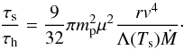 (13)The cooling function has a relatively complex dependence on temperature (Raymond & Smith 1977), and using calculations of Schure et al. (2009) for solar chemical composition (Λ(Ts) ≈ 4.4 × 10⁻²³(Ts/ 107 K)1 / 2 erg cm3 s-1, see Owocki et al. 2013) the ratio Eq. (13)can be cast in numerical form:
 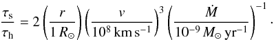 (14)Equation (14)shows that for subdwarfs with the mass-loss rate of the order of 10-9M⊙ yr-1 at a distance of about 1 R⊙, where the wind velocity is of the order of 100 km s-1, the shock cooling time is lower than the hydrodynamic time-scale. Consequently, the shocks are radiative for these stars and do not significantly alter mean wind structure. For subdwarfs with lower wind mass-loss rates (Ṁ ≲ 10-11M⊙ yr-1), a significant part of the wind may not be cooled down efficiently. For these stars, we expect the same mass-loss rate as predicted by our models, but we expect lower terminal velocities and weaker wind line profiles.
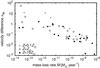 |
Fig. 11 Maximum relative velocity difference between the wind components and hydrogen (Eq. (18) in Krtička 2006) as a function of the wind mass-loss rate for models with different metallicities. |
Besides the radiative cooling, the adiabatic cooling may also affect the post-shock temperature (Zhekov & Skinner 2000; Antokhin et al. 2004). Because the typical cooling length owing to adiabatic cooling is about r (e.g., Owocki et al. 2013), the adiabatic cooling time is roughly equal to the hydrodynamical timescale. Consequently, Eq. (14)also governs the transition from the radiative to the adiabatic shocks.
7.2. Effects connected with multicomponent flow
The line radiative driving mostly impinges on heavier elements in hot star winds (see Fig. 3), while the radiative force on hydrogen and helium is less significant. However, hydrogen and helium constitute the bulk of the wind material, consequently the momentum has be transferred from heavier ions to hydrogen and helium by Coulomb collisions. In dense winds, this process is very effective, consequently the winds can be treated as a one-component flow with equal velocities of all ions (Castor et al. 1976). However, in low-density winds the Coulomb collisions become less efficient, which subsequently leads to the heating of the stellar wind and decoupling of wind components (Springmann & Pauldrach 1992; Owocki & Puls 2002; Krtička 2006; Votruba et al. 2007).
The multicomponent effects can be important in low-density winds of hot subdwarfs (Krtička & Kubát 2010b; Votruba et al. 2010). The importance of the multicomponent effects can be estimated from the value of the relative velocity difference xhp (Eq. (18) in Krtička 2006) between a given element h and protons. For xhp ≲ 0.1, the multicomponent effects are unimportant, for xhp ≳ 0.1 the frictional heating typically influences the wind temperature, and for xhp ≳ 1, the wind components decouple.
We calculated the relative velocity difference xhp according to Krtička (2006) for all considered elements in all models. The relative velocity difference xhp increases with radius as a result of the decreasing density and reaches maximum in the outer parts of the wind, where the radiative acceleration is still significant. We plot the maximum velocity difference between the heavier ions and hydrogen reached in the wind as a function of the mass-loss rate in Fig. 11. The plot is not completely monotonic, because the value of xhp depends also on the wind velocity and temperature (see Eq. (24) in Krtička 2006), and on the charge and mass of heavier ions that mostly drive the wind, which also depend on the stellar parameters.
For high wind mass-loss rates Ṁ ≳ 10-10M⊙ yr-1 the maximum non-dimensional velocity difference is low, xhp< 0.1, and therefore the flow can be treated as a one-component one. For lower wind mass-loss rates 10-12M⊙ yr-1 ≲ Ṁ ≲ 10-10M⊙ yr-1 the maximum non-dimensional velocity difference is higher, 0.1 <xhp< 1, consequently the wind may be frictionally heated. This does not affect the mass-loss rate, but may cause decoupling of the components in the outer wind, because friction decreases with temperature. For low mass-loss rates Ṁ ≲ 10-12M⊙ yr-1 the wind decouples. However, only in the star with the lowest mass-loss rates of about Ṁ ≈ 10-14M⊙ yr-1 does decoupling occur close to the critical point, where the wind velocity is equal to the speed of the Abbott (1980) radiative-acoustic waves. Because the mass-loss rate of our models is determined below this region, decoupling mostly affects the wind terminal velocity and not the mass-loss rate.
Most stars with observed winds have large mass-loss rates Ṁ ≳ 10-10M⊙ yr-1 (see Tables 2 and 3), consequently the multicomponent effects in their winds are expected to be insignificant. Only in the case of the star BD +75°325 the mass-loss rate may be so low that the frictional heating may affect the wind temperature.
8. Conclusions
We calculated wind models suitable for subluminous hot stars. Our models derive level populations from NLTE equations and use hydrodynamical equations with CMF radiative force to predict the wind structure, i.e., the radial dependence of density, velocity, and temperature. Our models therefore predict the basic wind parameters, the mass-loss rate, and the terminal velocity, as a function of stellar parameters, which include stellar effective temperature, mass, radius, and chemical composition.
We tested our derived wind parameters, showing that both the predicted mass-loss rates and terminal velocities agree with values derived from observations. Our models do not predict any winds for stars with low effective temperatures and high surface gravities, while the winds may be strong (Ṁ ≈ 10-10−10-9M⊙ yr-1) for stars with large luminosities. This result is in agreement with the position of stars with and without observed X-ray emission in the log g vs. Teff diagram. We fitted our derived mass-loss rates as a function of the stellar luminosity, effective temperature, and metallicity.
We estimated the impact of the stellar winds on the evolution of subdwarf stars. Stars with high mass-loss rates Ṁ ≳ 10-9M⊙ yr-1 may lose a substantial part of their mass and possibly also angular momentum if they additionally host a magnetic field. The angular momentum loss via magnetized winds may explain low rotational velocities observed in some subdwarf stars.
We studied the winds in binaries that host a subdwarf star. The wind radiative driving in binaries with compact companions may be affected by the presence of a strong X-ray source. The subdwarf winds are accreted on the surface of nearby cool main-sequence companions, which affects their apparent chemical composition. In binaries with a Be-star companion, we predict a mechanical interaction between wind and disk.
Low-density winds may be affected by the so-called weak wind effect, which is probably caused by inefficient shock cooling. We provide a formula that estimates the importance of this effect from basic stellar and wind parameters. Subdwarf winds are prone to this effect for low mass-loss rates Ṁ ≲ 10-11M⊙ yr-1. These weak winds may also show multicomponent structure with the difference between the heavier elements and hydrogen and helium becoming comparable with the thermal speed. Moderate winds trigger some abundance peculiarities, while strong winds wash out any peculiarities (Vauclair 1975; Landstreet et al. 1998; Unglaub 2008; Vick et al. 2011). Consequently, winds in subluminous stars may be also important for the explanation of surface abundances.
The stellar winds constitute an important property of luminous subdwarfs. They may affect their spectra, evolution, and interaction with a potential companion.
Acknowledgments
We thank Drs. S. Mereghetti and P. Németh for discussing the topic. This research was supported by GA ČR 13-10589S. Access to computing and storage facilities owned by parties and projects contributing to the National Grid Infrastructure MetaCentrum, provided under the programme Projects of Large Infrastructure for Research, Development, and Innovations (LM2010005), is greatly appreciated.
References
- Abbott, D. C. 1980, ApJ, 242, 1183 [NASA ADS] [CrossRef] [Google Scholar]
- Afşar, M., & Ibanoǧlu, C. 2008, MNRAS, 391, 802 [NASA ADS] [CrossRef] [Google Scholar]
- Almeida, L. A., Jablonski, F., Tello, J., & Rodrigues, C. V. 2012, MNRAS, 423, 478 [NASA ADS] [CrossRef] [Google Scholar]
- Antokhin, I. I., Owocki, S. P., & Brown, J. C. 2004, ApJ, 611, 434 [NASA ADS] [CrossRef] [Google Scholar]
- Antokhin, I. I., Rauw, G., Vreux, J.-M., van der Hucht, K. A., & Brown, J. C. 2008, A&A, 477, 593 [NASA ADS] [CrossRef] [EDP Sciences] [Google Scholar]
- Asplund, M., Grevesse, N., Sauval, A. J., & Scott, P. 2009, ARA&A, 47, 481 [NASA ADS] [CrossRef] [Google Scholar]
- Aungwerojwit, A., Gänsicke, B. T., Rodríguez-Gil, P., et al. 2007, A&A, 469, 297 [NASA ADS] [CrossRef] [EDP Sciences] [Google Scholar]
- Aznar Cuadrado, R., & Jeffery, C. S. 2002, A&A, 385, 131 [NASA ADS] [CrossRef] [EDP Sciences] [Google Scholar]
- Babel, J. 1996, A&A, 309, 867 [NASA ADS] [Google Scholar]
- Barlow, B. N., Dunlap, B. H., Clemens, J. C., et al. 2010, MNRAS, 403, 324 [NASA ADS] [CrossRef] [Google Scholar]
- Barlow, B. N., Dunlap, B. H., Clemens, J. C., et al. 2011, MNRAS, 414, 3434 [NASA ADS] [CrossRef] [Google Scholar]
- Barlow, B. N., Wade, R. A., & Liss, S. E. 2012a, ApJ, 753, 101 [NASA ADS] [CrossRef] [Google Scholar]
- Barlow, B. N., Wade, R. A., Liss, S. E., Østensen, R. H., & Van Winckel, H. 2012b, ApJ, 758, 58 [NASA ADS] [CrossRef] [Google Scholar]
- Barlow, B. N., Kilkenny, D., Drechsel, H., et al. 2013, MNRAS, 430, 22 [NASA ADS] [CrossRef] [Google Scholar]
- Baschek, B., Scholz, M., Kudritzki, R. P., & Simon, K. P. 1982, A&A, 108, 387 [NASA ADS] [Google Scholar]
- Bauer, F., & Husfeld, D. 1995, A&A, 300, 481 [NASA ADS] [Google Scholar]
- Bisscheroux, B. C., Pols, O. R., Kahabka, P., Belloni, T., & van den Heuvel, E. P. J. 1997, A&A, 317, 815 [NASA ADS] [Google Scholar]
- Bloemen, S., Marsh, T. R., Østensen, R. H., et al. 2011, MNRAS, 410, 1787 [NASA ADS] [Google Scholar]
- Blondin, J. M., Kallman, T. R., Fryxell, B. A., & Taam, R. E. 1990, ApJ, 356, 591 [NASA ADS] [CrossRef] [Google Scholar]
- Budaj, J., Elkin, V., & Hubeny, I. 2003, Modelling of Stellar Atmospheres, 210, 44P [Google Scholar]
- Caillault, J.-P., & Helfand, D. J. 1985, ApJ, 289, 279 [NASA ADS] [CrossRef] [Google Scholar]
- Castelli, F. 2005, Mem. Soc. Astron. It. Suppl., 8, 25 [Google Scholar]
- Castor, J. I., Abbott, D. C., & Klein, R. I. 1976, in Physique des mouvements dans les atmosphères stellaires, eds. R. Cayrel, & M. Sternberg (Paris: CNRS), 363 [Google Scholar]
- Čechura, J., & Hadrava, P. 2015, A&A, 575, A5 [NASA ADS] [CrossRef] [EDP Sciences] [Google Scholar]
- Charpinet, S., Fontaine, G., Brassard, P., & Dorman, B. 2002, ApJS, 140, 469 [NASA ADS] [CrossRef] [EDP Sciences] [Google Scholar]
- Charpinet, S., Fontaine, G., Brassard, P., Green, E. M., & Chayer, P. 2005a, A&A, 437, 575 [NASA ADS] [CrossRef] [EDP Sciences] [Google Scholar]
- Charpinet, S., Fontaine, G., Brassard, P., et al. 2005b, A&A, 443, 251 [NASA ADS] [CrossRef] [EDP Sciences] [Google Scholar]
- Charpinet, S., Silvotti, R., Bonanno, A., et al. 2006, A&A, 459, 565 [NASA ADS] [CrossRef] [EDP Sciences] [Google Scholar]
- Chayer, P., Dixon, W. V., Fullerton, A. W., Ooghe-Tabanou, B., & Reid, I. N. 2015, MNRAS, 452, 2292 [NASA ADS] [CrossRef] [Google Scholar]
- Cohen, D. H., Kuhn, M. A., Gagné, M., Jensen, E. L. N., & Miller, N. A. 2008, MNRAS, 386, 1855 [NASA ADS] [CrossRef] [Google Scholar]
- Cooke, B. A., Fabian, A. C., Pringle, J. E. 1978, Nature, 273, 645 [NASA ADS] [CrossRef] [Google Scholar]
- Cranmer, S. R., & Saar, S. H. 2011, ApJ, 741, 54 [NASA ADS] [CrossRef] [Google Scholar]
- Daniel, K. J., Linsky, J. L., & Gagné, M. 2002, ApJ, 578, 486 [NASA ADS] [CrossRef] [Google Scholar]
- Davidson, K., & Ostriker, J. P. 1973, ApJ, 179, 585 [NASA ADS] [CrossRef] [Google Scholar]
- Deetjen, J. L. 2000, A&A, 360, 281 [NASA ADS] [Google Scholar]
- Donati, J.-F., Babel, J., Harries, T. J., et al. 2002, MNRAS, 333, 55 [NASA ADS] [CrossRef] [MathSciNet] [Google Scholar]
- Dorman, B., Rood, R. T., & O’Connell, R. W. 1993, ApJ, 419, 596 [CrossRef] [Google Scholar]
- Drake, S. A., Linsky, J. L., Judge, P. G., & Elitzur, M. 1991, AJ, 101, 230 [NASA ADS] [CrossRef] [Google Scholar]
- Drechsel, H., Heber, U., Napiwotzki, R., et al. 2001, A&A, 379, 893 [NASA ADS] [CrossRef] [EDP Sciences] [Google Scholar]
- Feldmeier, A., & Nikutta, R. 2006, A&A, 446, 661 [NASA ADS] [CrossRef] [EDP Sciences] [Google Scholar]
- Feldmeier, A., & Shlosman, I. 2000, ApJ, 532, L125 [NASA ADS] [CrossRef] [Google Scholar]
- Feldmeier, A., Anzer, U., Boerner, G., & Nagase, F. 1996, A&A, 311, 793 [NASA ADS] [Google Scholar]
- Feldmeier, A., Puls, J., & Pauldrach, A. W. A. 1997, A&A, 322, 878 [NASA ADS] [Google Scholar]
- Feldmeier, A., Rätzel, D., & Owocki, S. P. 2008, ApJ, 679, 704 [NASA ADS] [CrossRef] [Google Scholar]
- Fontaine, G., Green, E., Charpinet, S., et al. 2014, 6th Meeting on Hot Subdwarf Stars and Related Objects, ASP Conf. Ser., 481, 19 [NASA ADS] [Google Scholar]
- For, B.-Q., Green, E. M., Fontaine, G., et al. 2010, ApJ, 708, 253 [NASA ADS] [CrossRef] [Google Scholar]
- Fransson, C., & Fabian, A. C. 1980, A&A, 87, 102 [NASA ADS] [Google Scholar]
- Friend, D. B., & Abbott, D. C. 1986, ApJ, 311, 701 [NASA ADS] [CrossRef] [Google Scholar]
- Geier, S., & Heber, U. 2012, A&A, 543, A149 [NASA ADS] [CrossRef] [EDP Sciences] [Google Scholar]
- Geier, S., Nesslinger, S., Heber, U., et al. 2007, A&A, 464, 299 [NASA ADS] [CrossRef] [EDP Sciences] [Google Scholar]
- Geier, S., Nesslinger, S., Heber, U., et al. 2008, A&A, 477, L13 [NASA ADS] [CrossRef] [EDP Sciences] [Google Scholar]
- Geier, S., Edelmann, H., Heber, U., & Morales-Rueda, L. 2009, ApJ, 702, L96 [NASA ADS] [CrossRef] [Google Scholar]
- Geier, S., Heber, U., Kupfer, T., & Napiwotzki, R. 2010a, A&A, 515, A37 [NASA ADS] [CrossRef] [EDP Sciences] [Google Scholar]
- Geier, S., Heber, U., Podsiadlowski, P., et al. 2010b, A&A, 519, A25 [NASA ADS] [CrossRef] [EDP Sciences] [Google Scholar]
- Geier, S., Østensen, R. H., Heber, U., et al. 2014, A&A, 562, A95 [NASA ADS] [CrossRef] [EDP Sciences] [Google Scholar]
- Geier, S., Fürst, F., Ziegerer, E., et al. 2015, Science, 347, 1126 [NASA ADS] [CrossRef] [Google Scholar]
- Gies, D. R., Bagnuolo, W. G., Jr., Ferrara, E. C., et al. 1998, ApJ, 493, 440 [NASA ADS] [CrossRef] [Google Scholar]
- Granada, A., Ekström, S., Georgy, C., et al. 2013, A&A, 553, A25 [NASA ADS] [CrossRef] [EDP Sciences] [Google Scholar]
- Green, R. F., Liebert, J., & Wesemael, F. 1984, ApJ, 280, 177 [NASA ADS] [CrossRef] [Google Scholar]
- Gruschinske, J., Hamann, W. R., Kudritzki, R. P., Simon, K. P., & Kaufmann, J. P. 1983, A&A, 121, 85 [NASA ADS] [Google Scholar]
- Hamann, W.-R. 2010, Ap&SS, 329, 151 [NASA ADS] [CrossRef] [Google Scholar]
- Hamann, W.-R., Gruschinske, J., Kudritzki, R. P., & Simon, K. P. 1981, A&A, 104, 249 [NASA ADS] [Google Scholar]
- Han, Z., Podsiadlowski, P., & Lynas-Gray, A. E. 2007, MNRAS, 380, 1098 [NASA ADS] [CrossRef] [Google Scholar]
- Harmanec, P. 1988, Bull. Astron. Inst. Czechosl., 39, 329 [Google Scholar]
- Heber, U., Reid, I. N., & Werner, K. 1999, A&A, 348, L25 [NASA ADS] [Google Scholar]
- Heber, U., Reid, I. N., & Werner, K. 2000, A&A, 363, 198 [NASA ADS] [Google Scholar]
- Heber, U., Drechsel, H., Østensen, R., et al. 2004, A&A, 420, 251 [NASA ADS] [CrossRef] [EDP Sciences] [Google Scholar]
- Hilditch, R. W., Harries, T. J., & Hill, G. 1996, MNRAS, 279, 1380 [NASA ADS] [Google Scholar]
- Hirsch H. 2009, Ph.D. Thesis, University of Erlangen-Nürnberg [Google Scholar]
- Holzwarth, V., & Jardine, M. 2007, A&A, 463, 11 [NASA ADS] [CrossRef] [EDP Sciences] [Google Scholar]
- Howarth, I. D., & Heber, U. 1990, PASP, 102, 912 [NASA ADS] [CrossRef] [Google Scholar]
- Hummer, D. G., Berrington, K. A., Eissner, W., et al. 1993, A&A, 279, 298 [NASA ADS] [Google Scholar]
- Husfeld, D., Butler, K., Heber, U., & Drilling, J. S. 1989, A&A, 222, 150 [NASA ADS] [Google Scholar]
- İbanoǧlu, C., Çakırlı, Ö., Taş, G., & Evren, S. 2004, A&A, 414, 1043 [NASA ADS] [CrossRef] [EDP Sciences] [Google Scholar]
- Iben, I., Jr., & Tutukov, A. V. 1984, ApJS, 54, 335 [NASA ADS] [CrossRef] [Google Scholar]
- Iben, I., Jr., Kaler, J. B., Truran, J. W., & Renzini, A. 1983, ApJ, 264, 605 [NASA ADS] [CrossRef] [Google Scholar]
- Jeffery, C. S., & Hamann, W.-R. 2010, MNRAS, 404, 1698 [NASA ADS] [Google Scholar]
- Jeffery, C. S., Ahmad, A., Naslim, N., & Kerzendorf, W. 2015, MNRAS, 446, 1889 [NASA ADS] [CrossRef] [Google Scholar]
- Koen, C., Orosz, J. A., & Wade, R. A. 1998, MNRAS, 300, 695 [NASA ADS] [CrossRef] [Google Scholar]
- Koubský, P., Kotková, L., Votruba, V., Šlechta, M., & Dvořáková, Š. 2012, A&A, 545, A121 [NASA ADS] [CrossRef] [EDP Sciences] [Google Scholar]
- Koubský, P., Kotková, L., Kraus, M., et al. 2014, A&A, 567, A57 [NASA ADS] [CrossRef] [EDP Sciences] [Google Scholar]
- Krtička, J. 2006, MNRAS, 367, 1282 [NASA ADS] [CrossRef] [Google Scholar]
- Krtička, J. 2014, A&A, 564, A70 [Google Scholar]
- Krtička, J., & Kubát, J. 2009, MNRAS, 394, 2065 [NASA ADS] [CrossRef] [Google Scholar]
- Krtička, J., & Kubát, J. 2010a, A&A, 519, A5 [NASA ADS] [CrossRef] [EDP Sciences] [Google Scholar]
- Krtička, J., & Kubát, J. 2010b, Ap&SS, 329, 145 [NASA ADS] [CrossRef] [Google Scholar]
- Krtička, J., & Kubát, J. 2011, A&A, 534, A97 [NASA ADS] [CrossRef] [EDP Sciences] [Google Scholar]
- Krtička, J., Feldmeier, A., Oskinova, L. M., Kubát, J., & Hamann, W.-R. 2009, A&A, 508, 841 [NASA ADS] [CrossRef] [EDP Sciences] [Google Scholar]
- Krtička, J., Owocki, S. P., & Meynet, G. 2011, A&A, 527, A84 [NASA ADS] [CrossRef] [EDP Sciences] [Google Scholar]
- Krtička, J., Kubát, J., & Krtičková, I. 2015, A&A, 579, A111 [NASA ADS] [CrossRef] [EDP Sciences] [Google Scholar]
- Kubát J. 2003, in Modelling of Stellar Atmospheres, eds. N. E. Piskunov, W. W. Weiss, & D. F. Gray, (San Francisco ASP), IAU Symp. 210, A8 [Google Scholar]
- Kubát, J., Puls, J., & Pauldrach, A. W. A. 1999, A&A, 341, 587 [NASA ADS] [Google Scholar]
- Kudritzki, R. P., & Simon, K. P. 1978, A&A, 70, 653 [NASA ADS] [Google Scholar]
- Kupfer, T., Geier, S., Heber, U., et al. 2015, A&A, 576, A44 [NASA ADS] [CrossRef] [EDP Sciences] [Google Scholar]
- Kupka, F., Piskunov, N. E., Ryabchikova, T. A., Stempels, H. C., & Weiss, W. W. 1999, A&AS, 138, 119 [NASA ADS] [CrossRef] [EDP Sciences] [MathSciNet] [PubMed] [Google Scholar]
- Kurfürst, P., Feldmeier, A., & Krtička, J. 2014, A&A, 569, A23 [NASA ADS] [CrossRef] [EDP Sciences] [Google Scholar]
- Kurucz, R. L. 2005, Mem. Soc. Astron. It. Suppl., 8, 1 [Google Scholar]
- Lamers, H. J. G. L. M., van den Heuvel, E. P. J., & Petterson, J. A. 1976, A&A, 49, 327 [NASA ADS] [Google Scholar]
- Lamers, H. J. G. L. M., Snow, T. P., & Lindholm, D. M. 1995, ApJ, 455, 269 [NASA ADS] [CrossRef] [Google Scholar]
- Landstreet, J. D., & Borra, E. F. 1978, ApJ, 224, L5 [NASA ADS] [CrossRef] [Google Scholar]
- Landstreet, J. D., Dolez, N., & Vauclair, S. 1998, A&A, 333, 977 [NASA ADS] [Google Scholar]
- Landstreet, J. D., Bagnulo, S., Fossati, L., Jordan, S., & O’Toole, S. J. 2012, A&A, 541, A100 [NASA ADS] [CrossRef] [EDP Sciences] [Google Scholar]
- Lanz, T., & Hubeny, I. 2003, ApJS, 146, 417 [NASA ADS] [CrossRef] [Google Scholar]
- Lanz, T., & Hubeny, I. 2007, ApJS, 169, 83 [CrossRef] [Google Scholar]
- Lanz, T., Hubeny, I., & Heap, S. R. 1997, ApJ, 485, 843 [NASA ADS] [CrossRef] [Google Scholar]
- Lanz, T., Brown, T. M., Sweigart, A. V., Hubeny, I., & Landsman, W. B. 2004, ApJ, 602, 342 [NASA ADS] [CrossRef] [Google Scholar]
- La Palombara, N., Mereghetti, S., Tiengo, A., & Esposito, P. 2012, ApJ, 750, L34 [NASA ADS] [CrossRef] [Google Scholar]
- La Palombara, N., Esposito, P., Mereghetti, S., & Tiengo, A. 2014, A&A, 566, A4 [NASA ADS] [CrossRef] [EDP Sciences] [Google Scholar]
- La Palombara, N., Esposito, P., Mereghetti, S., Novara, G., & Tiengo, A. 2015, A&A, 580, A56 [NASA ADS] [CrossRef] [EDP Sciences] [Google Scholar]
- Latour, M., Fontaine, G., Chayer, P., & Brassard, P. 2013, ApJ, 773, 84 [NASA ADS] [CrossRef] [Google Scholar]
- Latour, M., Fontaine, G., Green, E. M., Brassard, P., & Chayer, P. 2014, ApJ, 788, 65 [NASA ADS] [CrossRef] [Google Scholar]
- Lucy, L. B., 2012, A&A, 544, A120 [NASA ADS] [CrossRef] [EDP Sciences] [Google Scholar]
- Lucy, L. B., & Solomon, P. M. 1970, ApJ, 159, 879 [NASA ADS] [CrossRef] [Google Scholar]
- Lucy, L. B., & White, R. L. 1980, ApJ, 241, 300 [NASA ADS] [CrossRef] [Google Scholar]
- Madura, T. I., & Groh, J. H. 2012, ApJ, 746, L18 [NASA ADS] [CrossRef] [Google Scholar]
- Maxted, P. F. L., Marsh, T. R., & North, R. C. 2000, MNRAS, 317, L41 [NASA ADS] [CrossRef] [Google Scholar]
- Maxted, P. F. L., Marsh, T. R., Heber, U., et al. 2002, MNRAS, 333, 231 [NASA ADS] [CrossRef] [Google Scholar]
- Mereghetti, S., Campana, S., Esposito, P., La Palombara, N., & Tiengo, A. 2011, A&A, 536, A69 [NASA ADS] [CrossRef] [EDP Sciences] [Google Scholar]
- Mereghetti, S., La Palombara, N., Tiengo, A., et al. 2013, A&A, 553, A46 [NASA ADS] [CrossRef] [EDP Sciences] [Google Scholar]
- Mereghetti, S., La Palombara, N., Esposito, P., et al. 2014, MNRAS, 441, 2684 [NASA ADS] [CrossRef] [Google Scholar]
- Mereghetti, S., Pintore, F., Esposito, P., et al. 2016, MNRAS, submitted [Google Scholar]
- Mihalas, D., & Mihalas, B. 1999, Foundations of Radiation Hydrodynamics (New York: Dower) [Google Scholar]
- Mihalas, D., Kunasz, P. B., & Hummer, D. G. 1975, ApJ, 202, 465 [NASA ADS] [CrossRef] [Google Scholar]
- Miller Bertolami, M. M., & Althaus, L. G. 2006, A&A, 454, 845 [NASA ADS] [CrossRef] [EDP Sciences] [Google Scholar]
- Montez, R., Jr., De Marco, O., Kastner, J. H., & Chu, Y.-H. 2010, ApJ, 721, 1820 [NASA ADS] [CrossRef] [Google Scholar]
- Napiwotzki, R. 1999, A&A, 350, 101 [Google Scholar]
- Naslim, N., Jeffery, C. S., Ahmad, A., Behara, N. T., & Şahìn, T. 2010, MNRAS, 409, 582 [NASA ADS] [CrossRef] [Google Scholar]
- Naslim, N., Jeffery, C. S., Behara, N. T., & Hibbert, A. 2011, MNRAS, 412, 363 [NASA ADS] [CrossRef] [Google Scholar]
- Nazé, Y. 2009, A&A, 506, 1055 [NASA ADS] [CrossRef] [EDP Sciences] [Google Scholar]
- Nazé, Y., Mahy, L., Damerdji, Y., et al. 2012, A&A, 546, A37 [NASA ADS] [CrossRef] [EDP Sciences] [Google Scholar]
- Nazé, Y., Petit, V., Rinbrand, M., et al. 2014, ApJS, 215, 10 [NASA ADS] [CrossRef] [Google Scholar]
- Okazaki, A. T. 2001, PASJ, 53, 119 [NASA ADS] [CrossRef] [Google Scholar]
- Orosz, J. A., & Wade, R. A. 1999, MNRAS, 310, 773 [NASA ADS] [CrossRef] [Google Scholar]
- Østensen, R. H. 2006, Balt. Astron., 15, 85 [NASA ADS] [Google Scholar]
- Østensen, R. H., Oreiro, R., Hu, H., Drechsel, H., & Heber, U. 2008, Hot Subdwarf Stars and Related Objects, 392, 221 [Google Scholar]
- Østensen, R. H., Green, E. M., Bloemen, S., et al. 2010, MNRAS, 408, L51 [NASA ADS] [CrossRef] [Google Scholar]
- Owocki, S. P., & Cohen, D. H. 1999, ApJ, 520, 833 [NASA ADS] [CrossRef] [Google Scholar]
- Owocki, S. P., & Puls, J. 2002, ApJ, 568, 965 [NASA ADS] [CrossRef] [Google Scholar]
- Owocki, S. P., & Rybicki, G. B. 1984, ApJ, 284, 33 [Google Scholar]
- Owocki, S. P., Castor, J. I., & Rybicki, G. B. 1988, ApJ, 335, 914 [NASA ADS] [CrossRef] [Google Scholar]
- Owocki, S. P., Sundqvist, J. O., Cohen, D. H., & Gayley, K. G. 2013, MNRAS, 429, 3379 [NASA ADS] [CrossRef] [Google Scholar]
- Parkin, E. R., & Sim, S. A. 2013, ApJ, 767, 114 [NASA ADS] [CrossRef] [Google Scholar]
- Parkin, E. R., Pittard, J. M., Nazé, Y., & Blomme, R. 2014, A&A, 570, A10 [NASA ADS] [CrossRef] [EDP Sciences] [Google Scholar]
- Pauldrach, A. W. A., & Puls, J. 1990, A&A, 237, 409 [NASA ADS] [Google Scholar]
- Pauldrach, A., Puls, J., & Kudritzki, R. P. 1986, A&A, 164, 86 [NASA ADS] [Google Scholar]
- Pauldrach, A. W. A., Hoffmann, T. L., & Lennon, M. 2001, A&A, 375, 161 [NASA ADS] [CrossRef] [EDP Sciences] [Google Scholar]
- Pauldrach, A. W. A., Hoffmann, T. L., & Méndez, R. H. 2004, A&A, 419, 1111 [NASA ADS] [CrossRef] [EDP Sciences] [Google Scholar]
- Paxton, B., Bildsten, L., Dotter, A., et al. 2011, ApJS, 192, 3 [Google Scholar]
- Paxton, B., Cantiello, M., Arras, P., et al. 2013, ApJS, 208, 4 [NASA ADS] [CrossRef] [Google Scholar]
- Peters, G. J., Gies, D. R., Grundstrom, E. D., & McSwain, M. V. 2008, ApJ, 686, 1280 [Google Scholar]
- Peters, G. J., Pewett, T. D., Gies, D. R., Touhami, Y. N., & Grundstrom, E. D. 2013, ApJ, 765, 2 [NASA ADS] [CrossRef] [Google Scholar]
- Petit, V., Owocki, S. P., Wade, G. A., et al. 2013, MNRAS, 429, 398 [NASA ADS] [CrossRef] [Google Scholar]
- Piskunov, N. E., Kupka, F., Ryabchikova, T. A., Weiss, W. W., & Jeffery, C. S. 1995, A&AS, 112, 525 [NASA ADS] [Google Scholar]
- Pittard, J. M. 2009, MNRAS, 396, 1743 [NASA ADS] [CrossRef] [Google Scholar]
- Prilutskii, O. F., & Usov, V. V. 1976, AZh, 53, 6 [NASA ADS] [Google Scholar]
- Przybilla, N., Butler, K., Heber, U., & Jeffery, C. S. 2005, A&A, 443, L25 [NASA ADS] [CrossRef] [EDP Sciences] [Google Scholar]
- Puls, J., Springmann, U., & Lennon, M. 2000, A&AS, 141, 23 [NASA ADS] [CrossRef] [EDP Sciences] [Google Scholar]
- Puls, J., Vink, J. S., & Najarro, F. 2008, A&ARv, 16, 209 [NASA ADS] [CrossRef] [EDP Sciences] [Google Scholar]
- Quirrenbach, A., Bjorkman, K. S., Bjorkman, J. E., et al. 1997, ApJ, 479, 477 [NASA ADS] [CrossRef] [Google Scholar]
- Randall, S. K., Green, E. M., Van Grootel, V., et al. 2007, A&A, 476, 1317 [NASA ADS] [CrossRef] [EDP Sciences] [Google Scholar]
- Randall, S. K., Van Grootel, V., Fontaine, G., Charpinet, S., & Brassard, P. 2009, A&A, 507, 911 [NASA ADS] [CrossRef] [EDP Sciences] [Google Scholar]
- Rauch, T. 1993, A&A, 276, 171 [NASA ADS] [Google Scholar]
- Rauch, T. 2000, A&A, 356, 665 [NASA ADS] [Google Scholar]
- Rauch, T., & Werner, K. 2003, A&A, 400, 271 [NASA ADS] [CrossRef] [EDP Sciences] [Google Scholar]
- Rauch, T., Rudkowski, A., Kampka, D., et al. 2014, A&A, 566, A3 [NASA ADS] [CrossRef] [EDP Sciences] [Google Scholar]
- Raymond, J. C., & Smith, B. W. 1977, ApJS, 35, 419 [NASA ADS] [CrossRef] [Google Scholar]
- Ribeiro, T., & Baptista, R. 2011, A&A, 526, A150 [NASA ADS] [CrossRef] [EDP Sciences] [Google Scholar]
- Rivinius, T., Carciofi, A. C., & Martayan, C. 2013, A&ARv, 21, 69 [Google Scholar]
- Rodríguez-López, C., Ulla, A., & Garrido, R. 2007, MNRAS, 379, 1123 [NASA ADS] [CrossRef] [Google Scholar]
- Rybicki, G. B., & Hummer, D. G. 1978, ApJ, 219, 645 [Google Scholar]
- Saffer, R. A., Bergeron, P., Koester, D., & Liebert, J. 1994, ApJ, 432, 351 [NASA ADS] [CrossRef] [Google Scholar]
- Saio, H., & Jeffery, C. S. 2000, MNRAS, 313, 671 [NASA ADS] [CrossRef] [Google Scholar]
- Schaffenroth, V., Geier, S., Heber, U., et al. 2011, AIP Conf. Ser., 1331, 174 [Google Scholar]
- Schaffenroth, V., Geier, S., Drechsel, H., et al. 2013, A&A, 553, A18 [NASA ADS] [CrossRef] [EDP Sciences] [Google Scholar]
- Schaffenroth, V., Geier, S., Heber, U., et al. 2014, A&A, 564, A98 [NASA ADS] [CrossRef] [EDP Sciences] [Google Scholar]
- Schaffenroth, V., Barlow, B. N., Drechsel, H., & Dunlap, B. H. 2015, A&A, 576, A123 [NASA ADS] [CrossRef] [EDP Sciences] [Google Scholar]
- Schindler, J.-T., Green, E. M., & Arnett, W. D. 2015, ApJ, 806, 178 [NASA ADS] [CrossRef] [Google Scholar]
- Schmitt, J. H. M. M., & Liefke, C. 2004, A&A, 417, 651 [NASA ADS] [CrossRef] [EDP Sciences] [Google Scholar]
- Schonberner, D., & Drilling, J. S. 1984, ApJ, 278, 702 [NASA ADS] [CrossRef] [Google Scholar]
- Schure, K. M., Kosenko, D., Kaastra, J. S., Keppens, R., & Vink, J. 2009, A&A, 508, 751 [NASA ADS] [CrossRef] [EDP Sciences] [Google Scholar]
- Seaton, M. J., Zeippen, C. J., Tully, J. A., et al. 1992, Rev. Mex. Astron. Astrofis., 23, 19 [NASA ADS] [EDP Sciences] [Google Scholar]
- Shimanskii, V. V., Borisov, N. V., Sakhibullin, N. A., & Surkov, A. E. 2004, Astron. Rep., 48, 563 [NASA ADS] [CrossRef] [Google Scholar]
- Springmann, U. W. E., & Pauldrach, A. W. A. 1992, A&A, 262, 515 [NASA ADS] [Google Scholar]
- Telting, J. H., Østensen, R. H., Baran, A. S., et al. 2012, A&A, 544, A1 [NASA ADS] [CrossRef] [EDP Sciences] [Google Scholar]
- Theissen, A., Moehler, S., Heber, U., Schmidt, J. H. K., & de Boer, K. S. 1995, A&A, 298, 577 [NASA ADS] [Google Scholar]
- Thejll, P., Bauer, F., Saffer, R., et al. 1994, ApJ, 433, 819 [NASA ADS] [CrossRef] [Google Scholar]
- Thejll, P., Ulla, A., & MacDonald, J. 1995, A&A, 303, 773 [Google Scholar]
- Townsend, R. H. D., Owocki, S. P., & Groote, D. 2005, ApJ, 630, L81 [NASA ADS] [CrossRef] [Google Scholar]
- ud-Doula, A., & Owocki, S. P. 2002, ApJ, 576, 413 [NASA ADS] [CrossRef] [Google Scholar]
- ud-Doula, A., Owocki, S. P., & Townsend, R. H. D. 2008, MNRAS, 385, 97 [NASA ADS] [CrossRef] [Google Scholar]
- ud-Doula, A., Owocki, S. P., & Townsend, R. H. D. 2009, MNRAS, 392, 1022 [NASA ADS] [CrossRef] [Google Scholar]
- Ulla, A., & Thejll, P. 1998, A&AS, 132, 1 [NASA ADS] [CrossRef] [EDP Sciences] [Google Scholar]
- Unglaub, K. 2008, A&A, 486, 923 [NASA ADS] [CrossRef] [EDP Sciences] [Google Scholar]
- Vauclair, S. 1975, A&A, 45, 233 [NASA ADS] [Google Scholar]
- Van Grootel, V., Charpinet, S., Fontaine, G., et al. 2010, ApJ, 718, L97 [NASA ADS] [CrossRef] [EDP Sciences] [Google Scholar]
- Van Grootel, V., Charpinet, S., Brassard, P., Fontaine, G., & Green, E. M. 2013, A&A, 553, A97 [NASA ADS] [CrossRef] [EDP Sciences] [Google Scholar]
- Vennes, S., Kawka, A., & Smith, J. A. 2007, ApJ, 668, L59 [NASA ADS] [CrossRef] [Google Scholar]
- Vick, M., Michaud, G., Richer, J., & Richard, O. 2011, A&A, 526, A37 [NASA ADS] [CrossRef] [EDP Sciences] [Google Scholar]
- Vink, J. S., & Cassisi, S. 2002, A&A, 392, 553 [NASA ADS] [CrossRef] [EDP Sciences] [Google Scholar]
- Vink, J. S., de Koter, A., & Lamers, H. J. G. L. M. 1999, A&A, 350, 181 [NASA ADS] [Google Scholar]
- Vink, J. S., de Koter, A., & Lamers, H. J. G. L. M. 2001, A&A, 369, 574 [NASA ADS] [CrossRef] [EDP Sciences] [Google Scholar]
- Viton, M., Burgarella, D., Cassatella, A., & Prevot, L. 1988, A&A, 205, 147 [NASA ADS] [Google Scholar]
- Vos, J., Østensen, R. H., Degroote, P., et al. 2012, A&A, 548, A6 [NASA ADS] [CrossRef] [EDP Sciences] [Google Scholar]
- Vos, J., Østensen, R. H., Németh, P., et al. 2013, A&A, 559, A54 [NASA ADS] [CrossRef] [EDP Sciences] [Google Scholar]
- Votruba, V., Feldmeier, A., Kubát, J., & Rätzel, D. 2007, A&A, 474, 549 [NASA ADS] [CrossRef] [EDP Sciences] [Google Scholar]
- Votruba, V., Feldmeier, A., Krtička, J., & Kubát, J. 2010, Ap&SS, 329, 159 [NASA ADS] [CrossRef] [Google Scholar]
- Vučković, M., Aerts, C., Östensen, R., et al. 2007, A&A, 471, 605 [NASA ADS] [CrossRef] [EDP Sciences] [Google Scholar]
- Vučković, M., Østensen, R. H., Németh, P., Bloemen, S., & Pápics, P. I. 2016, A&A, 586, A146 [NASA ADS] [CrossRef] [EDP Sciences] [Google Scholar]
- Wood, B. E., Müller, H.-R., Zank, G. P., Linsky, J. L., & Redfield, S. 2005, ApJ, 628, L143 [Google Scholar]
- Zel’dovich, Y. B., & Raizer, Y. P. 2002, Physics of Shock Waves and High-temperature Hydrodynamic Phenomena (New York: Dover) [Google Scholar]
- Zhang, X., & Jeffery, C. S. 2012, MNRAS, 419, 452 [NASA ADS] [CrossRef] [Google Scholar]
- Zhekov, S. A., & Skinner, S. L. 2000, ApJ, 538, 808 [NASA ADS] [CrossRef] [Google Scholar]
- Zhou, A.-Y., Reed, M. D., Harms, S., et al. 2006, MNRAS, 367, 179 [NASA ADS] [CrossRef] [Google Scholar]
- Zhu, C., Pakmor, R., van Kerkwijk, M. H., & Chang, P. 2015, ApJ, 806, L1 [NASA ADS] [CrossRef] [Google Scholar]
All Tables
Adopted stellar parameters of the model grid and predicted wind parameters for individual metallicities.
All Figures
|
Fig. 1 Parameters of studied model stars in Teff vs. log g diagram (red crosses). Overplotted are solar-metallicity evolutionary tracks of Dorman et al. (1993, labelled by a corresponding initial mass) and the positions of single and binary member subdwarfs from Tables 2 and 3. |
| In the text | |
|
Fig. 2 Dependence of the predicted mass-loss rates for Z = Z⊙ (small blue crosses) in comparison with main sequence mass-loss rates of B stars (black line, Krtička 2014) and observed values for subdwarfs from Tables 2 and 3 (large red crosses). The star vZ 1128 is not plotted, since it is a Pop II star with different Z. |
| In the text | |
|
Fig. 3 Relative contribution of individual elements to the radiative force at the critical point of the models with Z = Z⊙ as a function of effective temperature. Here we plot the results from models 15-16, 25-08, 35-04, 45-04, and 55-04. |
| In the text | |
|
Fig. 4 Position of a region with no predicted wind in the Teff vs. log g diagram for two different metallicities (two shades of red regions). Overplotted are the evolutionary tracks of Dorman et al. (1993) and the positions of subdwarf stars with known mass-loss rates derived from observed UV wind-line profiles (blue circles) and X-ray emission (black crosses) – see Tables 2 and 3. Small black dots denote the positions of stars CD-30 11223 (1) and PG1232-136 (2). |
| In the text | |
|
Fig. 5 Dependence of X-ray luminosity on the stellar luminosity for subdwarf stars. Individual symbols refer to the X-ray detected binary (filled blue circles) and single (empty blue circles) subdwarf stars and available upper X-ray detection limit in binary (filled blue triangles) and single (empty blue triangles) subdwarf stars from Tables 2 and 3. Overplotted is the extrapolation of the observed mean relation for O stars (Nazé 2009, solid red line) and predicted wind kinetic energy lost per unit of time (for Z = Z⊙, red plus symbols). |
| In the text | |
|
Fig. 6 Predicted terminal velocities (blue plus symbols), in comparison with values derived from observations (Jeffery & Hamann 2010, red crosses), as a function of the effective temperature. |
| In the text | |
|
Fig. 7 Geometry of the model of a subdwarf wind irradiated by X-rays from a compact companion. |
| In the text | |
|
Fig. 8 Wind radial velocity as a function of radius in the model 45-08 with external X-ray irradiation (for two different values of the X-ray luminosity LX given in the plots) for Z = Z⊙. Individual curves are indicated by the distance a between the subdwarf and the X-ray source in units of R⊙. |
| In the text | |
|
Fig. 9 Wind mass-loss rate with X-ray irradiation as a function of the X-ray source distance. The mass-loss rate is plotted relative to the case without any X-ray irradiation for two values of X-ray luminosities. |
| In the text | |
|
Fig. 10 Diagram of the X-ray luminosity LX versus the optical depth parameter tX. The dark red area indicates the region of parameters, where X-rays inhibit the stellar wind, the light red area indicates the region of parameters, where X-rays increase the mass-loss rate, and there is no strong effect of X-rays on the mass-loss rate in the white area. Overplotted is the position of the star HD 49798, corresponding to time period of X-ray eclipse and time period outside the X-ray eclipse (with LX ≈ 1032 erg s-1, Mereghetti et al. 2013). |
| In the text | |
|
Fig. 11 Maximum relative velocity difference between the wind components and hydrogen (Eq. (18) in Krtička 2006) as a function of the wind mass-loss rate for models with different metallicities. |
| In the text | |
Current usage metrics show cumulative count of Article Views (full-text article views including HTML views, PDF and ePub downloads, according to the available data) and Abstracts Views on Vision4Press platform.
Data correspond to usage on the plateform after 2015. The current usage metrics is available 48-96 hours after online publication and is updated daily on week days.
Initial download of the metrics may take a while.