| Issue |
A&A
Volume 593, September 2016
|
|
|---|---|---|
| Article Number | A51 | |
| Number of page(s) | 31 | |
| Section | Interstellar and circumstellar matter | |
| DOI | https://doi.org/10.1051/0004-6361/201628329 | |
| Published online | 19 September 2016 | |
Incidence of debris discs around FGK stars in the solar neighbourhood⋆
1 Departmento de
Astrofísica, Centro de Astrobiología
(CAB, CSIC-INTA), ESAC Campus, Camino Bajo del Castillo s/n, 28692 Villanueva de la
Cañada, Madrid, Spain
e-mail: This email address is being protected from spambots. You need JavaScript enabled to view it.
2 Universidad Autónoma de Madrid, Dpto.
Física Teórica, Módulo 15, Facultad de Ciencias, Campus de Cantoblanco, 28049
Madrid,
Spain
3 Unidad Asociada CAB–UAM
4 Astrophysikalisches Institut und
Universitätssternwarte, Friedrich-Schiller-Universität, Schillergäßchen 2−3,
07745
Jena,
Germany
5 School of Physics,
UNSW Australia, NSW
2052
Sydney,
Australia
6 Australian Centre for Astrobiology,
UNSW Australia, NSW , 2052
Sydney,
Australia
7 ESA, Directorate of Science,
Scientific Support Office, European Space Research and Technology Centre
(ESTEC/SCI-S), Keplerlaan 1, 2201
AZ
Noordwijk, The
Netherlands
8 Department of Earth and Space
Sciences, Chalmers University of Technology, Onsala Space Observatory,
439 92
Onsala,
Sweden
9 ESA-ESAC Gaia SOC, PO Box 78, 28691
Villanueva de la Cañada, Madrid, Spain
10 INAF, Osservatorio Astronomico di
Palermo, Piazza Parlamento 1, 90134
Palermo,
Italy
11 Institute of Theoretical Physics
and Astrophysics, Christian-Albrechts University Kiel, Leibnizstr. 15, 24118
Kiel,
Germany
12 Steward Observatory, Department of
Astronomy, University of Arizona, 933 North Cherry Avenue, Tucson, AZ
85721,
USA
13 Instituto de Física y Astronomía,
Facultad de Ciencias, Universidad de Valparaíso, Av. Gran Bretaña 1111, 5030 Casilla,
Valparaíso,
Chile
14 ICM Nucleus on Protoplanetary
Disks, Universidad de Valparaíso, Av. Gran Bretaña 1111, 2360102
Valparaíso,
Chile
15 Univ. Grenoble Alpes, IPAG,
38000
Grenoble,
France
16 CNRS, IPAG, 38000
Grenoble,
France
17 Leiden Observatory, University of
Leiden, PO Box
9513, 2300 RA
Leiden, The
Netherlands
18 NASA Goddard Space Flight Center,
Exoplanets and Stellar Astrophysics, Code 667, Greenbelt, MD
20771,
USA
19 Spanish Virtual Observatory,
Centro de Astrobiología (CAB,
CSIC-INTA), ESAC Campus, Camino Bajo del Castillo s/n, 28692 Villanueva de la
Cañada, Madrid,
Spain
20 Instituto Nacional de Astrofísica,
Óptica y Electrónica, Luis Enrique
Erro 1, Santa María de
Tonantzintla, Puebla, México
21 Departamento de Astrofísica,
Facultad de Ciencias Físicas, Universidad Complutense de Madrid,
28040
Madrid,
Spain
Received:
17
February
2016
Accepted:
18
May
2016
Abstract
Context. Debris discs are a consequence of the planet formation process and constitute the fingerprints of planetesimal systems. Their counterparts in the solar system are the asteroid and Edgeworth-Kuiper belts.
Aims. The aim of this paper is to provide robust numbers for the incidence of debris discs around FGK stars in the solar neighbourhood.
Methods. The full sample of 177 FGK stars with d ≤ 20 pc proposed for the DUst around NEarby Stars (DUNES) survey is presented. Herschel/PACS observations at 100 and 160 μm were obtained, and were complemented in some cases with data at 70 μm and at 250, 350, and 500 μm SPIRE photometry. The 123 objects observed by the DUNES collaboration were presented in a previous paper. The remaining 54 stars, shared with the Disc Emission via a Bias-free Reconnaissance in IR and Sub-mm (DEBRIS) consortium and observed by them, and the combined full sample are studied in this paper. The incidence of debris discs per spectral type is analysed and put into context together with other parameters of the sample, like metallicity, rotation and activity, and age.
Results. The subsample of 105 stars with d ≤ 15 pc containing 23 F, 33 G, and 49 K stars is complete for F stars, almost complete for G stars, and contains a substantial number of K stars from which we draw solid conclusions on objects of this spectral type. The incidence rates of debris discs per spectral type are 0.26+0.21-0.14 (6 objects with excesses out of 23 F stars), 0.21+0.17-0.11 (7 out of 33 G stars), and 0.200.14-0.09 (10 out of 49 K stars); the fraction for all three spectral types together is 0.22+0.08-0.07 (23 out of 105 stars). The uncertainties correspond to a 95% confidence level. The medians of the upper limits of Ldust/L∗ for each spectral type are 7.8 × 10⁻⁷ (F), 1.4 × 10⁻⁶ (G), and 2.2 × 10⁻⁶ (K); the lowest values are around 4.0 × 10⁻⁷. The incidence of debris discs is similar for active (young) and inactive (old) stars. The fractional luminosity tends to drop with increasing age, as expected from collisional erosion of the debris belts.
Key words: stars: late-type / circumstellar matter / protoplanetary disks / infrared: stars
Herschel is an ESA space observatory with science instruments provided by European-led Principal Investigator consortia and with important participation from NASA.
© ESO, 2016
1. Introduction
Star and planet formation are linked by the presence of a circumstellar disc built via angular momentum conservation of the original molecular cloud undergoing gravitational collapse (e.g. Armitage 2015). These primordial discs, formed by gas and small dust particles, evolve with the star during the pre-main sequence (PMS) phase. They experience gas dispersal and grain growth and are transformed from gas-dominated protoplanetary discs to tenuous, gas-poor, dusty discs, known as “debris discs”. These discs consist of μm-sized particles with short lifetimes and need to be constantly replenished. Hence, they are second-generation discs, thought to be produced by the constant attrition – due to collisional cascades – of a population of planetesimals (e.g. Wyatt 2008; Krivov 2010).
Primordial discs around young stars are the birth sites of planets and provide the initial conditions for planet formation, the raw material, and the systems’ architectures. Some of these young discs have built the ~3400 exo-solar planets – known to date – distributed in several hundreds of multiple planetary systems that have been found in the last 20 yr, mostly around main-sequence (MS) stars1. The observed planetary systems as a whole, i.e. planets and/or debris discs, present a wide variety of architectures (e.g. Marshall et al. 2014; Moro-Martín et al. 2015; Wittenmyer & Marshall 2015) that, in conjunction with the host stars, determine the fate of the systems once the stars abandon the MS phase towards later phases of stellar evolution (e.g. Mustill et al. 2014).
A large effort has been devoted to the field of debris discs, with fundamental contributions from space astronomy in the mid- and far-infrared (λ ≳ 10μm) since the pioneering discovery of an infrared excess in the spectral energy distribution (SED) of Vega provided by the InfraRed Astronomical Satellite (IRAS, Aumann et al. 1984). An enormous number of references could be provided to cover the vast area of debris discs, their properties, morphologies, and relationships with the presence of planets. Concerning the topics addressed in this paper, the Infrared Space Observatory (ISO, 1995–1998) enlarged the sample of stars observed, studying for the first time the incidence rate of debris discs around MS AFGK stars (Habing et al. 2001) and the time dependency of Vega-like excesses (Decin et al. 2003). The Spitzer observatory (cryogenic mission 2003–2009) provided large leaps forward both qualitatively and quantitatively, showing that ~16% of solar-type FGK stars have dusty discs (Trilling et al. 2008). The sensitivity of these three missions to debris disc detection was limited by their aperture sizes.
The ESA Herschel space observatory (2009–2013) (Pilbratt et al. 2010) has been fundamental in extending the picture thanks to its 3.5 m aperture and its imaging photometers PACS (Poglitsch et al. 2010) and SPIRE (Griffin et al. 2010), which provide an increased sensitivity to debris discs (see Fig. 1 in Eiroa et al. 2013), a wider wavelength coverage, and the ability to spatially resolve many of the discs. An account of results of the pre-Herschel era can be found in the review by Wyatt (2008), whereas a much more comprehensive view, including some of the Herschel results, is given by Matthews et al. (2014).
Eiroa et al. (2013, hereafter E13), presented the results obtained from the Herschel open time key programme (OTKP) DUst around NEarby Stars (DUNES)23. This programme aimed to detect Edgeworth-Kuiper belt (EKB) analogues around nearby solar-type stars. The incidence rate of debris discs in a d ≤ 20 pc subsample was 20 ± 2%. However, the sample of FGK stars observed and analysed in that paper was not complete (see Sect. 2.2 for details); therefore, it was necessary to analyse data on a complete or near-complete sample in order to avoid biased conclusions.
This paper analyses the full sample of solar-type (FGK) stars of the DUNES programme located at d ≤ 20 pc, as described in the original DUNES proposal, i.e. the subsample studied in E13 plus the stars shared with and observed within the OTKP Disc Emission via a Bias-free Reconnaissance in IR and Sub-mm (DEBRIS, Matthews et al. 2010). The scientific background, context, and rationale of the present work are the same as those presented in E13; they were described in detail in Sects. 1 and 2 of that paper and the information is not repeated here. Special attention is paid to the DUNES subsample of stars with d ≤ 15 pc, which is complete for F stars, almost complete for G stars, and has a substantial number of K stars, making the conclusions concerning the incidence rate of debris discs in the corner of our Galaxy fairly robust.
The paper is organized as follows. In Sect. 2, the sample of stars is described; the reasons why the observations of the full DUNES sample were split between the DUNES and DEBRIS teams are explained; the completeness of the sample is discussed, and comprehensive information on the optical and near-IR photometry of the shared sample used to build the spectral energy distributions is also given. In Sect. 3, the observations and data reduction are described. The results are presented in Sect. 4. The analysis of the full DUNES sample is done in Sect. 5 and a summary of the main conclusions is presented in Sect. 6.
2. Stellar sample
2.1. Selection criteria
The stellar sample analysed in this work is the merger of the sample studied in E13 (hereafter called DUNES_DU) and a subsample of FGK stars observed by the DEBRIS team (hereafter identified as DUNES_DB). The full DUNES sample is composed of the merger of DUNES_DU and DUNES_DB. We concentrate our analysis on the stars with d ≤ 20 pc, and when addressing the incidence rates of debris discs, we pay special attention to the subset within 15 pc. Below, we give details of the DUNES_DU and DUNES_DB subsamples.
Summary of spectral types in the DUNES_DU and DUNES_DB samples.
DUNES and DEBRIS were two complementary Herschel programmes with different observing strategies and different approaches to the selection criteria for their samples. Given the overlapping scientific interests of both projects, the Herschel Time Allocation Committee suggested splitting the samples in the most convenient and efficient way, keeping the philosophy and observing strategy of the corresponding science cases. Both teams were granted the same amount of observing time (140 h).
As described in E13, the original DUNES stellar sample, from which the final sample was built, was chosen from the Hipparcos catalogue (VizieR online catalogue I/239/hip_main, Perryman et al. 1997) following the only criterion of selecting MS stars – luminosity class V-IV/V – closer than 25 pc, without any bias concerning any property of the objects. The restriction to building the final sample was that the stellar photospheric emission could be detected by PACS at 100 μm with a S/N ≥ 5, i.e. the expected 100 μm photospheric flux should be significantly higher than the expected background as estimated by the Herschel HSPOT tool at that wavelength. Two stars, namely τ Cet (HIP 8102, G8 V) and ϵ Eri (HIP 16537, K2 V), although fulfilling all the selection criteria described above, do not belong to the DUNES sample because they were included in the Guaranteed Time Key Programme “Stellar Disk Evolution” (PI: G. Olofsson).
Taking into account the amount of observing time allocated and the complementarity with DEBRIS, the sample observed by the DUNES team was restricted to main-sequence FGK solar-type stars located at distances shorter than 20 pc. In addition, FGK stars between 20 and 25 pc hosting exoplanets (three stars to date, one F-type and two G-type) and previously known debris discs, mainly from the Spitzer space telescope (six stars, all F-type) were also included. Thus, the DUNES_DU sample4 is composed of 133 stars, 27 of which are F-type, 52 G-type, and 54 K-type stars. The 20 pc subsample is formed of 123 stars, 19 F-type, 50 G-type, and 54 K-type5.
The OTKP DEBRIS was defined as a volume-limited study of A through M stars selected from the “UNS” survey (Phillips et al. 2010), observing each star to a uniform depth, i.e. DEBRIS was a flux-limited survey. In order to optimize the results according to the DUNES and DEBRIS scientific goals, the complementary nature of the two surveys was achieved by dividing the common stars of both original samples, considering whether the stellar photosphere could be detected with the DEBRIS uniform integration time and assigning those stars to DEBRIS. In this way, the DUNES observational requirement of detecting the stellar photosphere was satisfied. The few common A- and M-type stars in both surveys were also assigned to DEBRIS.
The net result of this exercise was that 106 stars observed by DEBRIS satisfy the DUNES photospheric detection condition and are, therefore, shared targets. Specifically, this sample comprises 83 FGK stars: 51 F-type, 24 G-type, and 8 K-type (the remaining stars are of spectral type A and M). We note that spectral types listed in the Hipparcos catalogue are used to give these numbers; we see below that two K stars had to be excluded owing to an incorrect spectral type classification. Since the assignment to one of the teams was made on the basis of both the DUNES and DEBRIS original samples, the number of shared targets located closer than 20 pc, i.e. the revised DUNES distance, is lower, namely 56 FGK stars: 32 F-type, 16 G-type, and 8 K-type stars.
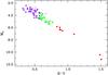 |
Fig. 1 HR diagram for the FGK stars of the DUNES sample observed by the DEBRIS team (DUNES_DB). The colour codes following the Hipparcos spectral types are F stars (violet), G stars (green), and K stars (red). Solid circles represent FGK stars closer than 20 pc; empty triangles are FGK stars further away. The two red dots at the bottom right of the diagram are two stars classified as K5 in the Hipparcos catalogue, but their colours correspond to M stars. See text for details. |
In Fig. 1 we show the HR diagram MV–(B − V) for the sample of FGK stars of the DUNES sample observed during the DEBRIS observing time. Solid circles represent FGK stars closer than 20 pc – i.e. the subsample analysed in this paper – whereas empty triangles have been used to plot FGK stars further away, not included in the study presented here. Two stars, namely HIP 84140 and HIP 91768 – the two red dots at the bottom right of the diagram – are both classified as K5 in the Hipparcos catalogue, but their (B − V) colours clearly correspond to that of an ~M3 star (the spectral type listed in SIMBAD for both objects), and so they have been moved out of the FGK star sample. We identify the subsample of 81 FGK stars as DUNES_DB in this paper, out of which 54 are closer than 20 pc. Table 1 summarizes the spectral type distribution of the DUNES_DU and DUNES_DB samples, taking into account these two misclassifications.
Table C.1 provides some basic information of the FGK stars within d ≤ 20 pc of the DUNES_DB sample (the corresponding information for the DUNES_DU sample can be found in Table 2 of E13). Hipparcos spectral types are given in the table. In order to check the consistency of these spectral types we have explored VizieR using the DUNES discovery tool6 (see Appendix A in E13). Results of this exploration are summarized in Col. 5 which gives the spectral type range of each star taken into account SIMBAD, Gray et al. (2003, 2006), Wright et al. (2003), and the compilation made by Skiff (2009). The typical spectral type range is 2−3 subtypes. The parallaxes are taken from van Leeuwen (2007, VizieR online catalogue I/311). Parallax errors are typically less than 1 mas. Only one star, HIP 46509, has an error larger than 2 mas, this object being a spectroscopic binary (see Table C.3). The multiplicity status of the DUNES_DB sample is addressed in Sect. 2.4.
2.2. Completeness
The main constraint affecting the completeness of the sample is the observational restriction that the photosphere had to be detected with a S/N ≥ 5 at 100 μm. It is important to know the impact of this restriction in order to assess the robustness of the results concerning the frequency of the incidence of debris discs in the solar neighbourhood.
In Fig. 2 the cumulative numbers of stars in the merged DUNES_DU and DUNES_DB d ≤ 15-pc and d ≤ 20-pc samples – normalized to the total number of objects in each one – have been plotted against stellar mass as red and blue histograms, respectively. The masses have been assigned to each star by linear interpolation of the values given for FGK MS stars by Pecaut & Mamajek (2013)7 using (B − V) as the independent variable. The expected mass spectrum for the solar neighbourhood according to a Salpeter law (Salpeter 1955) with exponent −2.35 has been normalized to the total cumulative number of each sample and plotted in green. It is clear that the sample with d ≤ 20 pc shows an underabundace of stars below ~1.2 M⊙, whereas the behaviour of the sample with d ≤ 15 pc approximates that of the Salpeter law, but still runs slightly below at low masses. Similar results are obtained using other approaches for the mass spectrum, e.g. that by Kroupa (2001). In grey, the cumulative distribution for the FGK stars with d ≤ 15 pc from the Hipparcos catalogue has also been included, showing a much closer agreement with the Salpeter law.
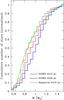 |
Fig. 2 Cumulative distributions (normalized) for the DUNES samples with d ≤ 15 pc (105 stars, red) and d ≤ 20 pc (177 stars, blue) and the FGK stars in the Hipparcos catalogue with d ≤ 15 pc (154 stars, grey), all plotted against stellar mass. A Salpeter law with exponent −2.35 has been normalized to the distributions. See text for details. |
Since the DUNES sample was drawn from the Hipparcos catalogue, it is important to assess the problem of its completeness. In Sect. 2.2 of Turon et al. (1992) it can be seen that the Hipparcos Input Catalogue was only complete down to V = 7.3 for stars cooler than G5. For d = 15 pc, this corresponds to a spectral type of ~K2. In addition, not all the stars in the Input Catalogue were observed (see Table 1 of Turon et al. 1992): for the magnitude bin V:7−8 the efficiency of the survey was 93%; therefore, even applying a safety margin of 0.3 mag, we would have completeness only up to spectral type K1. In summary, down to 15 pc, Hipparcos is complete for F and G stars, but not for K stars.
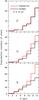 |
Fig. 3 Cumulative number of F, G, and K stars (luminosity classes V and IV−I) in the Hipparcos catalogue (red) and in the DUNES sample (black), both at d ≤ 15 pc. |
To quantify the departure of the full DUNES d ≤ 15-pc sample from the parent Hipparcos set, we compared the number of stars of each spectral type in our sample with the corresponding numbers in the Hipparcos catalogue. In Fig. 3, cumulative histograms of the numbers of F, G, and K stars (luminosity classes V and IV−V) in the Hipparcos catalogue (red), and in the DUNES sample (black), both at d ≤ 15, are plotted against distance. The total numbers of stars are 23 F, 42 G, 89 K in Hipparcos against 23 F, 33 G, 49 K in the DUNES sample, i.e. the observational constraint imposed in the final selection of the targets keeps all the F stars from Hipparcos, but discards 9 G and 40 K stars. Therefore, a correction on the fraction of excesses extracted from the DUNES sample would have to be applied – in particular for K stars – in order to give results referring to a wider sample. We come back to this point in Sect. 4.
2.3. Stellar parameters of the DUNES_DB sample
Table C.2 gives some parameters of the DUNES_DB objects with d< 20 pc, namely the effective temperature, gravity, and metallicity; the flag in Col. 5 indicates whether the determination of these parameters was spectroscopic or photometric. The stellar luminosity and the activity indicator  , are also given. References for Teff, log g, [Fe/H], and are at the bottom of the table. The luminosity was computed using Eq. (9) in Torres (2010), with the values of the V-magnitude and colour index (B − V) taken from the Hipparcos catalogue, and the bolometric corrections (BC) from Flower (1996); (B − V) was used as the independent variable to obtain BC.
The rotation periods, Prot, have been estimated using the strong correlation between and the Rossby number, defined as Ro = Prot/τc, where τc is the convective turnover time, which is a function of the spectral type (colour; Noyes et al. 1984; Montesinos et al. 2001; Mamajek & Hillenbrand 2008). For six objects, the estimation of Prot was not feasible because the calibrations do not hold for the values of either or B − V; in that case, lower limits of the rotation period, based on the values of vsini, are given. The stellar ages have been computed according to gyrochronology (tGyro) and using the chromospheric emission as a proxy for the age (tHK). In Appendix A we give details of the estimation of the rotation periods and ages.
2.4. Multiplicity
Table C.3 lists the multiplicity properties of the objects that are known to be binaries. The importance of this information cannot be underestimated, especially when the spectral types of the components are close – and hence ΔV is small – and the binary is spectroscopic or its components have not been resolved individually during a particular spectroscopic or photometric observation from which a given parameter is derived. In many cases parameters are assigned as representative of the whole system, without reference in the literature to which component they refer to. This also has an impact on the calculation of the corresponding model photospheres that are used (after normalization to the optical and near-IR photometry) as baselines to detect potential excesses at the Herschel wavelengths. Concerning the data given in Table C.3, this has to be taken into account for HIP 7751 (ΔV = 0.16), HIP 44248 (1.83), HIP 61941 (0.04), HIP 64241 (0.68), HIP 72659 (2.19), HIP 73695 (0.87), and HIP 75312 (0.37), and for those stars classified as “spectroscopic binaries” for which no information on their components is available. The proper motions of the components have been extracted from the “Hipparcos and Tycho catalogues (Double and Multiples: Component solutions)” (VizieR online catalogue I/239/h_dm_com).
The bottom part of Table C.3 gives information about the stars of the DUNES_DB sample with d ≤ 20 pc that to date have confirmed exoplanets. The mass and the length of the semimajor axis of the orbit for each planet are given.
2.5. Photometry
Tables C.4–C.7 give the optical, near-IR, AKARI, WISE, IRAS, and Spitzer MIPS magnitudes and fluxes of the DUNES_DB stars with d ≤ 20 pc, and the corresponding references. This photometry has been used to build and trace the spectral energy distributions (SEDs) of the stars, which are – along with PHOENIX/Gaia models (Brott & Hauschildt 2005) – the tools used to predict the fluxes at the far-IR wavelengths in order to determine whether or not the observed fluxes at those wavelengths are indicative of a significant excess. Appendix C in E13 gives details on the photospheric models and the normalization procedure to the observed photometry. In addition to the photometry, Spitzer/IRS spectra of the targets, built by members of the DUNES consortium from original data from the Spitzer archive, are included in the SEDs, although they have not been used in the process of normalization of the photospheric models.
3. Herschel observations of the DUNES_DB sources and data reduction
3.1. PACS observations
As described by Matthews et al. (2010), DEBRIS is a flux-limited survey where each target was observed to a uniform depth (1.2 mJy beam-1 at 100 μm). The observations of the DUNES_DB sources were performed by the DEBRIS team with the ESA Herschel Space Observatory using the instrument PACS. Further details can be found in the paper by Matthews et al. (2010). The main parameters of the observational set-up used by DEBRIS are compatible with those used by DUNES and are described in E13.
3.2. Data reduction
Data for each source comprise a pair of mini scan-map observations taken with the PACS 100/160 waveband combination. DEBRIS and DUNES observations both followed the same pattern for mini scan-map observations (see PACS Observer’s Manual, Chap. 5); minor differences in the scan leg lengths (8′ for DEBRIS, 10′ for DUNES) lead to slightly different coverage across the resulting map areas for the two surveys, in addition to the different map depths. These differences are immaterial to the analysis presented here. The Herschel/PACS observations were reduced in the Herschel interactive processing environment (HIPE, Ott 2010). For the analysis presented here we used HIPE version 10 and PACS calibration version 45. Reduction was carried out following the same scheme as presented in E13. Table C.8 shows a log of the observations with details of the OBSIDs and the on-source integration times.
The individual PACS scans of each target were high-pass filtered to remove large-scale background structure, using high-pass filter radii of 20 frames at 100 μm and 25 frames at 160 μm, suppressing structures larger than 82′′ and 102′′, respectively, in the final images. For the filtering process, a region of 30′′ radius around the source position in the map along with regions where the pixel brightness exceeded a threshold defined as twice the standard deviation of the non-zero flux elements in the map (determined from the level 2 pipeline reduced product) were masked from inclusion in the high-pass filter calculation. Regions external to the central 30′′ that exceeded the threshold were tagged as sources to be avoided in the background estimation phase of the flux extraction process. Deglitching was carried out using the spatial deglitching task in median mode and a threshold of 10σ. For the image reconstruction, a drop size (pixfrac parameter) of 1.0 was used. Once reduced, the two individual PACS scans in each waveband were mosaicked to reduce sky noise and suppress 1/f striping effects from the scanning. Final image scales were 1′′ per pixel at 100 μm and 2′′ per pixel at 160 μm, compared to native instrument pixel sizes of 3.2′′ for 100 μm, and 6.4′′ for 160 μm.
4. Results
The extraction of PACS photometry of the sources analysed in this paper follows identical procedures to those in E13. Section 6.1.1 of that paper contains a very detailed description of the procedures used to carry out the flux extraction. In summary, flux densities were measured using aperture photometry. If the image was consistent with a point source, then an aperture appropriate to maximise the signal-to-noise was adopted (i.e. 5′′ at 100 μm and 8′′ at 160 μm; see E13). Regarding extended sources, we refer the reader to Sect. 7.2.3 of E13 where the criteria are described for assessing whether the 3σ flux contours in the 100 and 160 μm images denote extended emission.
The background and rms scatter were estimated from the mean and standard deviation of ten square sky apertures placed at random around the image. The sky apertures were sized to have roughly the same area as the source aperture. The locations of the sky apertures were chosen such that they did not overlap with the source aperture or with any background sources (to avoid contamination), and lay within 60′′ of the source position (to avoid higher noise regions at the edges of the image).
Measured flux densities in each PACS waveband were corrected for the finite aperture size using the tabulated encircled energy fractions given in Balog et al. (2014), but have not been colour corrected8. A point-source calibration uncertainty of 5% was assumed for all three PACS bands. We note that aperture corrections valid for point sources have also been applied to the case of extended sources. This is obviously an approach, but it should be valid as long as the aperture size is larger than the extended source. This criterion has widely been used without any apparent inconsistency in other works, e.g. Wyatt et al. (2012) for 61 Vir, Duchêne et al. (2014) for η Crv, and Roberge et al. (2013) for 49 Cet.
Table C.9 lists the PACS 100 and 160 μm photometry and 1σ uncertainties for the sources of the DUNES_DB sample with d ≤ 20 pc, identified as the far-IR counterparts of the optical stars. Uncertainties include both the statistical and systematic errors added in quadrature; the uncertainty in the calibration is 5% in both bands (Balog et al. 2014). Quantities without errors in the PACS160 column correspond to 3σ upper limits. In the columns adjacent to the PACS photometry, the photospheric predictions, Sν(λ), with the corresponding uncertainties are given. The fluxes Sν(λ) are extracted from a Rayleigh-Jeans extrapolation of the fluxes at 40 μm from the PHOENIX/Gaia normalized models. The uncertainties in the individual photospheric fluxes were estimated by computing the total σ of the normalization in logarithmic units; in that calculation, the observed flux at each wavelength involved in the normalization process was compared with its corresponding predicted flux. The normalized model log Sν(λ) was permitted to move up and down a quantity ± σ. That value of σ was then translated into individual – linear – uncertainties of the fluxes, σ(Sν(λ)), at the relevant Herschel wavelengths. The typical uncertainty in the photospheric predictions derived from a change of ± 50 K in Teff for a model with 6000 K is ~0.9% of the predicted flux density. It does not have noticeable effects in any of the calculations.
We consider that an object has an infrared excess at any of the PACS wavelengths when the significance, calculated as  (1)
(1)
is larger than 3.0, although in some cases the complexity of the fields makes it difficult to ascertain whether an apparent clear excess based solely on the value of χλ is real or not.
The values of χ100 and χ160 are listed in Table C.9 along with the status “Excess/No excess” or “Dubious” in the last column, derived from these numbers and from a careful inspection of the fields. In addition, PACS 70 μm and SPIRE photometry from the literature were included for HIP 61174, HIP 64924, and HIP 88745, and PACS 70 μm photometry for HIP 15510. The fluxes and the corresponding references are given at the bottom of Table C.9.
4.1. Stars with excesses
After a careful analysis of the corresponding images and surrounding fields, 11 stars of the DUNES_DB sample with d ≤ 20 pc show real excesses among those in Table C.9 having χ100 and/or χ160> 3.0. They are listed in the upper half of Table 2.
Eight sources show excess at both 100 and 160 μm; they are HIP 15510, HIP 16852, HIP 57757, HIP 61174, HIP 64924, HIP 71284, HIP 88745, and HIP 116771.
Black-body dust temperatures and fractional dust luminosities for the DUNES_DB stars with excesses.
Two sources, HIP 5862 and HIP 23693, show excess only at 100 μm and fluxes at 160 μm slightly above the photospheric flux, but not large enough to give χ160> 3.0. Consequently, they present a decrease in their SED for λ ≥ 100μm, similar to those in three stars in DUNES_DU (HIP 103389, HIP 107350, and HIP 114948). An extensive modelling of these three objects was done by Ertel et al. (2012) and their conclusions can be applied to HIP 5862 and HIP 23693.
HIP 113283 shows excess only at 160 μm; therefore, it is a cold-disc candidate like those discovered and modelled by Eiroa et al. (2011), E13, Krivov et al. (2013), and Marshall et al. (2013).
Among the 11 sources with confirmed excesses, five have been spatially resolved. They are marked with an asterisk in Tables 2 and C.9. Four of them were already known, namely HIP 15510 (Wyatt et al. 2012, Kennedy et al. 2015), HIP 61174 (Matthews et al. 2010; Duchêne et al. 2014), HIP 64924 (Wyatt et al. 2012), and HIP 88745 (Kennedy et al. 2012).
The fifth extended source found in this work is HIP 16852. A two-dimensional Gaussian fit gives full widths at half maximum (FWHM) along the principal axes of 7.7′′ × 8.5′′ at 100 μm and 12.2′′ × 10.5′′ at 160 μm, where those of the PSF along the same directions at each wavelength are 6.9′′ × 6.8′′ and 11.8′′ × 10.9′′, respectively. This implies that the source is marginally resolved at 100 μm. Thus, HIP 16852 is similar in terms of angular size to HIP 15510, which was also marginally resolved at 100 μm by Kennedy et al. (2015)9.
Among the excess sources, planets have been detected around HIP 15510 (Pepe et al. 2011), and HIP 64924 (Vogt et al. 2010), see details in Table C.3.
In addition to the excess sources, nine more objects have χ100 and/or χ160> 3.0, but are labelled in Table C.9 as “Dubious” because of the complexity of the fields that makes an unambiguous measurement of the fluxes difficult. They are listed in the lower half of Table 2: HIP 1599, HIP 36366, HIP 44248, HIP 37279, HIP 59199, HIP 61941 (all of them F-type), HIP 72659, HIP 73695 (binaries with a primary of G-type), and HIP 77257 (G).
In Table 2, we give the results for TBB, estimated from black-body fittings, and the fractional luminosity Ldust/L∗ computed by integrating directly on the one hand the black-body curve that best fits the excess, and on the other, the normalized photospheric model. Values are given both for the stars with confirmed and apparent excesses. Typical uncertainties in the black-body temperatures are ± 10 K. For all the stars, apart from HIP 61174, the data involved in the black-body fittings are only the PACS – and SPIRE, if available – flux densities. For HIP 61174, the fit to the warm black body includes all the ancillary photometry between 10 and 30 μm (WISE W3 and W4, Akari 18, MIPS 24, IRAS 12 and 25) collected by us and listed in Tables C.6 and C.7.
The values of the fractional luminosity that appear in the table for HIP 5862 and HIP 23693 correspond to modified black-body fits to all the points showing excess; however, those fits have been used just to integrate the excess fluxes, since the values of β – the parameter modifying the pure black body in (λ0/λ)β – are unreasonably high in both cases, of the order of ~6.0, making a physical interpretation very difficult; most probably a two-ring disc would be more adequate to model those two cases. The black-body radii computed according to the expression
 (2)
(2)
(see e.g. Backman & Paresce 1993) are also included in the table.
Figures B.1 and B.2 show the SEDs of the sources with confirmed and dubious excesses, respectively. In blue we have plotted all the photometry available below 70 μm, in red the PACS fluxes – and the SPIRE values for some objects, in black the model photosphere normalized, and in green the black-body fits to the excess.
Information for some of these sources has been already reported in other works. Gáspár et al. (2013) compiled a catalogue of Spitzer/MIPS 24 and 70 μm, and Herschel/PACS 100 μm observations that includes the stars analysed in this paper. They confirm excesses for 7 out of the 11 stars listed at the top of Table 2, the exceptions being HIP 57757 (χ100 = 1.01) and HIP 71284 (χ100 = 3.35, but no MIPS data available); HIP 113283 is obviously labelled as “no-excess” by these authors because they did not analyse the observation at 160 μm, the wavelength where we detect an excess. For HIP 116771 they do not provide the PACS 100 μm flux and the star is catalogued as a non-excess source according to the MIPS 70 μm (χ70 = 1.77).
Chen et al. (2014) analysed and modelled the SEDs of 499 targets that show Spitzer/IRS excesses, including a subset of 420 targets with MIPS 70 μm observations. They found that the SEDs for the majority of objects (~66%) were better described using a two-temperature model with warm (Tdust ~ 100−500 K) and cold (Tdust ~ 50−150 K) dust populations analogous to zodiacal and Kuiper Belt dust. Four of their excess sources – for which we also find an excess in the far-IR – appear in Chen et al. (2014, VizieR online catalogue J/ApJS/211/25): HIP 5862, HIP 23693, and HIP 64924 are modelled with two-temperature fits, the cold components having Tdust = 94 ± 8, 51 ± 7, and 54 ± 10 K, respectively, whereas HIP 16852 is reproduced by a one-temperature fit with Tdust = 100 ± 6 K. The single black-body fits for those stars (see Table 2) are 96, 82, 50, and 87 K, respectively, which do not deviate much from the determinations by Chen et al.
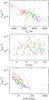 |
Fig. 4 Upper limits of the fractional luminosity of the dust for the non-excess sources of the DUNES_DB (crosses) and the DUNES_DU (dots) samples within 20 pc, plotted against the effective temperature, distance, and stellar flux at 100 μm. Violet, green, and red represent F, G, and K stars. See text for details. |
Moro-Martín et al. (2015) also reported the detection or non-detection of dust around stars of the DUNES and DEBRIS samples based solely on their measurements of the Herschel/PACS 100 μm fluxes. Eight out of the 11 stars we claim as having excess match their positive detections, the exception being HIP 57757, for which they find a χ100 = 2.43, and HIP 113283, for which we only detect excess at 160 μm, as pointed out above; HIP 88745 does not appear in their sample.
Since the observed excess emission of some disc candidates is relatively weak, the possibility of contamination by background galaxies cannot be excluded (E13, Krivov et al. 2013). Sibthorpe et al. (2013) carried out a cosmic variance independent measurement of the extragalactic number counts using PACS 100 μm data from the DEBRIS survey. To estimate the probability of galaxy source confusion in the study of debris discs, Table 2 of that paper gives the probabilities of one background source existing within a beam half-width half-maximum radius (3.4′′ for PACS 100, 5.8′′ for PACS 160) of the measured source location for a representative range of excess flux densities.
We have computed the excess flux densities at 100 and 160 μm for the 11 discs in Table 2. The smallest values at each wavelength occur for HIP 15510 (8.0 mJy) and HIP 113283 (7.8 mJy). These values imply the probability of coincidental alignment with a background object of 0.2% and 1%, respectively. Since the excess flux densities are larger for the remaining targets, the probabilities for them are obviously lower.
In the case of a survey, it is more relevant to ask what the probability is that one or more members of the sample coincide with a galaxy. We have computed the median 1σ uncertainties – only considering the rms of the measurement, not the calibration error – of the PACS 100 and 160 μm fluxes for the set of 54 stars of the DUNES_DB sample within 20 pc, the results being 1.63 and 3.18 mJy, respectively. Assuming fluxes for potential background sources of three times those σ values at the corresponding wavelengths, we obtain at 100 μm a chance of coincidental alignment for a single source of 1.1%. This implies the following binomial probabilities P(i) of having i fakes in the sample of 54 stars: P(0) = 55%, P(1) = 33%, P(2) = 10%, P(3) =2%, and P(4) = 0.3%. For 160 μm, the chance of coincidental alignment of a single source is 2.9%, which implies P(0) = 21%, P(1) = 33%, P(2) = 26%, P(3) = 13%, and P(4) = 5%. Equation (2) of the paper by Sibthorpe et al. (2013) and the matrices provided in that work were used to compute these estimates.
As we pointed out, 5 of the 11 excess sources found in this work are spatially resolved; therefore, we can consider them to be real debris disc detections. According to the results above, the chances that the remaining six sources were all contaminated by background galaxies are ~0.003% and ~0.4% at 100 and 160 μm, respectively.
4.2. Stars without excesses
Figure B.3 shows the SEDs of the DUNES_DB stars within 20 pc without excesses. In Fig. 4 the 3σ upper limits of the fractional luminosity of the dust for these sources are plotted as crosses against the effective temperature, distance, and stellar flux at 100 μm. For the sake of completeness, the non-excess DUNES_DU sources within 20 pc have been also added (dots; see Fig. 8 and Table 12 of E13). Violet, green, and red represent F, G and K stars. The dubious sources are not included. The upper limits have been computed using the PACS 100 μm flux densities in expression (4) in Beichman et al. (2006), with a representative Tdust = 50 K.
The plots in Fig. 4 confirm and extend what was already seen in E13. The upper panel shows that the upper limits tend to decrease with Teff, the middle panel shows that for a given distance the hotter the star the lower the upper limit, and the lower panel shows that for a given predicted photospheric flux, which depends both on the spectral type and the distance, the upper limits increase with decreasing effective temperature. The general trend of the Ldust/L∗ upper limits decreasing with the stellar temperature is expected just from pure black-body scaling considerations and the construction of the DUNES survey. Finer details, however, depend on the particular depth achieved for different spectral types and each individual observation.
The lowest values of the upper limits for the fractional luminosity reached are around ~4.0 × 10⁻⁷; the median for each spectral type are 7.8 × 10⁻⁷, 1.4 × 10⁻⁶, and 2.2 × 10⁻⁶ for F, G, and K stars, respectively; the median for the whole sample is 1.4 × 10⁻⁶.
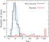 |
Fig. 5 Plotted in black, the histogram of the 100 μm significance χ100 for the non-excess sources of the merged DUNES_DU and DUNES_DB samples with d ≤ 20 pc (dubious sources of both samples are not included). A Gaussian with σ = 1.40, the standard deviation of the χ100 values for these sources, is plotted in blue. In cyan, we show a Gaussian with σ = 1.02, corresponding to the subsample of non-excess sources with −2.0 <χ100< 2.0. In red, the distribution of χ100 for the excess sources is also displayed. This figure is an extension of Fig. 6 in E13. See text for details. |
In Fig. 5 histograms of the significance χ100 for the non-excess (black) and excess (red) sources of the merged DUNES_DU and DUNES_DB samples with d ≤ 20 pc are plotted. For the non-excess sources, the mean, median, and standard deviation of the χ100-values are −0.23, −0.33, and 1.40, respectively. A Gaussian curve with σ = 1.40 is also plotted. These results are an extension of those already presented in Sect. 7.1 and Fig. 6 of E13, and are quantitatively very similar. The shift to the peak of the distribution to a negative value of χ100 likely reflects the fact that the extrapolation of the model photospheres to the PACS bands using a Rayleigh-Jeans approximation does not take into account the decrease in brightness temperature at ~100μm that occurs in late-type stars, and therefore overestimates the photospheric emission around that wavelength. This was directly observed using DUNES data for α Cen A (Liseau et al. 2013) and α Cen B (Wiegert et al. 2014). We note that the stars in the red histogram with χ100< 3.0 are those considered to harbour a cold disc, the excess being present only at 160 μm.
The fact that the standard deviation of the distribution departs from 1.0 – the expected value assuming a normal distribution – poses a problem already encountered in e.g. E13 and Marshall et al. (2014). One potential origin of this could be the underestimation of the uncertainties either in the PACS 100 μm flux, in the photospheric predictions, or both, which would have the effect of increasing the absolute values of χ100 since the term containing the uncertainties is in the denominator of the definition of χλ (Eq. (1)). The distribution of χ100 would become broader, and σ would increase. We have done the experiment of computing the mean, median, and σ for the non-excess sources considering only those stars with values of −2.0 <χ100< 2.0, the goal being to test the central part of the distribution. The results for the three quantities for this subset of stars (108 objects) are −0.28 (mean), −0.34 (median), and σ = 1.02 (Gaussian curve plotted in cyan in Fig. 5). This shows that the problem is more complex than dividing the stars into two bins of “excess” and “non-excess”. There must be a spectrum of values with an increasing contribution from dust to the total measurement in the non-excess sample until it hits a threshold and becomes an excess value, which has been set in practice to χλ = 3.0. This can have the effect of a departure of the full distribution from normal; instead, narrowing the interval of χ100, ensuring that we deal with a more conservative definition of non-excess sources, seems to have the effect of approaching a normal distribution.
Summary of stars per spectral type in the DUNES_DU and DUNES_DB samples and frequency of excesses.
5. Analysis of the full DUNES sample
In E13 some conclusions were drawn based solely on the DUNES_DU subsample. In this section we comment on the relevant results that are derived from the analysis of the merged DUNES_DU + DUNES_DB sample, both with d ≤ 15 pc and d ≤ 20 pc.
5.1. Excess incidence rates
Table 3 shows a summary of the excess incident rates in the DUNES_DU, DUNES_DB, and the full sample. In particular, the d ≤ 15-pc subsample contains 23 F, 33 G, and 49 K stars. The incidence rates of excesses are 0.26 (6 objects with excesses out of 23 F stars), 0.21 (7 out of 33 G stars), and 0. 20 (10 out of 49 K stars), the fraction for the total sample with d ≤ 15 pc being 0.22 (23 out of 105 stars). Those percentages do not change significantly if we consider all targets within d ≤ 20 pc. We also give the 95% confidence intervals for a binomial proportion for the corresponding counts according to the prescription by Agresti & Coull (1998).
As specified in Sect. 4.2, the median of the upper limits of the fractional luminosities per spectral type are 7.8 × 10⁻⁷, 1.4 × 10⁻⁶, and 2.2 × 10⁻⁶ for F, G, and K stars, respectively. As mentioned in E13, these numbers improve the sensitivity reached by Spitzer by one order of magnitude. Our results are to be compared with those found by Trilling et al. (2008, see Table 4 of their paper), where the incidence rates of stars with excess at 70 μm as measured by Spitzer/MIPS are 0.18, 0.15, and 0.14 for F, G, and K stars, respectively. The variation of the incidence rates with spectral type is likely directly related to the dependence of the fractional luminosity with Teff (see Fig. 4).
As we showed in Sect. 2.2, the merged sample with d ≤ 15 pc analysed in this paper is complete for F stars and almost complete for G stars, whereas a number of K stars have been lost from the parent set of the Hipparcos catalogue from which the final DUNES sample was drawn, the reason being the observational constraint imposed (background contamination; see Sect. 2.1). In the bottom row of Table 3 we give the expected total number of stars of each spectral type in the Hipparcos catalogue with d ≤ 15 pc that would show excess, under the assumption that the individual excess frequencies are those obtained from the full DUNES sample; the numbers that are extrapolations for the G and K stars are written in italics. The total incidence rate of excesses for the Hipparcos subset, namely  , does not change with respect to the DUNES result,
  , the confidence interval being obviously slightly narrower. Since both τ Cet and ϵ Eri are within 15 pc and have debris discs (Lawler et al. 2014; Greaves et al. 2014), if these sources were included in the statistics, the total incidence rate of excesses within d ≤ 15 pc would be
  (25 out of 107 objects).
The results on the incidence rates of excesses from PACS data allows us to push the distribution found from MIPS data, whose minimum detection limit was Ldust/L∗ ≃ 4 × 10⁻⁶ (Bryden et al. 2006), down to minimum detections around 4 × 10⁻⁷. Figure 6 shows a cumulative distribution of the frequency of excess detections from PACS data as a function of the fractional dust luminosity. The steepness of the distribution decreases at luminosities lower than ~4 × 10⁻⁶. The extrapolation of a straight line fitted to the bins at the left of that value predicts an incidence of excesses ~0.25 at Ldust/L∗ = 10-7, the current estimate of the Kuiper-belt dust fractional luminosity (Vitense et al. 2012). The cumulative distribution of the frequency of excesses derived from the results shown in Tables 2 and 3 of Bryden et al. (2006, 11 excesses out of 73 stars) is also included in Fig. 6; these were obtained from Spitzer/MIPS observations at 70 μm, with a detection limit of Ldust/L∗ ≃ 4 × 10⁻⁶. The shape of both distributions is roughly the same in the range ~4 × 10⁻⁶−3 × 10⁻⁵. A straight line fitted to the bins of our cumulative histogram in that region would predict a larger incidence of excesses ~0.35, at fractional luminosities of 10-7. A very similar prediction (~0.32) is obtained from the cumulative histogram by Bryden et al. (2006).
The fact that the Spitzer/MIPS and Herschel/PACS distributions are close to each other in the overlapping range of luminosities is more than a simple consistency check. The similarity might indicate that the dust temperature does not correlate with the dust luminosity in that range. The dust fractional luminosities in Bryden et al. (2006) were based either on a single 70 μm measurement or on a combination of 24 μm and 70 μm fluxes. The dust luminosities in this work were derived from fluxes at longer wavelengths, basically from 70 μm, 100 μm, and 160 μm PACS fluxes. For simplicity, we assume that the Spitzer luminosities were based solely on a 70 μm flux and the Herschel values solely on a 100 μm flux. Under this assumption, the fractional luminosity is directly proportional to the flux at 70 μm or 100 μm (see Eq. (3) in Bryden et al. 2006). Next, it is obvious that the F70/F100 ratio decreases with decreasing dust temperature. Should the discs with lower fractional luminosities be systematically colder, the F70/F100 flux ratio would decrease with the dust luminosity. This would make the histogram based on F70 flux flatter and conversely, the histogram based on the F100 flux steeper. In the opposite case, i.e. if the discs of low fractional luminosity were systematically warmer, the opposite would be true. In either case, the slopes of the two histograms would differ, but this is not what we see in Fig. 6; instead, they are nearly the same in the ~4 × 10⁻⁶−3 × 10⁻⁵ luminosity range. Therefore, the dust temperature should be nearly the same for all discs with the dust luminosities in that range.
What implications might this have? The dust temperature is directly related to the disc radius. Assuming that the average stellar luminosity of all stars with discs in that fractional luminosity range is nearly the same, the fact that the dust temperature does not depend on the dust luminosity would automatically mean that the disc radius does not depend on the dust luminosity either. This would imply that it is not the location of the dust-producing planetesimals that primarily determines the disc dustiness. Instead, the disc dustiness must be set by other players in the system, e.g. by the dynamical evolution of presumed planets in the disc cavity.
The bottom line of this analysis is that the flattening of the distribution at low values of Ldust/L∗ provided by the results of the Herschel observations decreases drastically the predictions of the excess incidence rate at luminosities ~10-7 compared to those obtained from MIPS results.
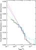 |
Fig. 6 Cumulative distributions of the frequency of excesses obtained in this work (black) and those obtained from Spitzer/MIPS results Bryden et al. (2006; cyan), both plotted against fractional dust luminosity. The green straight line is a fit to the values of the frequencies at the less steep part of our cumulative distribution. The extrapolation down to 10-7, the current estimate of the Kuiper-belt fractional luminosity, gives a prediction for the incidence rate of excesses of ~0.25. The extrapolation from a straight line, plotted in red, fitted to the steeper part of the distribution, that mimics the MIPS results, gives a higher prediction ~0.35. The prediction from the Bryden et al. (2006) distribution, from the blue straight-line fit, is ~0.32. See text for details. |
5.2. Debris discs/binarity
Figure 7 shows the projected binary separation versus disc radius for excess sources in those stars catalogued as binaries in Table C.3 of this work (red symbols) as well as those in E13 (Table 16 of that paper, blue symbols). Squares and diamonds represent confirmed and dubious excess sources, respectively; triangles mark the spectroscopic binary HIP 77257, which has an unknown – but presumably small – separation. Filled and open symbols connected with an arrow represent the black-body disc radius, RBB computed using Eq. (2) and a more realistic disc radius estimate, Rdust, according to Pawellek & Krivov (2015), respectively, for the same system10.
The discs above the diagonal straight line are circumprimary, those below the line circumbinary. The grey area roughly marks the discs that are not expected to exist as they would be disrupted by the gravity of the companion (assuming the true distance to be close to the projected one). There is no apparent reason why all the red symbols, which correspond to stars in the DUNES_DB sample, lie in the “circumbinary” region. The ranges of the disc radii in DUNES_DU and DUNES_DB are similar, it is only the distributions of the binary separations that are different (more wide binaries in the DUNES_DU sample); whether a wide or a close binary is found among the excess sources in one of the samples seems to be purely accidental.
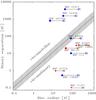 |
Fig. 7 Projected binary separation plotted against disc radius for excess sources in those stars catalogued as binaries. Red and blue symbols represent objects studied in this work and in E13, respectively. Squares and diamonds are confirmed or dubious excesses. Filled and open symbols represent the value of RBB and Rdust (see text for details). The inverted triangles at the bottom represent the binary HIP 77257 for which the separation is not known. |
5.3. Debris discs/metallicity
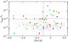 |
Fig. 8 Fractional dust luminosities Ldust/L∗ for the DUNES_DU and DUNES_DB stars with excesses (squares) and d ≤ 20 pc (Table 14 in E13 and Table 2 in this work), and upper limits for the non-excess sources (crosses), all of them plotted against metallicity, [Fe/H]. F, G, and K stars are plotted in violet, green, and red. The short-dashed vertical line marks the mean metal abundance of the whole sample, [Fe/H] = −0.11, whereas the long-dashed line marks the median, [Fe/H] = −0.095. The horizontal lines mark the means (solid) of the fractional luminosities for the debris discs of stars showing excess, with [Fe / H] ≤ −0.11 and >−0.11, and plus and minus their standard errors (dotted), defined as σ/ |

In Fig. 8, the fractional luminosities Ldust/L∗ (for the excess sources) and the upper limits (non-excess sources) for the full DUNES sample with d ≤ 20 pc are plotted against stellar metallicity. It is interesting to note that whereas above the mean metal abundance of the whole sample, [Fe/H]mean = −0.11, we find a wide range of values of the fractional luminosity covering more than two orders of magnitude, the discs around stars with [Fe/H] below −0.11 seem to show a much narrower interval of Ldust/L∗, around ~10-5. Two statistical tests performed on the data, namely the Kolmogorov-Smirnov and the Anderson-Darling, state that the result is not statistically significant; therefore, a larger sample is needed to confirm or discard this trend.
Greaves et al. (2006) and Beichman et al. (2006) found that the incidence of debris discs was uncorrelated with metallicity; these results have been confirmed by Maldonado et al. (2012, 2015) who find no significant differences in metallicity, individual abundances, or abundance-condensation temperature trends between stars with debris discs and stars with neither debris nor planets. However, Maldonado et al. (2012) have pointed out that there could be a deficit of stars with discs at very low metallicities (−0.50 < [Fe / H] < −0.20) with respect to stars without detected discs. A recent work by Gáspár et al. (2016), where the correlation between metallicity and debris disc mass is studied, has confirmed the finding by Maldonado et al. (2012) of a deficit of debris-disc-bearing stars over the range −0.5 ≤ [Fe / H] ≤ −0.2. Out of the full sample analysed in this paper, 166 stars have determinations of their metallicities, all of which are plotted in Fig. 8; the number of stars with excesses at both sides of the median metallicity, [Fe/H]median = −0.095, is 16 ([Fe / H] < −0.095) and 20 ([Fe / H] > −0.095), i.e. a slightly lower proportion on the low-metallicity side. Considering an average uncertainty of ± 0.05 dex in the metallicities that could move objects from one to the other side of the boundary marked by the median, we can count the number of debris discs around stars with metallicities lower than [Fe/H]median − 0.05 and higher than [Fe/H]median + 0.05, the results being 11/83 and 15/83 objects, respectively. The fractions are 0.13 and 0.18
 , respectively, with the uncertainties corresponding to a 95% confidence level. Although this result is still not statistically significant, it points in the same direction as the values hinted by Maldonado et al. (2012) and confirmed by Gáspár et al. (2016).
Statistics of the dust fractional luminosities.
5.4. Evolutionary considerations
Figure 9 shows a plot of against (B − V) for the DUNES stars within 20 pc, plotted as cyan squares. The stars with excesses are plotted as diamonds with sizes proportional to log Ldust/L∗. The regions separating “very inactive”, “inactive”, “active”, and “very active” stars proposed by Gray et al. (2006, see their Fig. 4) are also indicated. This diagram is a qualitative evolutionary picture of FGK main sequence stars in the sense that as the stars evolve, their rotation rates decrease as a consequence of angular momentum loss and therefore their levels of chromospheric activity also decrease (see e.g. Skumanich 1972; Noyes et al. 1984; Rutten 1987).
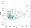 |
Fig. 9 Diagram of |
Out of the 177 stars of the DUNES sample with d ≤ 20 pc, 175 have data; 119 objects (25 showing excesses, 21.0%) are in the region of “inactive” or “very inactive” stars ( , “old” objects), whereas 56 (11 with excesses, 19.6%) are in the region of the “active” or “very active” stars (
 , “young” objects). This means that the incidence of debris discs is similar among inactive and active stars.
The uneven distribution of stars below and above the activity gap is more apparent if we use large samples of field FGK stars to check the relative abundance of active and inactive objects in the solar neighbourhood. Two catalogues have been used to ascertain this point: the Henry et al. (1996) catalogue contains 814 southern stars within 50 pc, most of them G dwarfs. From the Gray et al. (2006) catalogue, which contains stars within 40 pc, we have retained those FGK stars with luminosity classes V or V−IV (1270 objects). The stars of both surveys have been plotted as grey crosses in Fig. 9. The bimodal distribution in stellar activity first noted by Vaughan & Preston (1980) in a sample of northern objects is seen in both catalogues, the percentage of inactive stars below the gap frontier at  is 73% (Henry et al. 1996) and 64% (Gray et al. 2006) for B − V< 0.85. For the sample in this paper, the percentage of stars below
  is 68%.
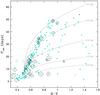 |
Fig. 10 Diagram of Prot – (B − V) showing the stars of the full DUNES sample with d ≤ 20 pc (cyan squares). As in Fig. 9 the stars identified as having far-infrared excesses are plotted as diamonds with a size proportional to the value of the fractional dust luminosity. Superimposed are five gyrochrones computed following Mamajek & Hillenbrand (2008; see Appendix A in this work). |
Figure 10 shows the rotation periods (see Table C.2) plotted against the (B − V) colours for the DUNES stars within 20 pc. Five gyrochrones corresponding to 0.6, 1.0, 2.5, 5.0, and 7.5 Gyr, computed according to Mamajek & Hillenbrand (2008) are also included in the graph. The stars with excesses are plotted as black diamonds with sizes proportional to log (Ldust/L∗). In spite of the problems involved in the estimation of ages, the reliability of the computation of rotation periods from the chromospheric activity indicator (see Appendix A) makes this diagram a reliable evolutionary scenario of how the sample and the excess sources are distributed.
In Fig. 9 it is apparent that the sizes of the diamonds above the line are, on average, larger than those below; the line separates active (younger) from inactive (older) stars. In turn, in Fig. 10 it can be also seen that the average sizes of the symbols decrease as the rotation periods increase, suggesting a decreasing fractional luminosity with increasing stellar age.
To quantify this, we have taken two bins in chromospheric activity, namely stars above and below , and three bins in rotation period, Prot< 10 d, 10 d<Prot< 30 d, and Prot> 30 d, and have determined means and medians of the dust fractional luminosities of the stars in each bin. The results of this exercise can be seen in Table 4 where the calculations have been carried out for the whole sample (d ≤ 20 pc). Stars with upper limits in Ldust/L∗ (three objects in the DUNES_DU sample and one in DUNES_DB) and with lower limits in Prot (four objects) have not been included; in the last column N specifies the number of stars used in each case. The effects of decreasing Ldust/L∗ with decreasing activity and increasing rotation period are apparent. These results show that as the stars get older there seems to be a slow erosion of the mass reservoir and dust content in the disc, with the effect of a decrease in Ldust/L∗. An extensive and more detailed study on the evolution of debris discs was carried out by Sierchio et al. (2014).
6. Summary
The main goal of this paper – and of the DUNES project – is to study the incidence of debris discs around FGK stars in the solar neighbourhood. Data obtained with the ESA Herschel space observatory have been used to characterize the far-IR SED of a sample of objects observed during two Open Time Key Programmes, DUNES and DEBRIS. A sample of 177 stars within 20 pc has been analysed.
Figure 11 shows the fractional dust luminosity, Ldust/L∗, plotted against the dust temperature, Tdust, for the 36 stars for which a far-IR excess has been detected (see Table 14 in E13 and Table 2 in this work). The detection limits for a G5 V star at 20 pc, following Bryden et al. (2006), are also included in the graph; the assumed 1σ fractional flux accuracies are 20% for Spitzer/MIPS at 70 μm and 10% for Herschel/PACS at 100 μm (i.e. S/N = 10). Fourteen stars are located below the MIPS 70 μm curve, showing how Herschel/PACS has pushed the limits down to fractional luminosities that are a few times that of the Kuiper-belt.
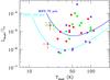 |
Fig. 11 Diagram of Ldust/L∗ – Tdust showing the position of the 36 stars, out of the 177 in the DUNES sample within 20 pc, for which an excess has been detected at far-IR wavelengths. F, G, and K stars are plotted in violet, green, and red. The detection limits for a G5 V star at 20 pc for PACS 100 μm and MIPS 70 μm are also included. |
A summary of the main results follows:
-
1.
Herschel/PACS photometry – complemented in some cases with SPIRE data – are provided for the so-called DUNES_DB sample, a set of 54 stars (32 F, 16 G, and 6 K) observed by DEBRIS for the DUNES consortium. Parameters, ancillary photometry, and details on the multiplicity are also given. The DUNES_DU sample was already analysed in detail in E13 (see Sect. 2, Tables C.1–C.7, and Table C.9).
-
2.
Eleven sources of the DUNES_DB sample show excesses in the PACS 100 and/or 160 μm bands (i.e. χ100 and/or χ160> 3.0). Five of these sources are spatially resolved: four were previously known, whereas HIP 16852 is a new addition to the list of extended sources. This object appears marginally resolved (see Tables 2 and C.9, and Sect. 4.1).
-
3.
The DUNES sample –the merger of DUNES_DU and DUNES_DB– with d ≤ 15 pc (105 stars) is complete for F stars and almost complete for G stars. The number of K stars is large enough to provide a solid estimate of the fraction of stars with discs for this spectral type (see Sect. 2.2).
-
4.
The DUNES d ≤ 15-pc subsample contains 23 F, 33 G, and 49 K stars. The incidence rates of debris discs per spectral type are 0.26
 (6 objects with excesses out of 23 F stars), 0.21
 (7 out of 33 G stars) and 0.20
 (10 out of 49 K stars), the fraction for all three spectral types together being 0.22
 (23 out of 105 stars). If τ Cet and ϵ Eri, which do not belong to the DUNES sample, were included in the statistics, the total incidence rate of excesses for stars within d ≤ 15 pc would be (25 out of 107 objects; see Sect. 5.1 and Table 3).
 -
5.
The lowest values reached of the upper limits for the fractional luminosity, Ldust/L∗, are around ~4.0 × 10⁻⁷; the median for the whole sample is 1.4 × 10⁻⁶. These numbers are a gain of one order of magnitude compared with those provided by Spitzer (see Sect. 4.2). Although it may seem obvious, we must emphasize that the excess detection rates reported in this paper are sensitivity limited; therefore, they still represent lower limits of the actual incidence rates (see Sect. 5.1 and the discussion in Fig. 6).
-
6.
There are hints of a different behaviour in the fractional luminosities of the discs at lower and higher metallicities if we split the sample around [Fe/H]mean = −0.11: the former seem to cover a narrower interval of fractional luminosities than the latter. By splitting the sample of stars with determinations of metallicities available (166 objects) around the median [Fe/H]median = −0.095, there seems to be a slight deficit of debris discs at lower metallicities (16 discs out of 83 stars) when compared to the number at higher metallicities (20 discs out of 83 stars; see Sect. 5.3, and Fig. 8).
-
7.
Regarding the chromospheric activity, the incidence of debris discs is similar among inactive and active stars. There is a decrease in the average Ldust/L∗ with decreasing activity/increasing rotation period. Since the stellar activity and the spin-down are proxies of the age, this result suggests that as the stars get older, there seems to be a slow dilution of the dust in the disc with the effect of a decrease in its fractional luminosity (see Sect. 5.4 and Figs. 9 and 10).
See http://exoplanetarchive.ipac.caltech.edu/ for updated numbers of exoplanets and multi-planet systems.
This subsample was formally called the “DUNES sample” in E13, but it is actually only the subset of the full DUNES sample that was observed within the DUNES observing time.
In E13, the sample of stars within 20 pc was composed of 124 objects because the selection of the initial sample was done according to the original ESA 1997 release of the Hipparcos catalogue; in that release the parallax of HIP 36439 was 50.25 ± 0.81 mas. However, in the revision by van Leeuwen (2007) the parallax is 49.41 ± 0.36 mas, putting this object beyond 20 pc. Here we exclude this star from the DUNES_DU 20 pc sample, and consider only 123 stars in that subset.
See also “Stellar Color/Teff Table” under section “Stars” in http://www.pas.rochester.edu/~emamajek/
See PACS Technical Notes PICC-ME-TN-038 and PICC-ME-TN-044.
An inspection of the image at 70 μm from the 70/160 waveband combination, which is not used in this work, shows that HIP 16852 is also extended at this wavelength.
Assuming a composition of astrosilicate (50%) and ice (50%), Γ = 5.42 (L∗/L⊙)-0.35, Rdust = Γ RBB.
Acknowledgments
The authors are grateful to the referee for the careful revision of the original manuscript, and for the comments and suggestions. We also thank Francisco Galindo, Mauro López del Fresno, and Pablo Rivière for their valuable help. B. Montesinos and C. Eiroa are supported by Spanish grant AYA2013-45347-P; they and J.P. Marshall and J. Maldonado were supported by grant AYA2011-26202. A.V. Krivov acknowledges the DFG support under contracts KR 2164/13-1 and KR 2164/15-1. J. P. Marshall is supported by a UNSW Vice-Chancellor’s postdoctoral fellowship. R. Liseau thanks the Swedish National Space Board for its continued support. A. Bayo acknowledges financial support from the Proyecto Fondecyt de Iniciación 11140572 and scientific support from the Millenium Science Initiative, Chilean Ministry of Economy, Nucleus RC130007. J.-C. Augereau acknowledges support from PNP and CNES. F. Kirchschlager thanks the DFG for finantial support under contract WO 857/15-1. C. del Burgo has been supported by Mexican CONACyT research grant CB-2012-183007.
References
- Agresti, A., & Coull, B. A. 1998, The American Statistician, 52, 119 [Google Scholar]
- Armitage, P. J. 2015, ArXiv e-prints [arXiv:1509.06382] [Google Scholar]
- Aumann, H. H., & Probst, R. G. 1991, ApJ, 368, 264 [NASA ADS] [CrossRef] [Google Scholar]
- Aumann, H. H., Beichman, C. A., Gillett, F. C., et al. 1984, ApJ, 278, L23 [NASA ADS] [CrossRef] [Google Scholar]
- Backman, D. E., & Paresce, F. 1993, Protostars and Planets III, 1253 [Google Scholar]
- Baliunas, S., Sokoloff, D., & Soon, W. 1996, ApJ, 457, L99 [NASA ADS] [CrossRef] [Google Scholar]
- Balog, Z., Müller, T., Nielbock, M., et al. 2014, Exp. Astron., 37, 129 [NASA ADS] [CrossRef] [EDP Sciences] [Google Scholar]
- Barnes, S. A. 2007, ApJ, 669, 1167 [NASA ADS] [CrossRef] [Google Scholar]
- Beichman, C. A., Bryden, G., Stapelfeldt, K. R., et al. 2006, ApJ, 652, 1674 [NASA ADS] [CrossRef] [Google Scholar]
- Bessell, M. S. 1979, PASP, 91, 589 [NASA ADS] [CrossRef] [Google Scholar]
- Brott, I., & Hauschildt, P. H. 2005, in The Three-Dimensional Universe with Gaia, eds. C. Turon, K. S. O’Flaherty, & M. A. C. Perryman, ESA SP, 576, 565 [Google Scholar]
- Bryden, G., Beichman, C. A., Trilling, D. E., et al. 2006, ApJ, 636, 1098 [NASA ADS] [CrossRef] [Google Scholar]
- Carter, B. S. 1990, MNRAS, 242, 1 [NASA ADS] [CrossRef] [Google Scholar]
- Chen, C. H., Mittal, T., Kuchner, M., et al. 2014, ApJS, 211, 25 [NASA ADS] [CrossRef] [Google Scholar]
- Cohen, M., Wheaton, W. A., & Megeath, S. T. 2003, AJ, 126, 1090 [NASA ADS] [CrossRef] [Google Scholar]
- Cutri, R. M., et al. 2012, VizieR Online Data Catalog: II/311 [Google Scholar]
- Cutri, R. M., et al. 2013, VizieR Online Data Catalog: II/327 [Google Scholar]
- Decin, G., Dominik, C., Waters, L. B. F. M., & Waelkens, C. 2003, ApJ, 598, 636 [NASA ADS] [CrossRef] [Google Scholar]
- Duchêne, G., Arriaga, P., Wyatt, M., et al. 2014, ApJ, 784, 148 [NASA ADS] [CrossRef] [Google Scholar]
- Duncan, D. K., Vaughan, A. H., Wilson, O. C., et al. 1991, ApJS, 76, 383 [NASA ADS] [CrossRef] [Google Scholar]
- Eiroa, C., Marshall, J. P., Mora, A., et al. 2011, A&A, 536, L4 [NASA ADS] [CrossRef] [EDP Sciences] [Google Scholar]
- Eiroa, C., Marshall, J. P., Mora, A., et al. 2013, A&A, 555, A11 [NASA ADS] [CrossRef] [EDP Sciences] [Google Scholar]
- Elias, J. H., Frogel, J. A., Matthews, K., & Neugebauer, G. 1982, AJ, 87, 1029 [NASA ADS] [CrossRef] [Google Scholar]
- Epstein, C. R., & Pinsonneault, M. H. 2014, ApJ, 780, 159 [NASA ADS] [CrossRef] [Google Scholar]
- Ertel, S., Wolf, S., Marshall, J. P., et al. 2012, A&A, 541, A148 [NASA ADS] [CrossRef] [EDP Sciences] [Google Scholar]
- Flower, P. J. 1996, ApJ, 469, 355 [NASA ADS] [CrossRef] [Google Scholar]
- Fuhrmann, K. 2008, MNRAS, 384, 173 [NASA ADS] [CrossRef] [Google Scholar]
- Gáspár, A., Rieke, G. H., & Balog, Z. 2013, ApJ, 768, 25 [NASA ADS] [CrossRef] [Google Scholar]
- Gáspár, A., Rieke, G. H., & Ballering, N. 2016, ApJ, submitted http://arxiv.org/abs/1604.07403 [Google Scholar]
- Gezari, D. Y., Patricia S. Pitts, P. S., & Schmitz, M. 2000, Catalog of Infrared Observations, Version 5.1 [Google Scholar]
- Glass, I. S. 1975, MNRAS, 171, 19 [NASA ADS] [CrossRef] [Google Scholar]
- Gray, R. O. 1998, AJ, 116, 482 [NASA ADS] [CrossRef] [Google Scholar]
- Gray, R. O., Corbally, C. J., Garrison, R. F., McFadden, M. T., & Robinson, P. E. 2003, AJ, 126, 2048 [NASA ADS] [CrossRef] [Google Scholar]
- Gray, R. O., Corbally, C. J., Garrison, R. F., et al. 2006, AJ, 132,161 [NASA ADS] [CrossRef] [Google Scholar]
- Greaves, J. S., Fischer, D. A., & Wyatt, M. C. 2006, MNRAS, 366, 283 [NASA ADS] [CrossRef] [Google Scholar]
- Greaves, J. S., Sibthorpe, B., Acke, B., et al. 2014, ApJ, 791, L11 [NASA ADS] [CrossRef] [Google Scholar]
- Griffin, M. J., Abergel, A., Abreu, A., et al. 2010, A&A, 518, L3 [Google Scholar]
- Habing, H. J., Dominik, C., Jourdain de Muizon, M., et al. 2001, A&A, 365, 545 [NASA ADS] [CrossRef] [EDP Sciences] [Google Scholar]
- Hall, J. C., Lockwood, G. W., & Skiff, B. A. 2007, AJ, 133, 862 [NASA ADS] [CrossRef] [Google Scholar]
- Hauck, B., & Mermilliod, M. 1997, VizieR Online Data Catalog: II/215 [Google Scholar]
- Hauck, B., & Mermilliod, M. 1998, A&AS, 129, 431 [NASA ADS] [CrossRef] [EDP Sciences] [Google Scholar]
- Henry, T. J., Soderblom, D. R., Donahue, R. A., & Baliunas, S. L. 1996, AJ, 111, 439 [NASA ADS] [CrossRef] [Google Scholar]
- Holmberg, J., Nordström, B., & Andersen, J. 2009, A&A, 501, 941 [NASA ADS] [CrossRef] [EDP Sciences] [Google Scholar]
- Kennedy, G. M., Wyatt, M. C., Sibthorpe, B., et al. 2012, MNRAS, 421, 2264 [NASA ADS] [CrossRef] [Google Scholar]
- Kennedy, G. M., Matrà, L., Marmier, M., et al. 2015, MNRAS, 449, 3121 [NASA ADS] [CrossRef] [Google Scholar]
- Koornneef, J. 1983, A&AS, 51, 489 [NASA ADS] [Google Scholar]
- Krivov, A. V. 2010, RA&A, 10, 383 [Google Scholar]
- Krivov, A. V., Eiroa, C., Löhne, T., et al. 2013, ApJ, 772, 32 [NASA ADS] [CrossRef] [Google Scholar]
- Kroupa, P. 2001, MNRAS, 322, 231 [NASA ADS] [CrossRef] [Google Scholar]
- Lawler, S. M., Di Francesco, J., Kennedy, G. M., et al. 2014, MNRAS, 444, 2665 [NASA ADS] [CrossRef] [Google Scholar]
- Liseau, R., Montesinos, B., Olofsson, G., et al. 2013, A&A, 549, L7 [NASA ADS] [CrossRef] [EDP Sciences] [Google Scholar]
- Maldonado, J., Eiroa, C., Villaver, E., Montesinos, B., & Mora, A. 2012, A&A, 541, A40 [NASA ADS] [CrossRef] [EDP Sciences] [Google Scholar]
- Maldonado, J., Eiroa, C., Villaver, E., Montesinos, B., & Mora, A. 2015, A&A, 579, A20 [NASA ADS] [CrossRef] [EDP Sciences] [Google Scholar]
- Mamajek, E. E., & Hillenbrand, L. A. 2008, ApJ, 687, 1264 [NASA ADS] [CrossRef] [Google Scholar]
- Marshall, J. P., Krivov, A. V., del Burgo, C., et al. 2013, A&A, 557, A58 [NASA ADS] [CrossRef] [EDP Sciences] [Google Scholar]
- Marshall, J. P., Moro-Martín, A., Eiroa, C., et al. 2014, A&A, 565, A15 [NASA ADS] [CrossRef] [EDP Sciences] [Google Scholar]
- Martínez-Arnáiz, R., Maldonado, J., Montes, D., Eiroa, C., & Montesinos, B. 2010, A&A, 520, A79 [NASA ADS] [CrossRef] [EDP Sciences] [Google Scholar]
- Matthews, B. C., Sibthorpe, B., Kennedy, G., et al. 2010, A&A, 518,L135 [NASA ADS] [CrossRef] [EDP Sciences] [Google Scholar]
- Matthews, B. C., Krivov, A. V., Wyatt, M. C., Bryden, G., & Eiroa, C. 2014, Protostars and Planets VI, 521 [Google Scholar]
- Meibom, S., Barnes, S. A., Platais, I., et al. 2015, Nature, 517, 589 [NASA ADS] [CrossRef] [PubMed] [Google Scholar]
- Montesinos, B., Thomas, J. H., Ventura, P., & Mazzitelli, I. 2001, MNRAS, 326, 877 [NASA ADS] [CrossRef] [Google Scholar]
- Moro-Martín, A., Marshall, J. P., Kennedy, G., et al. 2015, ApJ, 801, 143 [NASA ADS] [CrossRef] [Google Scholar]
- Mustill, A. J., Veras, D., & Villaver, E. 2014, MNRAS, 437, 1404 [NASA ADS] [CrossRef] [Google Scholar]
- Noyes, R. W., Hartmann, L. W., Baliunas, S. L., Duncan, D. K., & Vaughan, A. H. 1984, ApJ, 279, 763 [NASA ADS] [CrossRef] [Google Scholar]
- Ott, S. 2010, Astronomical Data Analysis Software and Systems XIX, 434, 139 [NASA ADS] [Google Scholar]
- Pawellek, N., & Krivov, A. V. 2015, MNRAS, 454, 3207 [NASA ADS] [CrossRef] [Google Scholar]
- Pecaut, M. J., & Mamajek, E. E. 2013, ApJS, 208, 9 [NASA ADS] [CrossRef] [Google Scholar]
- Pepe, F., Lovis, C., Ségransan, D., et al. 2011, A&A, 534, A58 [NASA ADS] [CrossRef] [EDP Sciences] [Google Scholar]
- Perryman, M. A. C., Lindegren, L., Kovalevsky, J., et al. 1997, A&A, 323, L49 [NASA ADS] [Google Scholar]
- Phillips, N. M., Greaves, J. S., Dent, W. R. F., et al. 2010, MNRAS, 403, 1089 [NASA ADS] [CrossRef] [Google Scholar]
- Pilbratt, G. L., Riedinger, J. R., Passvogel, T., et al. 2010, A&A, 518, L1 [CrossRef] [EDP Sciences] [Google Scholar]
- Poglitsch, A., Waelkens, C., Geis, N., et al. 2010, A&A, 518, L2 [NASA ADS] [CrossRef] [EDP Sciences] [Google Scholar]
- Roberge, A., Kamp, I., Montesinos, B., et al. 2013, ApJ, 771, 69 [NASA ADS] [CrossRef] [Google Scholar]
- Rutten, R. G. M. 1987, A&A, 177, 131 [NASA ADS] [Google Scholar]
- Saffe, C., Gómez, M., & Chavero, C. 2005, A&A, 443, 609 [Google Scholar]
- Salpeter, E. E. 1955, ApJ, 121, 161 [Google Scholar]
- Santos, N. C., Israelian, G., & Mayor, M. 2004, A&A, 415, 1153 [NASA ADS] [CrossRef] [EDP Sciences] [Google Scholar]
- Selby, M. J., Hepburn, I., Blackwell, D. E., et al. 1988, A&AS, 74, 127 [NASA ADS] [Google Scholar]
- Sibthorpe, B., Ivison, R. J., Massey, R. J., et al. 2013, MNRAS, 428, L6 [NASA ADS] [Google Scholar]
- Sierchio, J. M., Rieke, G. H., Su, K. Y. L., & Gáspár, A. 2014, ApJ, 785, 33 [NASA ADS] [CrossRef] [Google Scholar]
- Skiff, B. A. 2009, VizieR Online Data Catalog, 1, 2023 [NASA ADS] [Google Scholar]
- Skumanich, A. 1972, ApJ, 171, 565 [NASA ADS] [CrossRef] [Google Scholar]
- Soderblom, D. R. 2010, ARA&A, 48, 581 [NASA ADS] [CrossRef] [Google Scholar]
- Sousa, S. G., Santos, N. C., Mayor, M., et al. 2008, A&A, 487, 373 [NASA ADS] [CrossRef] [EDP Sciences] [MathSciNet] [Google Scholar]
- Suárez Mascareño, A., Rebolo, R., González Hernández, J. I., & Esposito, M. 2015, MNRAS, 452, 2745 [NASA ADS] [CrossRef] [Google Scholar]
- Takeda, Y., Ohkubo, M., Sato, B., Kambe, E., & Sadakane, K. 2005, PASJ, 57, 27 [NASA ADS] [CrossRef] [Google Scholar]
- Torres, G. 2010, AJ, 140, 1158 [NASA ADS] [CrossRef] [Google Scholar]
- Turon, C., Gomez, A., Crifo, F., et al. 1992, A&A, 258, 74 [NASA ADS] [Google Scholar]
- Trilling, D. E., Bryden, G., Beichman, C. A., et al. 2008, ApJ, 674, 1086 [NASA ADS] [CrossRef] [Google Scholar]
- Valenti, J. A., & Fischer, D. A. 2005, ApJS, 159, 141 [NASA ADS] [CrossRef] [MathSciNet] [Google Scholar]
- Vaughan, A. H., & Preston, G. W. 1980, PASP, 92, 385 [NASA ADS] [CrossRef] [Google Scholar]
- van Leeuwen, F. 2007, A&A, 474, 653 [NASA ADS] [CrossRef] [EDP Sciences] [Google Scholar]
- Vitense, C., Krivov, A. V., Kobayashi, H., & Löhne, T. 2012, A&A, 540, A30 [NASA ADS] [CrossRef] [EDP Sciences] [Google Scholar]
- Vogt, S. S., Wittenmyer, R. A., Butler, R. P., et al. 2010, ApJ, 708, 1366 [NASA ADS] [CrossRef] [Google Scholar]
- Wiegert, J., Liseau, R., Thébault, P., et al. 2014, A&A, 563, A102 [NASA ADS] [CrossRef] [EDP Sciences] [Google Scholar]
- Wittenmyer, R. A., & Marshall, J. P. 2015, AJ, 149, 86 [NASA ADS] [CrossRef] [Google Scholar]
- Wright, C. O., Egan, M. P., Kraemer, K. E., & Price, S. D. 2003, AJ, 125, 359 [NASA ADS] [CrossRef] [Google Scholar]
- Wright, E. L., Eisenhardt, P. R. M., Mainzer, A. K., et al. 2010, AJ, 140, 1868 [NASA ADS] [CrossRef] [Google Scholar]
- Wright, J. T., Marcy, G. W., Butler, R. P., & Vogt, S. S. 2004, ApJS, 152, 261 [NASA ADS] [CrossRef] [Google Scholar]
- Wyatt, M. C. 2008, ARA&A, 46, 339 [NASA ADS] [CrossRef] [Google Scholar]
- Wyatt, M. C., Kennedy, G., Sibthorpe, B., et al. 2012, MNRAS, 424, 1206 [NASA ADS] [CrossRef] [Google Scholar]
Appendix A: Rotation periods and ages
Noyes et al. (1984) studied the Ca ii-Rossby number relation for several sets of mixing-length theory (MLT) models, and found that the tightest correlation between and Ro = Prot/τc was achieved for the set of models with αMLT = 1.9, where αMLT is the ratio of the mixing length to the pressure scale height in the convection zone. The turnover time, τc, is a characteristic time of the convection whose precise definition is 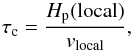 (A.1)where Hp(local) is the pressure scale height and vlocal is the convective velocity, both quantities computed at a distance of 0.95Hp(base cz) above the base of the outer convective zone, where Hp(base cz) is the pressure scale height at the base of the convection zone.
Noyes et al. (1984) derived for that particular value of αMLT a polynomial fit for the turnover time as a function of (B − V). The fit is given by the expression  (A.2)where x = 1.0 − (B − V) and τc is given in days.
Once τc is computed, and provided is known, Noyes et al. (1984) give the expression  (A.3)which allows a direct estimation of Prot; y is defined as
  .
.
The determination of Prot from the Rossby number and is valid if 0.4 < (B − V) < 1.4 and  . Similar quantitative relationships can be found in the paper by Mamajek & Hillenbrand (2008).
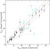 |
Fig. A.1 Rotation periods estimated according to the formalism described in this Appendix, plotted against the rotation periods for a sample of FGK stars with known values for Prot. Black symbols correspond to stars from Noyes et al. (1984) and cyan symbols to stars from Suárez Mascareño et al. (2015). The dashed lines mark the interval ± 5 days with respect to the diagonal. See text for details. |
In order to test the validity of these relationships when computing Prot for the stars analysed in this paper, we have taken the sample of 39 FGK stars given by Noyes et al. (1984) and 19 FGK stars by Suárez Mascareño et al. (2015), as well as the Sun, for which the rotation period are known by rotational modulation (first set) and time-series high-resolution spectroscopy (second set). Figure A.1 shows the comparison between the observed rotation periods and the rotation periods estimated following the formalism described above; the Noyes et al. sample is plotted in black and the Suárez-Macareño et al. sample is plotted in light blue. The uncertainties in both (B − V) and have been taken into account when available. Noyes et al. (1984) do not give any uncertainties in the observed periods or in , so we have assumed  . It can be seen that the agreement is fairly good, in particular for the Noyes et al. sample. Only two objects, namely HD 25171 and HD 40307, are clear outliers; therefore, we can consider the values of Prot computed for the DUNES_DB stars following this method, and shown in Table C.2 to be reliable.
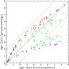 |
Fig. A.2 Ages for the DUNES_DU and DUNES_DB (d ≤ 20 pc) samples estimated by gyrochronology plotted against the chromospheric ages. F, G, and K stars are plotted in violet, green, and red, respectively. The dashed lines mark the interval ± 2 Gyr with respect to the diagonal. |
Concerning the ages, all the expressions were extracted from the paper by Mamajek & Hillenbrand (2008). Assuming that Prot is known, Eqs. (12)−(14) with the revised gyrochronology parameters a, b, c, and n in their Table 10 were used to derive the gyrochronology age (in Myr) ![Mathematical equation: \appendix \setcounter{section}{1} \begin{equation} t_{\rm~Gyro} = \left(\frac{P_{\rm rot}}{a\,[(B-V)-c]^b}\right)^{1/n} , \end{equation}](/articles/aa/full_html/2016/09/aa28329-16/aa28329-16-eq224.png) (A.4)
(A.4)
whereas expression (A.3) was used to estimate the chromospheric age  (A.5)
(A.5)
where tHK is the age in years. The gyrochronology expression is valid for B − V> 0.495 and the fit to estimate tHK is only appropriate for  . Figure A.2 shows a comparison between the ages of the whole DUNES_DU plus DUNES_DB samples estimated using both approaches; obviously, only the stars for which both ages could be estimated are included in the graph. The discrepancies between the ages are clear, the differences being more pronounced for earlier spectral types.
The caveats involving the determination of ages are well known, but its detailed discussion are beyond the scope
of this paper (details can be found in e.g. Barnes 2007; Mamajek & Hillenbrand 2008; Soderblom 2010; Epstein & Pinsonneault 2014; Meibom et al. 2015 and references therein). The bottom line of this analysis is that the rotation periods establish a reasonable evolutionary proxy for FGK stars, in the sense that the older the star the longer the rotation period, whereas the assignation of an specific age valid in a time span of the order of Gyr has to be taken with caution.
Appendix B: Spectral energy distributions
In this Appendix the SEDs of the excess, dubious, and non-excess sources are shown.
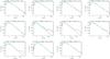 |
Fig. B.1 SEDs of the FGK DUNES_DB stars (d ≤ 20 pc) with excesses. |
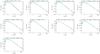 |
Fig. B.2 SEDs of the FGK DUNES_DB stars (d ≤ 20 pc) showing apparent excesses but considered dubious. |
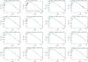 |
Fig. B.3 SEDs of the FGK DUNES_DB stars (d ≤ 20 pc) without excesses. |
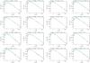 |
Fig. B.3 continued. |
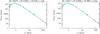 |
Fig. B.3 continued. |
Appendix C: Additional material
Subsamples of DUNES_DB stars with d ≤ 15 pc and 15 pc <d ≤ 20 pc.
Parameters of the DUNES_DB stars with d ≤ 15 pc and 15 pc <d ≤ 20 pc.
Multiplicity and planetary companions of the DUNES_DB stars with d ≤ 20 pc.
DUNES_DB stars with d ≤ 20 pc: Johnson V, B − V, Cousins V − I, and Strömgren photometry.
DUNES_DB stars with d ≤ 20 pc: 2MASS JHKs and ancillary Johnson JHKLL′M photometry.
DUNES_DB stars with d ≤ 20 pc: AKARI 9 and 18 μm fluxes and WISE W1, W3, and W4 photometry.
DUNES_DB stars with d ≤ 20 pc: IRAS 12, 25, 60 μm and Spitzer/MIPS 24 and 70 μm fluxes.
OBSIDs for the DUNES_DB stars with d ≤ 20 pc.
PACS flux densities for the DUNES_DB stars with d ≤ 15 pc and 15 pc <d ≤ 20 pc.
All Tables
Black-body dust temperatures and fractional dust luminosities for the DUNES_DB stars with excesses.
Summary of stars per spectral type in the DUNES_DU and DUNES_DB samples and frequency of excesses.
DUNES_DB stars with d ≤ 20 pc: Johnson V, B − V, Cousins V − I, and Strömgren photometry.
DUNES_DB stars with d ≤ 20 pc: 2MASS JHKs and ancillary Johnson JHKLL′M photometry.
DUNES_DB stars with d ≤ 20 pc: AKARI 9 and 18 μm fluxes and WISE W1, W3, and W4 photometry.
DUNES_DB stars with d ≤ 20 pc: IRAS 12, 25, 60 μm and Spitzer/MIPS 24 and 70 μm fluxes.
PACS flux densities for the DUNES_DB stars with d ≤ 15 pc and 15 pc <d ≤ 20 pc.
All Figures
|
Fig. 1 HR diagram for the FGK stars of the DUNES sample observed by the DEBRIS team (DUNES_DB). The colour codes following the Hipparcos spectral types are F stars (violet), G stars (green), and K stars (red). Solid circles represent FGK stars closer than 20 pc; empty triangles are FGK stars further away. The two red dots at the bottom right of the diagram are two stars classified as K5 in the Hipparcos catalogue, but their colours correspond to M stars. See text for details. |
| In the text | |
|
Fig. 2 Cumulative distributions (normalized) for the DUNES samples with d ≤ 15 pc (105 stars, red) and d ≤ 20 pc (177 stars, blue) and the FGK stars in the Hipparcos catalogue with d ≤ 15 pc (154 stars, grey), all plotted against stellar mass. A Salpeter law with exponent −2.35 has been normalized to the distributions. See text for details. |
| In the text | |
|
Fig. 3 Cumulative number of F, G, and K stars (luminosity classes V and IV−I) in the Hipparcos catalogue (red) and in the DUNES sample (black), both at d ≤ 15 pc. |
| In the text | |
|
Fig. 4 Upper limits of the fractional luminosity of the dust for the non-excess sources of the DUNES_DB (crosses) and the DUNES_DU (dots) samples within 20 pc, plotted against the effective temperature, distance, and stellar flux at 100 μm. Violet, green, and red represent F, G, and K stars. See text for details. |
| In the text | |
|
Fig. 5 Plotted in black, the histogram of the 100 μm significance χ100 for the non-excess sources of the merged DUNES_DU and DUNES_DB samples with d ≤ 20 pc (dubious sources of both samples are not included). A Gaussian with σ = 1.40, the standard deviation of the χ100 values for these sources, is plotted in blue. In cyan, we show a Gaussian with σ = 1.02, corresponding to the subsample of non-excess sources with −2.0 <χ100< 2.0. In red, the distribution of χ100 for the excess sources is also displayed. This figure is an extension of Fig. 6 in E13. See text for details. |
| In the text | |
|
Fig. 6 Cumulative distributions of the frequency of excesses obtained in this work (black) and those obtained from Spitzer/MIPS results Bryden et al. (2006; cyan), both plotted against fractional dust luminosity. The green straight line is a fit to the values of the frequencies at the less steep part of our cumulative distribution. The extrapolation down to 10-7, the current estimate of the Kuiper-belt fractional luminosity, gives a prediction for the incidence rate of excesses of ~0.25. The extrapolation from a straight line, plotted in red, fitted to the steeper part of the distribution, that mimics the MIPS results, gives a higher prediction ~0.35. The prediction from the Bryden et al. (2006) distribution, from the blue straight-line fit, is ~0.32. See text for details. |
| In the text | |
|
Fig. 7 Projected binary separation plotted against disc radius for excess sources in those stars catalogued as binaries. Red and blue symbols represent objects studied in this work and in E13, respectively. Squares and diamonds are confirmed or dubious excesses. Filled and open symbols represent the value of RBB and Rdust (see text for details). The inverted triangles at the bottom represent the binary HIP 77257 for which the separation is not known. |
| In the text | |
|
Fig. 8 Fractional dust luminosities Ldust/L∗ for the DUNES_DU and DUNES_DB stars with excesses (squares) and d ≤ 20 pc (Table 14 in E13 and Table 2 in this work), and upper limits for the non-excess sources (crosses), all of them plotted against metallicity, [Fe/H]. F, G, and K stars are plotted in violet, green, and red. The short-dashed vertical line marks the mean metal abundance of the whole sample, [Fe/H] = −0.11, whereas the long-dashed line marks the median, [Fe/H] = −0.095. The horizontal lines mark the means (solid) of the fractional luminosities for the debris discs of stars showing excess, with [Fe / H] ≤ −0.11 and >−0.11, and plus and minus their standard errors (dotted), defined as σ/ |
| In the text | |
|
Fig. 9 Diagram of |
| In the text | |
|
Fig. 10 Diagram of Prot – (B − V) showing the stars of the full DUNES sample with d ≤ 20 pc (cyan squares). As in Fig. 9 the stars identified as having far-infrared excesses are plotted as diamonds with a size proportional to the value of the fractional dust luminosity. Superimposed are five gyrochrones computed following Mamajek & Hillenbrand (2008; see Appendix A in this work). |
| In the text | |
|
Fig. 11 Diagram of Ldust/L∗ – Tdust showing the position of the 36 stars, out of the 177 in the DUNES sample within 20 pc, for which an excess has been detected at far-IR wavelengths. F, G, and K stars are plotted in violet, green, and red. The detection limits for a G5 V star at 20 pc for PACS 100 μm and MIPS 70 μm are also included. |
| In the text | |
|
Fig. A.1 Rotation periods estimated according to the formalism described in this Appendix, plotted against the rotation periods for a sample of FGK stars with known values for Prot. Black symbols correspond to stars from Noyes et al. (1984) and cyan symbols to stars from Suárez Mascareño et al. (2015). The dashed lines mark the interval ± 5 days with respect to the diagonal. See text for details. |
| In the text | |
|
Fig. A.2 Ages for the DUNES_DU and DUNES_DB (d ≤ 20 pc) samples estimated by gyrochronology plotted against the chromospheric ages. F, G, and K stars are plotted in violet, green, and red, respectively. The dashed lines mark the interval ± 2 Gyr with respect to the diagonal. |
| In the text | |
|
Fig. B.1 SEDs of the FGK DUNES_DB stars (d ≤ 20 pc) with excesses. |
| In the text | |
|
Fig. B.2 SEDs of the FGK DUNES_DB stars (d ≤ 20 pc) showing apparent excesses but considered dubious. |
| In the text | |
|
Fig. B.3 SEDs of the FGK DUNES_DB stars (d ≤ 20 pc) without excesses. |
| In the text | |
|
Fig. B.3 continued. |
| In the text | |
|
Fig. B.3 continued. |
| In the text | |
Current usage metrics show cumulative count of Article Views (full-text article views including HTML views, PDF and ePub downloads, according to the available data) and Abstracts Views on Vision4Press platform.
Data correspond to usage on the plateform after 2015. The current usage metrics is available 48-96 hours after online publication and is updated daily on week days.
Initial download of the metrics may take a while.