| Issue |
A&A
Volume 592, August 2016
|
|
|---|---|---|
| Article Number | A100 | |
| Number of page(s) | 9 | |
| Section | The Sun | |
| DOI | https://doi.org/10.1051/0004-6361/201628889 | |
| Published online | 08 August 2016 | |
Reconnection brightenings in the quiet solar photosphere⋆
1 Institute of Theoretical Astrophysics, University of Oslo, PO Box 1029 Blindern, 0315 Oslo, Norway
e-mail: This email address is being protected from spambots. You need JavaScript enabled to view it.
2 Lingezicht Astrophysics, ’t Oosteneind 9, 4158 CA Deil, The Netherlands
Received: 10 May 2016
Accepted: 11 June 2016
Abstract
We describe a new quiet-Sun phenomenon which we call quiet-Sun Ellerman-like brightenings (QSEB). QSEBs are similar to Ellerman bombs (EB) in some respects but differ significantly in others. EBs are transient brightenings of the wings of the Balmer Hα line that mark strong-field photospheric reconnection in complex active regions. QSEBs are similar but smaller and less intense Balmer-wing brightenings that occur in quiet areas away from active regions. In the Hα wing, we measure typical lengths of less than 0.5 arcsec, widths of 0.23 arcsec, and lifetimes of less than a minute. We discovered them using high-quality Hα imaging spectrometry from the Swedish 1-m Solar Telescope (SST) and show that, in lesser-quality data, they cannot be distinguished from more ubiquitous facular brightenings, nor in the UV diagnostics currently available from space platforms. We add evidence from concurrent SST spectropolarimetry that QSEBs also mark photospheric reconnection events, but in quiet regions on the solar surface.
Key words: Sun: photosphere / Sun: chromosphere / Sun: magnetic fields / Sun: faculae, plages / Sun: activity
The movies are available in electronic form at http://www.aanda.org
© ESO, 2016
1. Introduction
Reconnection brightenings in the solar photosphere are well-known in their manifestation as Ellerman bombs (EB). EBs are small but intense brightenings of the extended wings of the hydrogen Balmer-α line at 6563 Å (henceforth Hα) that occur intermittently in complex bipolar active regions and mark magnetic reconnection in the low solar atmosphere.
Here we report the discovery of similar, but weaker, Hα-wing brightenings in quiet solar areas away from active regions. We call them quiet-Sun Ellerman-like brightenings (QSEB) and show evidence that also these mark magnetic reconnection in the low solar atmosphere.
Ellerman (1917) described his “hydrogen bombs” so well that in their review Bray & Loughhead (1974) concluded that the subsequent EB literature at the time did not add much to his description. More recently this situation changed, first with high-quality observations from the Flare Genesis balloon telescope (Bernasconi et al. 1999; Georgoulis et al. 2002; Schmieder et al. 2004; Pariat et al. 2004, 2006) and then with yet better observations from the Swedish 1-m Solar Telescope (SST, Scharmer et al. 2003; Watanabe et al. 2011, henceforth Paper I; Vissers et al. 2013, henceforth Paper II; Vissers et al. 2015, henceforth Paper III; Rutten et al. 2015, henceforth Paper IV; Nelson et al. 2015; Reid et al. 2015, 2016).
These studies have firmly established that EBs result from strong-field reconnection taking place in the photosphere. They contain so much heating that they become visible even in UV lines normally arising from the transition region (Paper III; Tian et al. 2016).
In observing EBs near solar disk center it is non-trivial to distinguish them from ubiquitous strong-field magnetic concentrations (MC) that are abundant in active regions and constitute plage and network elsewhere. These also brighten the Hα wings (Leenaarts et al. 2006b). Many papers in the EB literature have confused these MC brightenings with EB brightenings (so-called pseudo EBs, Rutten et al. 2013). Therefore, in Papers I–IV our strategy has been to observe EBs well away from disk center. In slanted-view Hα-wing images EBs appear as flames with characteristic morphology: upright, tall (1 – 2 Mm), rapidly flickering on fast timescales (seconds), and often with their feet traveling at high speed (1 km s-1) along network lanes filled with MCs and then occurring repetitively in quick succession (Paper I). These signature properties became our way to distinguish EBs from MCs in high-resolution imaging spectrometry with the SST (Papers II–IV).
We employed the same strategy of limbward flame detection when we decided to search for EB-like phenomena in quiet areas outside active regions. This search was inspired by numerical simulations presented by S. Danilovic at a recent ISSI meeting in Bern. In her simulations, reconnection in the quiet low photosphere produced small flames in synthesized Hα-wing images that appear rather like observed EBs, although smaller. We found that such small EB-like flames indeed also occur outside active regions on the actual solar surface, but that their detection is only possible at the very best seeing at the SST and even then requires the utmost of the advanced adaptive optics and image restoration developed at this telescope.
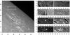 |
Fig. 1 Examples of EBs and QSEBs in dataset 2 which targeted active region AR 11778 near the limb. The SST field is rotated over −59 deg from solar (X,Y). The full-field overview at left was taken with the blue (λ = 3953.7 Å) wide-band (FWHM 10 Å) camera. The axis divisions are arcsec from the lower-left corner. The four regions of interest A–D are shown enlarged as Hα-wing and blue wide-band cutout pairs at right, with corresponding arcsec coordinates. Regions A and B are in quiet areas, regions C and D sample the active region. Ellerman features are visible as bright flames in the Hα wings, respectively as smaller and weaker QSEBs in A and B and as larger and brighter EBs in C and D. Their relative brightness enhancements can be judged from the darkness of the surrounding granulation because each cutout panel is independently greyscaled. They are invisible in the blue wide-band images at right, in contrast to facular striations which are visible in both diagnostics, although appearing darker in Hα from the greyscaling needed to accommodate the bright Ellerman flames. |
Overview of the CRISP datasets analyzed in this study.
This decisive need for highest image quality results from the likelihood of confusion between QSEBs and MCs, similar to the confusion between EBs and MCs nearer disk center. While MCs constituting network appear as roundish Hα-wing brightness features in top-down viewing, they become elongated towards the limb in becoming faculae. This is because, in top-down viewing, the Hα-wing brightening is from subsurface hot-wall emission (Spruit 1976; Leenaarts et al. 2006b), whereas in limbward observation relatively empty fluxtubes are mapped by permitting deeper slanted viewing into hot granule interiors behind them (cartoon in Fig. 7 of Rutten 1999; simulations in Keller et al. 2004 and Carlsson et al. 2004). The resulting facular striations have elongated upright stalk appearance and so may masquerade as small reconnection flames (pseudo QSEBs). However, at the image quality of the SST during the best La Palma seeing, definite distinction can be made, as we demonstrate below.
The next section presents the observations and their reduction. We then present the results and end the paper with discussion and conclusion.
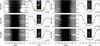 |
Fig. 2 Sample λ−t diagrams and spectral profiles of Ellerman features in Hα at the observing angles specified at lower-right in the profile plots. Panel pair a) is from dataset 2, b) and c) from 1, d) from 8, e) from 7, f) from 6. Pair a) shows an active-region EB for comparison, the one at the bottom at (x,y) ≈ (29″,15″) in Hα-panel D of Fig. 1. The other pairs show QSEBs. Each λ−t image is greyscaled between 0.3 and 1.5 times the Hα far wing intensity. The Ellerman feature occurs at time 0. The profiles are normalized to the outer-wing intensity of the time-averaged profile (dashed) of an area close to the Ellerman feature. Note the scale difference for profile graph a). The orange profile added to a) is from the facular brightening visible at the top of the small inset image. The red pluses in the blue wing of each feature profile (solid) specify the spectral sampling of the small image insets (size 2.3 by 4.6 arcsec) in which central red dots mark the location of the spectral sampling. In pair a) the location of the facular sampling is also marked in the inset (easier seen per zoom-in with a pdf viewer). The limb direction is upward. |
2. Observations and data reduction
Over the past decade, the Oslo group has collected over 70 high-quality datasets with the SST. From these we have selected the very best in our search for limbward Ellerman-like phenomena in quiet areas. The ones from which we present results here are from the 2013, 2014, and 2015 observing seasons and are detailed in Table 1. They targeted quiet areas, except for the second dataset in which the field of view contained an active region (Fig. 1). Datasets 1–3 and 5 included the limb in the field of view (see μ specification in the fourth column).
These data were obtained with the CRISP Fabry-Pérot interferometer at the SST (Scharmer et al. 2008). It provides imaging spectroscopy in Hα with transmission profile FWHM 66 mÅ, image scale 0.̋058 per pixel, and a field of view of about 60′′× 60′′. Some datasets also contain CRISP spectral imaging in Ca ii 8542 Å with FWHM 107 mÅ and imaging spectropolarimetry in Fe i 6173 Å with FWHM 51 mÅ.
QSEBs are small and can only be identified in SST data that reach the telescope diffraction limit λ/D = 0.̋14 at 6563 Å. Imaging of this quality requires not only a superb telescope and extremely stable atmospheric conditions, but also high-order adaptive optics, at the SST employing an 85-electrode deformable mirror, and advanced subsequent image restoration, in our case multi-object multi-frame blind deconvolution (MOMFBD, van Noort et al. 2005). In its application here we used eight exposures per CRISP spectral line position (or spectropolarimetric state for Fe i 6173 Å). We followed the extensive CRISPRED data-reduction pipeline (de la Cruz Rodríguez et al. 2015) including time-dependent derotation, coalignment and destretching.
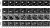 |
Fig. 3 Temporal evolution of Ellerman features at 1-s cadence in Hα wide-band (FWHM = 4.9 Å) image sequences. Each row of image cutouts shows selected samples with identical greyscaling per panel. The limb direction is upward. Row a) contains an active-region EB from dataset 2 (close to the limb, cutout C in Fig. 1). The other rows show QSEBs in quiet areas in yet smaller cutouts from datasets 5 b), close to the limb and 4 c) and d), μ = 0.56. The time labels specify duration from the start of each observation. Corresponding animations of this figure are available online. |
For the Hα-only CRISP datasets 1–6 we also processed the Hα prefilter data (FWHM 4.9 Å) in parallel in order to obtain simultaneous sequences sampling the low photosphere at a cadence of only 1 s. These permit to study fast temporal evolution within QSEBs similarly to the EB analysis in Paper I (Fig. 3).
For datasets 1 and 2 we include imaging with the SST blue beam that consist of MOMFBD-restored filtergrams in Ca ii H 3969 Å (FWHM 1.1 Å), Ca ii K 3934 Å (FWHM 1.5 Å), and with a wider “blue” passband (FWHM 10 Å) at λ = 3954 Å between the Ca ii H and K lines which shows the lower photosphere. The image scale for these is 0.̋034; the field of view slightly exceeds the CRISP imaging. They were recorded at 10.8 frames per second with 9.5 ms exposure and MOMFBD-restored to yield sequences at the cadence of the cotemporal CRISP data (3.3 and 8.6 s, see Table 1).
To check for QSEB signatures in hotter diagnostics sampling the upper chromosphere, transition region and corona for some datasets we also coaligned cotemporal observations from the Interface Region Imaging Spectrograph (IRIS, De Pontieu et al. 2014) and from the Atmospheric Imaging Assembly (AIA, Lemen et al. 2012) onboard the Solar Dynamics Observatory (SDO, Pesnell et al. 2012), as specified in Table 1.
From IRIS, we analyzed slit-jaw images (SJI) in the 1400 and 1330 Å channels (dominated by Si iv and C ii lines, respectively, both filters have FWHM 55 Å), and the 2796 Å channel containing Mg ii k in its FWHM 4 Å passband. For datasets 7–9 the slit-jaw data had 12 s cadence, 2 s exposure time, and spatial binning over 0.̋33 pixels. The alignment to the SST data was done through cross-correlation of the SJI 2796 Å images to the CRISP images in the Ca ii 8542 Å wing. In quiet solar areas they show very similar scenes. The accuracy of this alignment is about the IRIS pixel size. Dataset 3 has only SJI 1400 and 2796 Å at 19 s cadence, 8 s exposure time and no spatial binning (0.̋17 pixels). For this limb dataset, alignment to the SST data was done through cross-correlation of the on-disk part of the SJI 2796 Å and Ca ii H images.
The alignment of the AIA data, which have an image scale of 0.̋6 per pixel, was done for dataset 3 through cross-correlation of AIA 1600 Å images to Ca ii H images, for dataset 9 by aligning continuum images from the Helioseismic and Magnetic Imager (HMI, Schou et al. 2012) to CRISP Hα wing images, and for the other datasets by aligning HMI continuum images to CRISP Hα prefilter images.
For our data searches and our successful identifications of QSEBs we made extensive use of the CRISPEX imaging spectroscopy viewer of Vissers & Rouppe van der Voort (2012), a widget-based IDL tool for efficient inspection and analysis of multi-dimensional spectral-imaging data. It is available in the SolarSoft library as part of the IRIS package.
3. Results
Morphology. The defining appearance and morphology of QSEBs as small bright Hα-wing flames is illustrated in Fig. 1, including comparison with larger and brighter EB flames. The field of view of this dataset (nr. 2) is shown at left and includes a young emerging active region close to the limb as well as extended quiet areas. The righthand panels enlarge two cutouts in quiet areas (A and B) and two comparison ones in the active region (C and D).
The Hα red-wing images for C and D contain prominent EBs. They appear as upright flames quite similar to the EBs in Paper I, with the tallest in C nearly reaching 1.̋5 (1.1 Mm) in length and adhering to the remark by Ellerman (1917) that his bombs typically occur between spots in complex developing active regions.
The blue wide-band images at right do not show the EBs in C and D but instead bright faculae bordering granular “hills” seen from aside (Keller et al. 2004; Carlsson et al. 2004). All faculae are also visible in the Hα-wing images, in which their contrast over the granulation is actually larger (see last panels of Fig. 5), but here they appear less conspicuous because the greyscale is stretched to include the far brighter EBs. The marked differences in contrast and morphology confirm that EBs are distinct from facular striations, even though also these appear elongated and generally upright in the limbward projection.
The quiet regions in A and B show QSEBs in the inner blue Hα wing as small elongated brightenings. They are comparable to the EBs in C and D but less tall and less bright. Their invisibility in the blue companion images at right demonstrates that these quiet-Sun features are not faculae, just as for the active-region EBs in C and D. The tallest example is the QSEB in panel B. It is visible through a forest of dark spicular features in the foreground which are rapid blue-shifted excursions (RBE, Rouppe van der Voort et al. 2009). This QSEB has length 0.̋6 (0.4 Mm) and width below 0.̋25 (0.18 Mm). Panel A contains multiple smaller QSEBs, with the smallest hardly elongated and reaching only 0.̋29 (0.21 Mm) extent, marginally taller than its width of 0.̋21 (0.15 Mm). This sample is closer to the limb than B, causing darker granulation background at similar QSEB brightness.
From similar measurements for a sample of 24 QSEBs in dataset 1 and 21 QSEBs in dataset 2 we conclude that QSEBs typically have lengths below 0.̋5 (0.36 Mm) and widths of only 0.̋23 (0.17 Mm). We selected these limb datasets for these measurements on the assumption that QSEBs generally stand upright, so that near-limb viewing effectively gives a side view minimizing projection uncertainty in the length measurement. The typical lifetimes for these QSEBs was measured to be less than a minute.
Spectral detail. Figure 2 continues our presentation of QSEBs by showing spectral evolution and detailed line profiles of Hα for multiple examples.
The first pair of panels is not a QSEB but an active-region EB serving as comparative reference. Its Hα profile has enhanced wings that reach maximum at −1.2 Å from line center and double the far-wing intensity of the local reference spectrum. Near line center, the EB spectral profile is as dark as the reference due to obscuration by dark chromospheric fibrils overlying the photospheric reconnection site below the canopy (Paper I). The spectral evolution slice at left shows that this EB was preceded by multiple such flarings during the preceding minutes, a common EB characteristic that was already noted by Ellerman (1917).
The orange profile in the graph is not for an Ellerman feature but from the facular MC at the top of the small image inset. It demonstrates that faculae brighten the Hα wings less than EBs do.
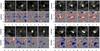 |
Fig. 4 Four examples of magnetic field evolution around QSEBs. The four upper panels per sequence show Hα wing image cutouts at Δλ = −1 Å, the four lower panels corresponding Stokes V/Icont maps obtained from CRISP spectropolarimetry in Fe i 6173 Å. These are averages over 6 wing positions at Δλ = ± 0.150, ± 0.105, and ± 0.070 Å from line center. Signals below 3σnoise are put to 0 in the greyscaling, positive polarity is white with red contours, negative polarity is black with blue contours. The contour levels are at 0.2, 0.5, 1, and 2% polarization. The yellow cross at the center of each panel serves to guide inspection. a) and c) are from dataset 7 (μ = 0.73), b) and d) from dataset 8 (μ = 0.64). Animations of this figure are available in the on-line material. (Online movie.) |
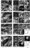 |
Fig. 5 Three QSEBs and one pseudo-QSEB in Hα line center over a fairly wide field of view (first column) and in smaller image cutouts clockwise sampling the blue wing of Hα, the wide-band continuum around Hα, AIA 1600 Å or Ca ii 8542 Å wing, AIA 1700 Å, IRIS slit-jaw 1400 Å or 1330 Å, and the core of Fe i 6173 Å. The dotted frame in the first column specifies the smaller cutouts at right. The axis units are arcsec from the feature at (0,0). The first row is from dataset 8 (μ = 0.64), the others are from dataset 7 (μ = 0.73). The QSEB in row c) is the same as in Fig. 2e; for this one the AIA 1700 image is replaced by a Ca ii 8542 Å profile plot. White horizontal markers are added to guide the eye: the QSEB visible in the Hα wing is slightly above the small bright point also visible in the other SST diagnostics (marked with the lower left marker). Row d) shows a pseudo-QSEB, i.e., facular striations. The AIA 1700 Å image is replaced by a plot of the Hα profile of the facula at image center (solid profile without crosses). The other profiles (with crosses and dashed) are for the QSEB and its reference spectrum in row c), copied from Fig. 2e. |
Panels pairs b−f of Fig. 2 show example QSEBs ordered over increasing viewing angle μ. They show similarly enhanced Hα wings, but with lower contrast than the EB in pair a. However, some yet reach maximum Hα-wing intensity equal to or exceeding the value of 1.5 times the reference far-wing intensity which was defined as intensity threshold for automated EB detection in Paper II. But even when QSEBs reach this EB threshold we would not designate them as EBs since they are not in active regions as described by Ellerman (1917). In addition, they have discordant spectral visibilities described below.
Examples panels b and c stay below 1.5 and have wing intensities comparable to the orange facular profile in panel a. However, their spectral evolutions in the λ−t diagrams show brief lifetimes, below a minute, while faculae evolve at granular time scales and last multiple minutes. We also note that faculae as bright as the orange profile in panel a are mostly found in active-region plage and strong network, rarely in quiet-Sun areas. Furthermore, the QSEB spectral profiles are different from faculae: they taper off towards larger offset beyond their maximum at about −1 Å, while the facular profile keeps rising towards the blue limit of the CRISP scan (this can only be inspected for the blue Hα wing; the red wing decreases for both QSEBs and faculae from line blends around + 1.3 Å). Indeed, faculae also brighten the continuum while QSEBs do not (Fig. 5).
Examples panels e and f are from fields nearer disk center and indeed appear more roundish than flame-like. Their wing brightness reaching 1.5 is the main discriminator from faculae.
In all profile graphs the line core of the feature duplicates the core of the reference profile. The reason is that in all areas the Hα core originates in obscuring overlying fibrils that together constitute the chromospheric canopy. Examples are shown in the first column of Fig. 5 (in particular, the Hα core image of the QSEB from panel e is shown in Fig. 5c).
Note that none of these QSEBs showed repetitive flaring over the course of minutes as was the case for the EB in pair a and happens often for EBs.
Temporal behavior. Figure 3 illustrates temporal behavior of an EB (top row) and multiple QSEBs (other rows). The images are taken with a wide-band Hα filter and are part of several time series that have a temporal cadence of 1 s. Figure 3 shows eight selected images from each time series, the corresponding animations are available online. The high cadence reveals fast dynamical evolution in these events, similar to the EBs in similar Hα wide-band data in Paper I.
The 21-min EB movie corresponding to the top row of Fig. 3 shows complex dynamical evolution of EBs at several sites in this area. The site in the top left quadrant has EBs present throughout the full movie duration. There seem to be both upflows and downflows associated with these EBs, with apparent downflows mostly in the bottom part and apparent upflows mostly in the top.
The three QSEB movies show events that are less tall but display similar morphology and similar fast changes with time, faster than the changes in the background granulation. The darker background of the EB images illustrates that its brightness is larger than the QSEB brightnesses. During the ~9 min duration of the QSEB sequence b, one can distinguish at least six different QSEB events. Some show comparable up and downflows as in the EB sequence. The lower two sequences are further from the limb; the QSEBs show less clear upright-flame morphology than in the top QSEB sequence. Sequence c shows two separate, short-lived QSEB events while the bottom sequence shows a QSEB with signs of the fast repetitive flaring that is so clearly present in some of the EB events.
Magnetic surroundings. Figure 4 compares QSEB evolution for four cases with the magnetic environment obtained from Fe i 6173 Å polarimetry. In each case the topography is bipolar, with the “pepper-and-salt” patterning that is characteristic of quiet areas. In all, the QSEB originates close to one fairly strong patch with comparable opposite polarity patches not far away. Case a suggests cancellation of negative polarity against opposite polarity at the QSEB site; both polarities diminish in presence. Case c similarly shows sizable reduction of both polarities with time. Case d shows reduction of the relatively strong negative-polarity patch to the lower right of the QSEB.
Visibility in other diagnostics. Figure 5 completes our presentation of the QSEB phenomenon by comparing their visibility in Hα with their visibility in other spectral diagnostics, and also comparing QSEB appearance with facular striations (“pseudo-QSEBs”).
Cases a and b show QSEBs without signature in the optical continuum, nor in Fe i 6173 Å and in AIA and IRIS UV imaging.
Case c suggests that there is a tiny continuum bright point at the foot of the QSEB flame with corresponding brightening of Ca ii 8542 Å and Fe i 6173 Å. The Ca ii 8542 Å profile also shows higher wing intensities than in the reference spectrum, but the increase remains below the minimum 140% wing brightening threshold defined for EBs in Paper II; the brightening in the image cutout is indeed less than for other magnetic concentrations nearby. Similarly, Ca ii 8542 Å wing for case b shows a small bright point at the site of the QSEB but not nearly at the high contrast as in the Hα wing. The Ca ii 8542 Å wings stay below the 120% as compared to the reference (not shown for this case). Detailed CRISPEX inspection of Ca ii 8542 Å behavior at the sites of other QSEBs confirmed that they do not show up as noticeable features in this line.
Case d serves to compare facular brightening with QSEB brightening. The facular striation morphology is identical between the Hα wing, the continuum, the core of Fe i 6173 Å, and even in the UV images at their much coarser resolution. One might expect that the small size of QSEBs makes them invisible at the 1.2 arcsec AIA resolution, but this example and more in general the good visibility of MCs in the AIA UV channels suggests an intrinsic lack of UV continuum brightening for QSEBs.
The Hα profile indeed suggests continuation into continuum brightening beyond the CRISP spectral sampling extent.
4. Discussion
Small reconnection events. QSEBs have similar bright-flame appearance in the Hα wings as EBs (Figs. 1–3), but they occur in quiet areas instead of active regions (Figs. 1, 3–5), they are less bright and less tall (Figs. 1–3), and they differ significantly in their spectral visibilities (Fig. 5). Nevertheless, they probably also mark small-scale magnetic reconnection in the photosphere (Fig. 4).
It seems that there is an extended range of small reconnection events taking place in the low solar atmosphere, with variation in magnetic topography, amount of reconnection, released energy, and penetration into the higher atmosphere. At the top end there are small flaring active-region fibrils (FAF), very bright in AIA 1600 Å images, often producing “IRIS bombs”, and affecting the atmosphere above the chromospheric canopy (Pariat et al. 2009; Rutten et al. 2013; Peter et al. 2014; Paper III; Rutten 2016; Tian et al. 2016).
Next are EBs which are also limited to complex bipolar active regions but only rarely penetrate through the canopy (there are reports of accompanying surges but these are rare, see Georgoulis et al. 2002; Paper I; Paper II; Reid et al. 2015). Nevertheless, also the sub-canopy heating in EBs can be large enough to cause significant brightening of the UV IRIS lines (Paper III; Tian et al. 2016).
The QSEBs reported here represent a yet weaker member of this family occurring in quiet areas and without signature at UV wavelengths.
Spectral visibilities. QSEBs share key spectral characteristics with EBs: they show up as intense wing brightenings of Hα without affecting the Hα core, they do not show up in the optical continuum, and they do not show up in neutral-atom lines, at least not in Fe i 6173 Å. However, they differ distinctly from EBs in other characteristics since they do not show up in the Ca ii 8542 Å line nor in the AIA and IRIS UV continua, whereas EBs and also MCs do show up in these diagnostics. In addition, EBs can show strong emission in UV “transition-region” lines including even Si iv (Paper III; Tian et al. 2016).
Let us first discuss MC visibilities. The most detailed analysis of MC “line gap” brightening of Fe i lines in top-down viewing is in Vitas et al. (2009); it results from enhanced Fe i ionization in low-density fluxtubes. MC brightenings as “G-band bright points” result similarly from CH dissociation (Rutten et al. 2001; Carlsson et al. 2004). MC brightening of the Hα wings also results from relatively low gas density but not by ionization but by less collisional damping (Leenaarts et al. 2006a, b).
The good MC visibility in UV continua results also from ionization of Fe i and the other neutral “electron donor” species since their bound-free edges dominate the UV continuous extinction in the upper photosphere. Hence, in top-down viewing the UV MC radiation originates much deeper than the height of formation suggested by standard one-dimensional non-magnetic solar atmosphere models. It is a misconception to attribute MC UV brightness to heating; it is also “hole-in-the-surface” radiation as in Spruit (1976). The observed morphology samples the low photosphere; indeed, near the center of the disk the UV bright points correspond closely to MCs in photospheric magnetograms, a useful property for coaligning HMI and AIA imagery also exploited here.
The same visibility mechanisms apply in slanted viewing towards the limb where MCs appear as faculae, again with MC tenuity causing fluxtube transparency in minority-stage lines and edges through ionization, in the Hα wings through less damping. The cutout images on bottom row d of Fig. 5 show this very well: the morphology of the facular striae is remarkably similar between these diagnostics.
EBs also show up in UV continua but much brighter than MCs (Paper II). The EB visibility analysis by Rutten (2016) suggests that they are so hot (over 10 000 K) that Balmer continuum extinction, which increases very steeply with temperature, exceeds the extinction of the metal edges and H−.
The QSEB visibilities represent an intermediate class. The absence of visibility in Fe i 6173 Å combined with their low-photosphere anchoring (shown by flame feet being located in intergranular lanes when viewed from aside, best seen in Fig. 3) suggests sufficient heating to ionize Fe i – but in gas that is denser than the surroundings, not more tenuous as is the case in MCs. Reconnection simulations as the one of Archontis & Hood (2009) indeed predict sizable density increase in such events.
The QSEB invisibility in the UV continua may then be explained by the gain in H− extinction from the density increase offsetting the loss of metal-edge extinction from ionization, but without getting as hot as EBs and therefore not passing into Balmer-continuum domination.
The lack of significant wing brightening in Ca ii 8542 Å suggests that the heating in QSEBs does not reach the heights where this line forms, whereas it does in EBs. It is therefore of interest to observe QSEBs also in the Na i D and Mg i b lines which form at intermediate heights (Paper IV; Rutten 2016).
EB visibilities already define a complex set of constraints that is hard to explain by classical static modeling and probably requires time-dependent non-equilibrium modeling (Rutten 2016). The same is likely the case for the QSEB visibilities reported here.
Temperatures. The extinction curves in Fig. 5 of Rutten (2016) together with the QSEB and EB visibilities suggest that both QSEBs and EBs form at high density (total hydrogen density about 1015 cm-3) but at temperatures around 8000 K in QSEBs, causing visibility in the Hα wings but invisibility in the Balmer continuum, and at temperatures above 10 000 K for EBs causing visibility also in the Balmer continuum and the IRIS lines.
Modeling. There have been Hα best-fit EB modeling efforts based on perturbing a standard model atmosphere in 1D or 2D geometry (Kitai 1983; Berlicki et al. 2010; Bello González et al. 2013; Berlicki & Heinzel 2014) that proposed EB temperatures below 10 000 K. These have been criticized for not being able to explain observed EB brightness in the IRIS lines (Paper III; Paper IV; Rutten 2016; Tian et al. 2016). We now suggest that these models may be more appropriate to describe QSEBs rather than EBs. The same may hold for the EB simulation efforts in Nelson et al. (2013) and Reid et al. (2015).
Energy release. Since all our observed QSEBs have Hα cores that are dominated by overlying chromospheric fibrils we cannot establish what the intrinsic Hα-core profiles of QSEBs are, just as is the case for EBs. The Hα opacity of these features must increase very much towards line center so that one may expect intrinsic profiles that are comparable to those of other very strong lines, in particular Mg ii k which has similar line-center extinction as Hα in the EB parameter range proposed by Rutten (2016). We may therefore expect a profile underneath the canopy resembling Mg ii k in shape: having high twin peaks with a central self-absorption dip from resonance scattering. The line core cannot be observed since blocked by the fibril canopy, but underneath that it represents a bright radiator.
Estimation of Hα radiation loss based on observed extended-wing emission excess and assuming optically thin line formation, as done recently for EBs by Reid et al. (2016), ignores this intrinsic core contribution and that the features are optically thick already in the observed Hα wing enhancements since EBs and QSEBs appear intransparent.
In our opinion, quantitative estimation of the radiation losses in these features first requires convincing duplication of their characteristics and spectral visibilities in a numerical MHD simulation, then detailed analysis of the radiation budget in such a simulation. However, since QSEBs and most EBs do not affect the chromospheric canopy nor the higher atmosphere, such evaluation seems unimportant in the context of chromospheric or coronal heating in general.
Reconnection scenario. The magnetogram sequences in Fig. 4 suggest reconnection as QSEB cause by showing complex bipolar field patterns with considerable evolutionary change. However, the topography is less clear-cut then for EBs which at the best seeing in SST magnetometry always mark cancelation of small patches of field that move fast into larger patches of opposite polarity (Paper II), usually at sites with fast and sheared streaming motions and correspondingly elongated granules. Even at the low AIA resolution fast movie playing of its 1700 Å sequences, which we have done for many emerging active regions, shows invariably that EBs occur at sites where MCs move together, usually with one (visible as a bright 1700 Å pixel) coming in fast from far away. For EBs in emerging active regions these characteristics suggest confirmation of the large-scale serpentine U-loop emergence scenario advocated by, e.g., Bernasconi et al. (2002), Pariat et al. (2004), Isobe et al. (2007), Archontis & Hood (2009), Pariat et al. (2009).
For QSEBs we may consider small-scale Omega-loop emergence with a mass-collecting and reconnecting “dipped” sag between the anchored opposite-polarity feet, as in cartoon models a in Fig. 12 of Georgoulis et al. (2002) and 2a in Fig. 17 of Watanabe et al. (2008). The major difference with EBs may be that in active-region serpentine emergence the mass drainage occurs over much larger loop lengths, feeding larger reconnection events.
Nomenclature. It has been suggested to us that we should not increase the taxonomic categories of solar features with yet another one. However, we feel that simply calling QSEBs “EBs in quiet areas” would be dangerously misleading. The EB literature contains many publications that mistook quiescent MCs for EBs. The risk that such misinterpretation affect QSEBs is even larger because they are intrinsically weaker than EBs. Their small-flame morphology may currently be rendered distinctively only by the SST. Also, Ellerman’s original description defines EBs as brilliant Hα-wing brightenings in complex active regions only. Furthermore, QSEBs differ intrinsically from EBs by not appearing as beyond-MC brightening in Ca ii 8542 Å nor showing up in UV continua. We therefore maintain our naming as QSEB, a new solar phenomenon.
5. Conclusion
We have described a new quiet-Sun phenomenon. It was not reported so far because it is very elusive: QSEBs can only be distinguished from near-limb facular striations in imaging spectroscopy that reaches the unsurpassed quality of the SST at the best La Palma seeing.
QSEBs probably originate from magnetic reconnection in the low photosphere and therefore promise to be valuable diagnostics to chart quiet-Sun field topography evolution.
The spectral visibilities of the QSEBs are complex. In some respects they are similar to those of active-region EBs (extended wing brightenings of Hα, no brightening of the optical continuum, no brightening of Fe i lines), but they differ significantly in other respects (no striking brightening of the wings of Ca ii 8542 Å, no brightening of the AIA 1600 and 1700 Å continua, no brightening in the IRIS UV slitjaw images).
The magnetic topography of the quiet areas where they occur suggests a reconnection scenario which differs from the one causing EBs in emerging active regions.
As is the case for EBs, advanced time-dependent radiation-MHD simulations seem required to understand the details of QSEB formation. Similarly to EBs (Rutten 2016), the synthesis of the various spectral diagnostics needed to reproduce and explain the diverse visibilities must probably account for non-equilibrium hydrogen ionization and recombination. The reward of such endeavor will be that the complex QSEB occurrence and visibility patterns will then provide sufficient constraints for definitive identification and analysis of the underlying reconnection processes.
Online material
Movie a of Fig. 3 Access Supplementary Material
Movie b of Fig. 3 Access Supplementary Material
Movie c of Fig. 3 Access Supplementary Material
Movie d of Fig. 3 Access Supplementary Material
Movie a of Fig. 4 Access Supplementary Material
Movie b of Fig. 4 Access Supplementary Material
Movie c of Fig. 4 Access Supplementary Material
Movie d of Fig. 4 Access Supplementary Material
Acknowledgments
The Swedish 1-m Solar Telescope is operated on the island of La Palma by the Institute for Solar Physics of Stockholm University in the Spanish Observatorio del Roque de los Muchachos of the Instituto de Astrofísica de Canarias. Our research has been partially funded by the Norwegian Research Council and by the ERC under the European Union’s Seventh Framework Programme (FP7/2007−2013) / ERC grant agreement nr. 291058. This work was initiated after discussions at the meeting “Solar UV bursts – a new insight to magnetic reconnection” at the International Space Science Institute (ISSI) in Bern. IRIS is a NASA small explorer mission developed and operated by LMSAL with mission operations executed at NASA Ames Research center and major contributions to downlink communications funded by ESA and the Norwegian Space Centre. We thank A. Drews, S. Jafarzadeh, T. Leifsen, T. Pereira, A. Sainz-Dalda, M. Szydlarski, R. Timmons, and P. Zacharias for their help with acquiring the observations. T. Pereira performed the alignment of the 2014 June 17 IRIS and AIA observations to the SST data. We made much use of NASA’s Astrophysics Data System Bibliographic Services.
References
- Archontis, V., & Hood, A. W. 2009, A&A, 508, 1469 [NASA ADS] [CrossRef] [EDP Sciences] [Google Scholar]
- BelloGonzález, N., Danilovic, S., & Kneer, F. 2013, A&A, 557, A102 [NASA ADS] [CrossRef] [EDP Sciences] [Google Scholar]
- Berlicki, A., & Heinzel, P. 2014, A&A, 567, A110 [NASA ADS] [CrossRef] [EDP Sciences] [Google Scholar]
- Berlicki, A., Heinzel, P., & Avrett, E. H. 2010, Mem. Soc. Astron. It., 81, 646 [NASA ADS] [Google Scholar]
- Bernasconi, P., Rust, D., Murphy, G., & Eaton, H. 1999, in High Resolution Solar Physics: Theory, Observations, and Techniques, eds. T. R. Rimmele, K. S. Balasubramaniam, & R. R. Radick, ASP Conf. Ser., 183, 279 [Google Scholar]
- Bernasconi, P. N., Rust, D. M., Georgoulis, M. K., & Labonte, B. J. 2002, Sol. Phys., 209, 119 [NASA ADS] [CrossRef] [Google Scholar]
- Bray, R. J., & Loughhead, R. E. 1974, The solar chromosphere (London: Chapman & Hall) [Google Scholar]
- Carlsson, M., Stein, R. F., Nordlund, Å., & Scharmer, G. B. 2004, ApJ, 610, L137 [NASA ADS] [CrossRef] [Google Scholar]
- de la Cruz Rodríguez, J., Löfdahl, M. G., Sütterlin, P., Hillberg, T., & Rouppe van der Voort, L. 2015, A&A, 573, A40 [NASA ADS] [CrossRef] [EDP Sciences] [Google Scholar]
- De Pontieu, B., Title, A. M., Lemen, J. R., et al. 2014, Sol. Phys., 289, 2733 [NASA ADS] [CrossRef] [Google Scholar]
- Ellerman, F. 1917, ApJ, 46, 298 [NASA ADS] [CrossRef] [Google Scholar]
- Georgoulis, M. K., Rust, D. M., Bernasconi, P. N., & Schmieder, B. 2002, ApJ, 575, 506 [NASA ADS] [CrossRef] [Google Scholar]
- Isobe, H., Tripathi, D., & Archontis, V. 2007, ApJ, 657, L53 [NASA ADS] [CrossRef] [Google Scholar]
- Keller, C. U., Schüssler, M., Vögler, A., & Zakharov, V. 2004, ApJ, 607, L59 [NASA ADS] [CrossRef] [Google Scholar]
- Kitai, R. 1983, Sol. Phys., 87, 135 [NASA ADS] [CrossRef] [Google Scholar]
- Leenaarts, J., Rutten, R. J., Carlsson, M., & Uitenbroek, H. 2006a, A&A, 452, L15 [NASA ADS] [CrossRef] [EDP Sciences] [Google Scholar]
- Leenaarts, J., Rutten, R. J., Sütterlin, P., Carlsson, M., & Uitenbroek, H. 2006b, A&A, 449, 1209 [NASA ADS] [CrossRef] [EDP Sciences] [Google Scholar]
- Lemen, J. R., Title, A. M., Akin, D. J., et al. 2012, Sol. Phys., 275, 17 [NASA ADS] [CrossRef] [Google Scholar]
- Nelson, C. J., Shelyag, S., Mathioudakis, M., et al. 2013, ApJ, 779, 125 [NASA ADS] [CrossRef] [Google Scholar]
- Nelson, C. J., Scullion, E. M., Doyle, J. G., Freij, N., & Erdélyi, R. 2015, ApJ, 798, 19 [NASA ADS] [CrossRef] [Google Scholar]
- Pariat, E., Aulanier, G., Schmieder, B., et al. 2004, ApJ, 614, 1099 [Google Scholar]
- Pariat, E., Aulanier, G., Schmieder, B., et al. 2006, Adv. Space Res., 38, 902 [NASA ADS] [CrossRef] [Google Scholar]
- Pariat, E., Masson, S., & Aulanier, G. 2009, ApJ, 701, 1911 [NASA ADS] [CrossRef] [Google Scholar]
- Pesnell, W. D., Thompson, B. J., & Chamberlin, P. C. 2012, Sol. Phys., 275, 3 [NASA ADS] [CrossRef] [Google Scholar]
- Peter, H., Tian, H., Curdt, W., et al. 2014, Science, 346, 1255726 [NASA ADS] [CrossRef] [Google Scholar]
- Reid, A., Mathioudakis, M., Scullion, E., et al. 2015, ApJ, 805, 64 [NASA ADS] [CrossRef] [Google Scholar]
- Reid, A., Mathioudakis, M., Doyle, J. G., et al. 2016, ApJ, 823, 110 [NASA ADS] [CrossRef] [Google Scholar]
- Rouppe van der Voort, L., Leenaarts, J., De Pontieu, B., Carlsson, M., & Vissers, G. 2009, ApJ, 705, 272 [NASA ADS] [CrossRef] [Google Scholar]
- Rutten, R. J. 1999, in Third Advances in Solar Physics Euroconference: Magnetic Fields and Oscillations, ed. B. Schmieder, A. Hofmann, & J. Staude, ASP Conf. Ser., 184, 181 [Google Scholar]
- Rutten, R. J. 2016, A&A, 590, A124 [NASA ADS] [CrossRef] [EDP Sciences] [Google Scholar]
- Rutten, R. J., Kiselman, D., Rouppe van der Voort, L., & Plez, B. 2001, in Advanced Solar Polarimetry – Theory, Observation, and Instrumentation, ed. M. Sigwarth, ASP Conf. Ser., 236, 445 [Google Scholar]
- Rutten, R. J., Vissers, G. J. M., Rouppe van der Voort, L. H. M., Sütterlin, P., & Vitas, N. 2013, J. Phys. Conf. Ser., 440, 012007 [NASA ADS] [CrossRef] [Google Scholar]
- Rutten, R. J., Rouppe van der Voort, L. H. M., & Vissers, G. J. M. 2015, ApJ, 808, 133 [NASA ADS] [CrossRef] [Google Scholar]
- Scharmer, G. B., Bjelksjo, K., Korhonen, T. K., Lindberg, B., & Petterson, B. 2003, in Innovative Telescopes and Instrumentation for Solar Astrophysics, eds. S. L. Keil, & S. V. Avakyan, Proc. SPIE, 4853, 341 [Google Scholar]
- Scharmer, G. B., Narayan, G., Hillberg, T., et al. 2008, ApJ, 689, L69 [NASA ADS] [CrossRef] [Google Scholar]
- Schmieder, B., Rust, D. M., Georgoulis, M. K., Démoulin, P., & Bernasconi, P. N. 2004, ApJ, 601, 530 [NASA ADS] [CrossRef] [Google Scholar]
- Schou, J., Scherrer, P. H., Bush, R. I., et al. 2012, Sol. Phys., 275, 229 [Google Scholar]
- Spruit, H. C. 1976, Sol. Phys., 50, 269 [NASA ADS] [CrossRef] [Google Scholar]
- Tian, H., Xu, Z., He, J., & Madsen, C. 2016, ApJ, 824, 96 [NASA ADS] [CrossRef] [Google Scholar]
- van Noort, M., Rouppe van der Voort, L., & Löfdahl, M. G. 2005, Sol. Phys., 228, 191 [NASA ADS] [CrossRef] [Google Scholar]
- Vissers, G., & Rouppe van der Voort, L. 2012, ApJ, 750, 22 [NASA ADS] [CrossRef] [Google Scholar]
- Vissers, G. J. M., Rouppe van der Voort, L. H. M., & Rutten, R. J. 2013, ApJ, 774, 32 [NASA ADS] [CrossRef] [Google Scholar]
- Vissers, G. J. M., Rouppe van der Voort, L. H. M., Rutten, R. J., Carlsson, M., & De Pontieu, B. 2015, ApJ, 812, 11 [NASA ADS] [CrossRef] [Google Scholar]
- Vitas, N., Viticchiè, B., Rutten, R. J., & Vögler, A. 2009, A&A, 499, 301 [NASA ADS] [CrossRef] [EDP Sciences] [Google Scholar]
- Watanabe, H., Kitai, R., Okamoto, K., et al. 2008, ApJ, 684, 736 [NASA ADS] [CrossRef] [Google Scholar]
- Watanabe, H., Vissers, G., Kitai, R., Rouppe van der Voort, L., & Rutten, R. J. 2011, ApJ, 736, 71 [NASA ADS] [CrossRef] [Google Scholar]
All Tables
All Figures
|
Fig. 1 Examples of EBs and QSEBs in dataset 2 which targeted active region AR 11778 near the limb. The SST field is rotated over −59 deg from solar (X,Y). The full-field overview at left was taken with the blue (λ = 3953.7 Å) wide-band (FWHM 10 Å) camera. The axis divisions are arcsec from the lower-left corner. The four regions of interest A–D are shown enlarged as Hα-wing and blue wide-band cutout pairs at right, with corresponding arcsec coordinates. Regions A and B are in quiet areas, regions C and D sample the active region. Ellerman features are visible as bright flames in the Hα wings, respectively as smaller and weaker QSEBs in A and B and as larger and brighter EBs in C and D. Their relative brightness enhancements can be judged from the darkness of the surrounding granulation because each cutout panel is independently greyscaled. They are invisible in the blue wide-band images at right, in contrast to facular striations which are visible in both diagnostics, although appearing darker in Hα from the greyscaling needed to accommodate the bright Ellerman flames. |
| In the text | |
|
Fig. 2 Sample λ−t diagrams and spectral profiles of Ellerman features in Hα at the observing angles specified at lower-right in the profile plots. Panel pair a) is from dataset 2, b) and c) from 1, d) from 8, e) from 7, f) from 6. Pair a) shows an active-region EB for comparison, the one at the bottom at (x,y) ≈ (29″,15″) in Hα-panel D of Fig. 1. The other pairs show QSEBs. Each λ−t image is greyscaled between 0.3 and 1.5 times the Hα far wing intensity. The Ellerman feature occurs at time 0. The profiles are normalized to the outer-wing intensity of the time-averaged profile (dashed) of an area close to the Ellerman feature. Note the scale difference for profile graph a). The orange profile added to a) is from the facular brightening visible at the top of the small inset image. The red pluses in the blue wing of each feature profile (solid) specify the spectral sampling of the small image insets (size 2.3 by 4.6 arcsec) in which central red dots mark the location of the spectral sampling. In pair a) the location of the facular sampling is also marked in the inset (easier seen per zoom-in with a pdf viewer). The limb direction is upward. |
| In the text | |
|
Fig. 3 Temporal evolution of Ellerman features at 1-s cadence in Hα wide-band (FWHM = 4.9 Å) image sequences. Each row of image cutouts shows selected samples with identical greyscaling per panel. The limb direction is upward. Row a) contains an active-region EB from dataset 2 (close to the limb, cutout C in Fig. 1). The other rows show QSEBs in quiet areas in yet smaller cutouts from datasets 5 b), close to the limb and 4 c) and d), μ = 0.56. The time labels specify duration from the start of each observation. Corresponding animations of this figure are available online. |
| In the text | |
|
Fig. 4 Four examples of magnetic field evolution around QSEBs. The four upper panels per sequence show Hα wing image cutouts at Δλ = −1 Å, the four lower panels corresponding Stokes V/Icont maps obtained from CRISP spectropolarimetry in Fe i 6173 Å. These are averages over 6 wing positions at Δλ = ± 0.150, ± 0.105, and ± 0.070 Å from line center. Signals below 3σnoise are put to 0 in the greyscaling, positive polarity is white with red contours, negative polarity is black with blue contours. The contour levels are at 0.2, 0.5, 1, and 2% polarization. The yellow cross at the center of each panel serves to guide inspection. a) and c) are from dataset 7 (μ = 0.73), b) and d) from dataset 8 (μ = 0.64). Animations of this figure are available in the on-line material. (Online movie.) |
| In the text | |
|
Fig. 5 Three QSEBs and one pseudo-QSEB in Hα line center over a fairly wide field of view (first column) and in smaller image cutouts clockwise sampling the blue wing of Hα, the wide-band continuum around Hα, AIA 1600 Å or Ca ii 8542 Å wing, AIA 1700 Å, IRIS slit-jaw 1400 Å or 1330 Å, and the core of Fe i 6173 Å. The dotted frame in the first column specifies the smaller cutouts at right. The axis units are arcsec from the feature at (0,0). The first row is from dataset 8 (μ = 0.64), the others are from dataset 7 (μ = 0.73). The QSEB in row c) is the same as in Fig. 2e; for this one the AIA 1700 image is replaced by a Ca ii 8542 Å profile plot. White horizontal markers are added to guide the eye: the QSEB visible in the Hα wing is slightly above the small bright point also visible in the other SST diagnostics (marked with the lower left marker). Row d) shows a pseudo-QSEB, i.e., facular striations. The AIA 1700 Å image is replaced by a plot of the Hα profile of the facula at image center (solid profile without crosses). The other profiles (with crosses and dashed) are for the QSEB and its reference spectrum in row c), copied from Fig. 2e. |
| In the text | |
Current usage metrics show cumulative count of Article Views (full-text article views including HTML views, PDF and ePub downloads, according to the available data) and Abstracts Views on Vision4Press platform.
Data correspond to usage on the plateform after 2015. The current usage metrics is available 48-96 hours after online publication and is updated daily on week days.
Initial download of the metrics may take a while.