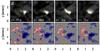
Fig. 4
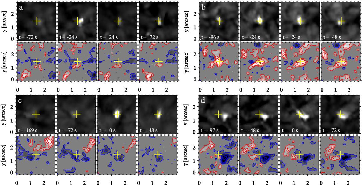
Four examples of magnetic field evolution around QSEBs. The four upper panels per sequence show Hα wing image cutouts at Δλ = −1 Å, the four lower panels corresponding Stokes V/Icont maps obtained from CRISP spectropolarimetry in Fe i 6173 Å. These are averages over 6 wing positions at Δλ = ± 0.150, ± 0.105, and ± 0.070 Å from line center. Signals below 3σnoise are put to 0 in the greyscaling, positive polarity is white with red contours, negative polarity is black with blue contours. The contour levels are at 0.2, 0.5, 1, and 2% polarization. The yellow cross at the center of each panel serves to guide inspection. a) and c) are from dataset 7 (μ = 0.73), b) and d) from dataset 8 (μ = 0.64). Animations of this figure are available in the on-line material. (Online movie.)
Current usage metrics show cumulative count of Article Views (full-text article views including HTML views, PDF and ePub downloads, according to the available data) and Abstracts Views on Vision4Press platform.
Data correspond to usage on the plateform after 2015. The current usage metrics is available 48-96 hours after online publication and is updated daily on week days.
Initial download of the metrics may take a while.