| Issue |
A&A
Volume 592, August 2016
|
|
|---|---|---|
| Article Number | A156 | |
| Number of page(s) | 8 | |
| Section | Stellar structure and evolution | |
| DOI | https://doi.org/10.1051/0004-6361/201628558 | |
| Published online | 24 August 2016 | |
The Solar Twin Planet Search
IV. The Sun as a typical rotator and evidence for a new rotational braking law for Sun-like stars⋆,⋆⋆
1 Universidade de São PauloDepartamento
de Astronomia do IAG/USP, Rua do Matão 1226, Cidade
Universitária, 05508-900 São
Paulo, SP, Brazil
e-mail: This email address is being protected from spambots. You need JavaScript enabled to view it.
2 University of Chicago,
Department of Astronomy and Astrophysics, IL
60637,
USA
3 Universidade Federal do Rio Grande do
Norte, 59072-970
Natal, RN, Brazil
4 Harvard-Smithsonian Center for
Astrophysics, Cambridge, MA
02138,
USA
5 University of Texas, McDonald Observatory and Department of
Astronomy at Austin, USA
6 The Australian National University,
Research School of Astronomy and Astrophysics, Cotter Road, Weston, ACT
2611,
Australia
7 University of Göttingen,
Institut für
Astrophysik, Germany
8 Universidade Federal do Rio Grande do
Sul, Instituto de Física, Av. Bento
Gonçalves 9500, 90650-002
Porto Alegre, RS, Brazil
Received:
19
March
2016
Accepted:
20
June
2016
Abstract
Context. It is still unclear how common the Sun is when compared to other similar stars in regards to some of its physical properties, such as rotation. Considering that gyrochronology relations are widely used today to estimate ages of stars in the main sequence, and that the Sun is used to calibrate it, it is crucial to assess whether these procedures are acceptable.
Aims. We analyze the rotational velocities, limited by the unknown rotation axis inclination angle, of an unprecedented large sample of solar twins to study the rotational evolution of Sun-like stars, and assess whether the Sun is a typical rotator.
Methods. We used high-resolution (R = 115 000) spectra obtained with the HARPS spectrograph and the 3.6 m telescope at La Silla Observatory. The projected rotational velocities for 81 solar twins were estimated by line profile fitting with synthetic spectra. Macroturbulence velocities were inferred from a prescription that accurately reflects their dependence with effective temperature and luminosity of the stars.
Results. Our sample of solar twins include some spectroscopic binaries with enhanced rotational velocities, and we do not find any nonspectroscopic binaries with unusually high rotation velocities. We verified that the Sun does not have a peculiar rotation, but the solar twins exhibit rotational velocities that depart from the Skumanich relation.
Conclusions. The Sun is a regular rotator when compared to solar twins with a similar age. Additionally, we obtain a rotational braking law that better describes the stars in our sample (v ∝ t-0.6) in contrast to previous, often-used scalings.
Key words: Sun: rotation / stars: solar-type / stars: rotation / stars: fundamental parameters
Based on observations collected at the European Organisation for Astronomical Research in the Southern Hemisphere under ESO programs 188.C-0265, 183.D-0729, 292.C-5004, 077.C-0364, 072.C-0488, 092.C-0721, 093.C-0409, 183.C-0972, 192.C-0852, 091.C-0936, 089.C-0732, 091.C-0034, 076.C-0155, 185.D-0056, 074.C-0364, 075.C-0332, 089.C-0415, 60.A-9036, 075.C-0202, 192.C-0224, 090.C-0421 and 088.C-0323.
Full Table 3 is only available at the CDS via anonymous ftp to cdsarc.u-strasbg.fr (130.79.128.5) or via http://cdsarc.u-strasbg.fr/viz-bin/qcat?J/A+A/592/A156
© ESO, 2016
1. Introduction
The Sun is the best-known star to astronomers and is commonly used as a template in the study of other similar objects. Yet, there are still some of its aspects that are not well understood and that are crucial for a better understanding of how stars and, consequently, how planetary systems and life evolve: how do the more complex physical parameters of a Sun-like star, such as rotation and magnetic activity, change with time? Is the Sun unique or typical (i.e., an average Sun-like star)? If the Sun is common, it would mean that life does not require a special star for it to flourish, eliminating the need to evoke an anthropic reasoning to explain it.
In an effort to assess how typical the Sun is, Robles et al. (2008) compared 11 of its physical parameters with nearby stars, and concluded that the Sun is, in general, typical. Although they found it to be a slow-rotator against 276 F8 – K2 (within ± 0.1M⊙) nearby stars, this result may be rendered inconclusive owing to unnacounted for noise that is caused by different masses and ages in their sample. Other studies have suggested that the Sun rotates either unusually slowly (Smith 1979; Leão et al. 2015) or regularly for its age (Soderblom 1983, 1985; Gray 1984; Gustafsson 1998; Barnes 2003), but none of these investigations comprised stars that are very similar to the Sun, therefore preventing a reliable comparison. In fact, with Kepler and CoRoT, it is now possible to obtain precise measurements of rotation periods, masses and ages of stars in a very homogeneous way (e.g., Ceillier et al. 2015; do Nascimento et al. 2012; Chaplin et al. 2014), but they generally lack high-precision stellar parameters, which are accessible through spectroscopy. The challenging nature of these observations limited ground-based efforts to smaller, but key stellar samples (e.g., Pizzolato et al. 2003; Strassmeier et al. 2012).
The rotational evolution of a star plays a crucial role in stellar interior physics and habitability. Previous studies proposed that rotation can produce extra mixing that is responsible for depleting the light elements Li and Be in their atmospheres (Pinsonneault et al. 1989; Charbonnel et al. 1994; Tucci Maia et al. 2015), which could explain the disconnection between meteoritic and solar abundances of Li (Baumann et al. 2010). Moreover, rotation is highly correlated with magnetic activity (e.g., Noyes et al. 1984; Soderblom et al. 1993; Baliunas et al. 1995; Mamajek & Hillenbrand 2008), and this trend is key to understanding how planetary systems and life evolve in face of varying magnetic activity and energy outputs by solar-like stars during the main sequence (Guinan & Engle 2009; Ribas et al. 2005; do Nascimento et al. 2016).
A theoretical treatment of rotational evolution from first principles is missing, so we often rely on empirical studies to make inferences about it. One of the pioneer efforts in this endeavor produced the well-known Skumanich relation v ∝ t− 1 / 2, where v is the rotational velocity and t is the stellar age (Skumanich 1972), which describes the rotational evolution of solar-type stars in the main sequence, and can be derived from the loss of angular momentum due to magnetized stellar winds (e.g., Kawaler 1988; Charbonneau 1992; Barnes 2003; Gallet & Bouvier 2013). This relation sparked the development of gyrochronology, which consists in estimating stellar ages based on their rotation, and it was shown to provide a stellar clock as good as chromospheric ages (Barnes 2007). In Skumanich-like relations, however, the Sun generally falls on the curve (or plane, if we consider dependence on mass) defined by the rotational braking law by design. Thus it is of utmost importance to assess how common the Sun is to correctly calibrate it.
Subsequent studies have proposed modifications to this paradigm of rotation and chromospheric activity evolution (e.g., Soderblom et al. 1991; Pace & Pasquini 2004), exploring rotational braking laws of the form v ∝ t− b. The formalism by Kawaler (1988) shows that this index b can be related to the geometry of the stellar magnetic field, and that the Skumanich index (b = 1 / 2) corresponds to a geometry that is slightly more complex than a simple radial field. It also dictates the dependence of the angular momentum on the rotation rate and, in practice, it determines how early the effects of braking are felt by a model. Such prescriptions for rotational evolution have a general agreement for young ages up to the solar age (see Sood et al. 2016; Amard et al. 2016, and references therein), but the evolution for older ages still poses an open question. In particular, van Saders et al. (2016) suggested that stars undergo a weakened magnetic braking after they reach a critical value of the Rossby number, thus explaining the stagnation trend observed on the rotational periods of older Kepler stars.
In order to assess how typical the Sun is in its rotation, our study aims to verify whether the Sun follows the rotational evolution of stars that are very similar to it, which is an objective that is achieved by precisely measuring their rotational velocities and ages. We take advantage of an unprecedented large sample of solar twins (Ramírez et al. 2014) using high signal to noise (S/N> 500) and high-resolution (R> 105) spectra, which provides us with precise stellar parameters and is essential for the analysis that we perform (see Fig. 1 for an illustration of the subtle effects of rotation in stellar spectra of Sun-like stars).
2. Working sample
Our sample consists of bright solar twins in the Southern Hemisphere, which were mostly observed in our HARPS Large Program (ID: 188.C-0265) at the European Southern Observatory (ESO) that aimed to search for planetary systems around stars very similar to the Sun (Ramírez et al. 2014; Bedell et al. 2015; Tucci Maia et al. 2016, Papers I, II and III, respectively, of the series The Solar Twin Planet Search). These stars are loosely defined as those that have Teff, log g and [Fe/H] inside the intervals ± 100 K, ± 0.1 [cgs] and 0.1 dex, respectively, around the solar values. It has been shown that these limits guarantee ~0.01 dex precision in the relative abundances derived using standard model atmosphere methods and that the systematic uncertainties of that analysis are negligible within those ranges (Bedell et al. 2014; Biazzo et al. 2015; Saffe et al. 2015; Yana Galarza et al. 2016). In total, we obtained high-precision spectra for 73 stars and used data from 9 more targets observed in other programs; all of these overlapped the sample of 88 stars from Paper I. We used the spectrum of the Sun (reflected light from the Vesta asteroid) from the ESO program 088.C-0323, which was obtained with the same instrument and configuration as the solar twins.
The ages of the solar twin sample span between 0−10 Gyr and are presented in Table 3. They were obtained by Tucci Maia et al. (2016) using Yonsei-Yale isochrones (Yi et al. 2001) and probability distribution functions as described in Ramírez et al. (2013, 2014). Uncertainties are assumed to be symmetric. These ages are in excellent agreement with those obtained in Paper I, with a mean difference of −0.1 ± 0.2 Gyr (see footnote 5 in Paper III). We adopted 4.56 Gyr for the solar age (Bahcall et al. 1995). The other stellar parameters (Teff, log g, [Fe/H] and microturbulence velocities vt) were obtained by Ramírez et al. (2014). The stellar parameters of HIP 68468 and HIP 108158 were updated by Tucci Maia et al. (2016).
Our targets were observed at the HARPS spectrograph (Mayor et al. 2003), which is fed by ESO’s 3.6 m telescope at La Silla Observatory. When available publicly, we also included all observations from other programs in our analysis in order to increase the signal-to-noise ratio (S/N) of our spectra. However, we did not use observations for 18 Sco (HIP 79672) from May 2009, owing to their instrumental artifacts, and we did not include observations post-HARPS upgrade (June 2015) when combining the spectra – they had a different shape in the red side, and since there were few observations, we chose not to use them to eliminate eventual problems with combination and normalization. Our initial plan was to use the observations from the MIKE spectrograph, as described by the Paper I. However, we decided to use the HARPS spectra due to its higher spectral resolving power.
The wavelength coverage for the observations ranged from 3780 to 6910 Å, with a spectral resolving power of R = λ/ Δλ = 115 000. Data reduction was performed automatically with the HARPS Data Reduction Software (DRS). Each spectrum was divided into two halves, corresponding to the mosaic of two detectors (one optimized for blue and other for red wavelengths). In this study we only worked with the red part (from 5330 to 6910 Å) because of its higher S/N and the presence of cleaner lines. The correction for radial velocities was performed with the task dopcor from IRAF1, using the values obtained from the cross-correlation function (CCF) of the pipeline. The different observations were combined with IRAF’s scombine. The resulting average (of the sample) signal to noise ratio was 500 around 6070 Å. The red regions of the spectra were normalized with ~30th order polynomial fits to the upper envelopes of the entire red range, using the task continuum on IRAF. We made sure that the continuum of the stars were consistent with the Sun’s. Additionally, we verified that errors in the continuum determination introduce uncertainties in vsini lower than 0.1 km s-1.
 |
Fig. 1 Comparison of the spectral line broadening between two solar twins with different projected rotational velocities. The wider line corresponds to HIP 19911, with vsini ≈ 4.1 km s-1, and the narrower line comes from HIP 8507, with vsini ≈ 0.8 km s-1. |
3. Methods
We analyzed five spectral lines, four due to Fe I and one to Ni I (see Table 1; equivalent widths were measured using the task splot in IRAF), which were selected for having low levels of contamination by blending lines. The rotational velocity of a star can be measured by estimating the spectral line broadening that is due to rotation. The rotation axes of the stars are randomly oriented, thus the spectroscopic measurements of rotational velocity are a function of the inclination angle (vsini).
Line list used in the projected stellar rotation measurements.
We estimate vsini for our sample of solar twins using the 2014 version of MOOG Synth (Sneden 1973), adopting stellar atmosphere models by Castelli & Kurucz (2004), with interpolations between models performed automatically by the Python package qoyllur-quipu2 (see Ramírez et al. 2014). The instrumental broadening is taken into account by the spectral synthesis. We used the stellar parameters from Tucci Maia et al. (2016) and microturbulence velocities from Ramírez et al. (2014). Macroturbulence velocities (vmacro) were calculated by scaling the solar values, line by line (see Sect. 3.1). An estimation of the rotational velocities was performed with our own algorithm3 that makes automatic measurements for all spectral lines for each star. We applied fine-tuning corrections by eye for the nonsatisfactory automatic line profile fittings, and quote vsini as the mean of the values measured for the five lines. See Sects. 3.1 and 3.2 for a detailed description on rotational velocities estimation and their uncertainties. Figure 2 shows an example of spectral line fitting for one feature in the Sun.
 |
Fig. 2 Example of line profile fitting for the Fe I feature at 6151.62 Å in the spectrum of the Sun. The continuous curve is the synthetic spectrum, and the open circles are the observed data. |
3.1. Macroturbulence velocities
We tested the possibility of measuring vmacro (radial-tangential profile) simultaneously with vsini, but even when using the extremely high-resolution spectra of HARPS, it is difficult to disentangle these two spectral line broadening processes; this is probably because of the low values of these velocities. Macroturbulence has a stronger effect on the wings of the spectral lines, but our selection of clean lines still has some contamination that requires this high-precision work to be carried out by eye. Some stars show more contamination than others, complicating the disentaglement. Fortunately, the variation of macroturbulence with effective temperature and luminosity is smooth (Gray 2005), so that precise values of vmacro could be obtained by a calibration. Thus we adopted a relation that fixes macroturbulence velocities to measure vsini with high precision using an automatic code, which provides the additional benefits of reproducibility and lower subjectivity.
The macroturbulence velocity is known to vary for different spectral lines (Gray 2005), so for our high-precision analysis we do not adopt a single value for each star. Instead, we measure the vmacro for the Sun in each of the spectral lines from Table 1 and use these values to scale the vmacro for all stars in our sample using the following equation4: 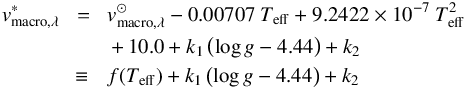 (1)where
  is the macroturbulence velocity of the Sun for a given spectral line, Teff and log g are the effective temperature and gravity of a given star, respectively, k1 is a proportionality factor for log g and k2 is a small correction constant.
This formula is partly based on the relation derived by Meléndez et al. (2012; Eq. (E.1) in their paper) from the trend of macroturbulence with effective temperature in solar-type stars described by Gray (2005). The log g-dependent term (a proxy for luminosity) comes from the empirical relation derived by Doyle et al. (2014; Eq. (8) in their paper), and is based on spectroscopic measurements of vmacro of Kepler stars, which were disentangled from vsini using asteroseismic estimates of the projected rotational velocities. Doyle et al. obtained a value for the proportionality factor k1 of −2.0. Their uncertainties on vmacro, however, were on the order of 1.0 km s-1. Thus, we decided to derive our own values of k1 and k2 by simultaneously measuring vmacro and vsini of a subsample of solar twins.
This subsample was chosen to contain only single stars or visual binaries mostly in the extremes of log g (4.25−4.52) in our entire sample. We assume these values have a linear relationship with vmacro inside this short interval of log g. We used as a first guess the values of vsini and vmacro from a previous, cruder estimation we made, and performed line profile fits by eye using MOOG Synth. The velocities in Table 2 are the median of the values measured for each line and their standard error. These vsini are not consistently measured in the same way as the final results. The rotational velocity broadening was calculated by our own code (see Sect. 3.2 for details). By performing a linear fit in the vmacro − f(Teff) versus log g − 4.44 relation (f comprises all the Teff-dependent terms, the macroturbulence velocity of the Sun and the known constant on Eq. (1)), we obtain that k1 = −1.81 ± 0.26 and k2 = −0.05 ± 0.03 (see Fig. 3). For the stars farthest from the Sun in log g from our sample, these values of k1 and k2 would amount to differences of up to ± 0.4 km s-1 in their macroturbulence velocities, therefore it is essential to consider the luminosity effect on vmacro for accurate vsini determinations.
Simultaneous measurements of rotational and macroturbulence velocities of stars in the extremes of log g from our sample of solar twins.
 |
Fig. 3 Linear relation between vmacro and log g (a proxy for luminosity) for the stars on Table 2. See the definition of f(Teff) in Sect. 3.1. The orange continuous line represents our determination of a proportionality coefficient of −1.81 and a vertical shift of −0.05 km s-1. The black dashed line is the coefficient found by Doyle et al. (2014). The light gray region is a composition of 200 curves with parameters drawn from a multivariate Gaussian distribution. The Sun is located at the origin. |
To obtain the macroturbulence velocities for the Sun to use in Eq. (1), we forced the rotational velocity of the Sun to 1.9 km s-1 (Howard & Harvey 1970), and then estimated values of  by fitting each line profile using MOOG Synth, and the results are shown in Table 1. We estimated the error in determining to be ± 0.1 km s-1. Since Eq. (1) is an additive scaling, the error for vmacro of all stars is the same as in the Sun. The uncertainties in stellar parameters have contributions that are negligible compared to the ones introduced by the error in vmacro.
3.2. Rotational velocities
Our code takes as input the list of stars and their parameters (effective temperature, surface gravity, metallicity and microturbulence velocities obtained on Paper I), their spectra and the spectral line list in MOOG-readable format. For each line in a given star, the code automatically corrects the spectral line shift and the continuum. The first is performed by fitting a second-order polynomial to the kernel of a line and estimating the distance of the observed line center from the laboratory value. Usually, the spectral line shift corrections were on the order of 10-2 Å, corresponding to 0.5 km s-1 in the wavelength range we worked on. This is a reasonable shift that likely arises from a combination of granulation and gravitational redshift effects, which are of similar magnitude. The continuum correction for each line is defined as the value of a multiplicative factor that sets the highest flux inside a radius of 2.5 Å around the line center to 1.0. The multiplicative factor usually has a value inside the range 1.000 ± 0.002.
Ages, the measured vsini, and stellar parameters of the solar twins and the Sun.
The code starts with a range of vsini and abundances and optimizes these two parameters through a series of iterations that measure the least-squares difference between the observed line and the synthetic line (generated with MOOG synth). Convergence is achieved when the difference between the best and previous solutions, for both vsini and abundance, is less than 1%. Additionally, the code also forces at least ten iterations to avoid falling into local minima.
One of the main limitations of MOOG Synth for our analysis is that it has a “quantized” behavior for vsini: the changes in the synthetic spectra occur most strongly in steps of 0.5 km s-1. This behavior is not observed in varying the macroturbulence velocities. Therefore, we had to incorporate a rotational broadening routine in our code that was separated from MOOG. We used the Eq. (18.14) from Gray (2005), in velocity space, to compute the rotational profile5![Mathematical equation: \begin{equation} G(v) = \frac{2(1-\epsilon)\left[ 1-(v/v\rm_L)^2 \right]^{1/2} + \frac{1}{2} \pi \epsilon \left[ 1-(v/v\rm_L)^2 \right]}{\pi v\rm_L (1-\epsilon/3)}, \end{equation}](/articles/aa/full_html/2016/08/aa28558-16/aa28558-16-eq75.png) (2)where vL is the projected rotational velocity and ϵ is the limb darkening coefficient (for which we adopt the value 0.6). The rotational profile G(v) is then convolved with the MOOG synthetic profiles, which were generated with vsini = 0.
(2)where vL is the projected rotational velocity and ϵ is the limb darkening coefficient (for which we adopt the value 0.6). The rotational profile G(v) is then convolved with the MOOG synthetic profiles, which were generated with vsini = 0.
The total uncertainties in rotational velocities are obtained from the quadratic sum of the standard error of the five measurements and an uncertainty of 0.1 km s-1 introduced by the error in macroturbulence velocities. Systematic errors in the calculation of vmacro,λ for the stars do not significantly contribute to the vsini uncertainties. The rotational velocities we measured and their uncertainties are reproduced in Table 3.
Some of the stars in the sample show very low rotational velocities, most probably owing to the effect of projection (see left panel of Fig. 5). The achieved precision is validated by comparison with the values of the full width at half maximum (FWHM) measured by the cross-correlation function (CCF) from the data reduction pipeline, with the effects of macroturbulence subtracted (see Fig. 4). The spectroscopic binary star HIP 103983 has an unusually high vsini when compared to the CCF FWHM, and a verification of its spectral line profiles reveals the presence of distortions, which are the most probably caused by mismeasurement of rotational velocity (contamination of the combined spectrum by a companion; observations range from October 2011 to August 2012). We obtained a curve fit for the vsini versus CFF FWHM (km s-1) using a similar relation as used by Melo et al. (2001), Pace & Pasquini (2004), Hekker & Meléndez (2007), which resulted in the following calibration: vsini=![Mathematical equation: \hbox{$\sqrt{(0.73 \pm 0.02) \left[\textit{FWHM}^2 - v_{\mathrm{macro}}^2 - (5.97 \pm 0.01)^2\right]}$}](/articles/aa/full_html/2016/08/aa28558-16/aa28558-16-eq81.png) km s-1 (estimation performed with the MCMC code emcee6Foreman-Mackey et al. 2013). The scatter between the measured vsini and those estimated from CCF is σ = 0.20 km s-1 (excluding the outlier HIP 103983). The typical uncertainty in the rotational velocities we obtain with our method, that is, line profile fitting with extreme high-resolution spectra, is 0.12 km s-1, which implies that the average error of the CCF FWHM vsini scaling is 0.16 km s-1. This average error could be significantly higher if the broadening by vmacro is not accounted for.
km s-1 (estimation performed with the MCMC code emcee6Foreman-Mackey et al. 2013). The scatter between the measured vsini and those estimated from CCF is σ = 0.20 km s-1 (excluding the outlier HIP 103983). The typical uncertainty in the rotational velocities we obtain with our method, that is, line profile fitting with extreme high-resolution spectra, is 0.12 km s-1, which implies that the average error of the CCF FWHM vsini scaling is 0.16 km s-1. This average error could be significantly higher if the broadening by vmacro is not accounted for.
 |
Fig. 4 Comparison between our estimated values of vsini (y-axis) and those inferred from the cross-correlation funcion FWHM (x-axis). The spread around the 1:1 relation (black line) is σ = 0.20 km s-1. |
 |
Fig. 5 Projected rotational velocity of solar twins as a function of their age. The Sun is represented by the symbol ⊙. Left panel: all stars of our sample; the orange triangles are spectroscopic binaries, blue circles are the selected sample and the blue dots are the remaining nonspectroscopic binaries. Right panel: the rotational braking law; the purple continuous curve is our relation inferred from fitting the selected sample (blue circles) of solar twins with the form vsini = vf + mt− b, where t is the stellar age, and the fit parameters are vf = 1.224 ± 0.447, m = 1.932 ± 0.431, and b = 0.622 ± 0.354, with vf and b highly and positively correlated. The light gray region is composed of 300 curves that are created with parameters drawn from a multivariate Gaussian distribution defined by the mean values of the fit parameters and their covariance matrix. Skumanich’s law (red × symbols, calibrated for |

4. Binary stars
We identified 16 spectroscopic binaries (SB) in our sample of 81 solar twins by analyzing their radial velocities; some of these stars are reported as binaries by Tokovinin (2014a,b), Mason et al. (2001), Baron et al. (2015). We did not find previous reports of multiplicity for the stars HIP 30037, HIP 62039 and HIP 64673 in the literature. Our analysis of variation in the HARPS radial velocities suggest that the first two are probable SBs, while the latter is a candidate. No binary shows a double-lined spectrum, but HIP 103983 has distortions that could be from contamination by a companion. The star HIP 64150 is a Sirius-like system with a directly observed white dwarf companion (Crepp et al. 2013; Matthews et al. 2014). The sample from Paper I contains another SB, HIP 109110, for which we could not reliably determine the vsini because of strong contamination in the spectra, which is possibly caused by a relatively bright companion. Thus, we did not include this star in our sample.
Of these 16 spectroscopic binaries, at least four of them (HIP 19911, 43297, 67620 and 73241) show unusually high vsini (see the left panel of Fig. 5). These stars also present other anormalities, such as their [Y/Mg] abundances (Tucci Maia et al. 2016) and magnetic activity (Ramírez et al. 2014; Freitas et al., in prep.). The solar twin blue straggler HIP 10725 (Schirbel et al. 2015), which is not included in our sample, also shows a high vsini for its age. We find that five of the binaries have rotational velocities below the expected for Sun-like stars, but this is most likely an effect of projection of the rotational axes of the stars. For the remaining binaries, which follow the rotational braking law, it is again difficult to disentangle this behavior from the sini, and a statistical analysis is precluded by the low numbers involved. Tidal interactions between companions that could potentially enhance rotation depend on binary separation, which is unknown for most of these stars. They should be regular rotators, since they do not show anormalities in chromospheric activity (Freitas et al., in prep.) or [Y/Mg] abundances (Tucci Maia et al. 2016).
Based on the information that at least 25% of the spectroscopic binaries in our sample show higher rotational velocities than expected for single stars, we conclude that stellar multiplicity is an important enhancer of rotation in Sun-like stars. Blue stragglers are expected to have a strong enhancement on rotation owing to injection of angular momentum from the donor companion.
5. The rotational braking law
We removed from this analysis all the spectroscopic binaries in order to correctly constrain the rotational braking. The non-SB HIP 29525 displays a vsini that is much higher than expected (3.85 ± 0.13 km s-1), but it is likely that this is the result of an overestimated isochronal age (2.83 ± 1.06 Gyr). We decided to not include HIP 29525 in the rotational braking determination because it is a clear outlier in our results. Maldonado et al. (2010) found X-ray and chromospheric ages of 0.55 and 0.17 Gyr, respectively, for HIP 29525. We then divided the remaining 65 stars and the Sun in bins of 2 Gyr, and removed all the stars that were below the 70th percentile of vsini in each bin from this sample. Such a procedure can be justified because we verified that 30% of the stars should have sini above 0.9 by doing a simple simulation with angles i drawn from a flat distribution between 0 and π/ 2. This allowed us to select the stars that had the highest chance of having sini above 0.9. In total, 21 solar twins and the Sun compose what we hereafter reference as the selected sample. Albeit this subsample is smaller, it has the advantage of mostly removing uncertainties on the inclination angle of the stellar rotation axes7. We stress that the only reason we can select the most probable edge-on rotating stars (i = π/ 2) is because we have a large sample of solar twins in the first place.
We then proceeded to fit a general curve to the selected sample (see Fig. 5) using the method of orthogonal distance regression (ODR, Boggs & Rogers 1990), which takes the uncertainties on both vsini and ages into account. This curve is a power law plus constant of the form v = vf + mt− b (the same chromospheric activity and vsini vs. age relation used by Pace & Pasquini 2004; Guinan & Engle 2009), with v (rotational velocity) and vf (asymptotic velocity) in km s-1 and t (age) in Gyr.
We find that the best-fit parameters are vf = 1.224 ± 0.447, m = 1.932 ± 0.431, and b = 0.622 ± 0.354 (see right panel of Fig. 5). These large uncertainties are likely due to i) the strong correlation between vf and b; and ii) the relatively limited number of data points between 1 and 4 Gyr, where the parameters are most effective in changing the values of v. This limitation is also present in past studies (e.g., van Saders et al. 2016; Barnes 2003; Pace & Pasquini 2004; Mamajek & Hillenbrand 2008; García et al. 2014; Amard et al. 2016). On the other hand, our sample is the largest comprising solar twins and, therefore, should produce more reliable results. With more data points, we could be able to use 1 Gyr bins instead of 2 Gyr in order to select the fastest rotating stars, which would result in a better subsample for constraining the rotational evolution for young stars.
The relation we obtain is in contrast with some previous studies on modeling the rotational braking (Barnes 2001, 2003; Lanzafame & Spada 2015) which either found or assumed that the Skumanich law explains well the rotational braking of Sun-like stars. The conclusions by van Saders et al. (2016) limit the range of validation up to approximately the solar age (4 Gyr) for stars with solar mass. When we enforce the Skumanich power-law index b = 1 / 2, we obtain a worse fit between the ages 2 and 4 Gyr and, not surprisingly, after the solar age as well.
Our data and the rotational braking law that results from them show that the Sun is a normal star regarding its rotational velocity when compared to solar twins. However, they do not agree with the regular Skumanich law (Barnes 2007, red × symbols in Fig. 5). We find a better agreement with the model proposed by do Nascimento et al. (2014, black dashed curve in Fig. 5, especially for stars older than 2 Gyr. This model is thoroughly described in Appendix A of do Nascimento et al. (2012). In summary, this model uses an updated treatment of the instabilities that are relevant to the transport of angular momentum, according to Zahn (1992) and Talon & Zahn (1997), with an initial angular momentum for the Sun J0 = 1.63 × 1050 g cm2 s-1. The rotational braking curve that corresponds to the model by do Nascimento et al. (2014) is computed using the output radii of the model, which vary from ~1 R⊙ at the current solar age to 1.57 R⊙ at the age of 11 Gyr, and it changes significantly if we use a constant radius R = 1 R⊙. This results in a more Skumanich-like rotational braking.
Our result agrees with the chromospheric activity versus age behavior for solar twins obtained by Ramírez et al. (2014), in which a steep decay of the  index during the first 4 Gyr was deduced (see Fig. 11 in their paper). The study by Pace & Pasquini (2004) also suggests a steeper power-law index (b = 1.47) than Skumanich’s (bS = 1 / 2) in the rotational braking law derived from young open clusters, the Sun and M 67. As seen in Fig. 5, however, their relation significantly overestimates the rotational velocities of stars, especially for those older than 2 Gyr. This is most probably caused by other line broadening processes, mainly the macroturbulence, which were not considered in that study. As we saw in Sect. 3.1, those processes introduce important effects that are sometimes larger than the rotational broadening. Moreover, a CCF-only analysis tends to produce more spread in the vsini than the more detailed analysis we used.
The rotational braking law we obtain produces a similar outcome to that achieved by van Saders et al. (2016) for stars older than the Sun, that is, a weaker rotational braking law after solar age than previously suggested. Our data also requires a different power-law index than the Skumanich index for stars younger than the Sun, accounting for an earlier decay of rotational velocities up to 2 Gyr.
The main-sequence spin-down model by Kawaler (1988) states that, for constant moment of inertia and radius during the main sequence, we would have  (3)where veq is the rotational velocity at the equator and a and n are parameters that measure the dependence on rotation rate and radius, respectively (see Eqs. (7), (8) and (12) in their paper). If we assume a dipole geometry for the stellar magnetic field (Br ∝ B0r3), then n = 3 / 7. Furthermore, assuming that a = 1, then Eq. (3) results in veq ∝ t− 7 / 4 = t-1.75. The Skumanich law (veq ∝ t-0.5) is recovered for n = 3 / 2, which is close to the case of a purely radial field (n = 2, veq ∝ t-0.38). A more extensive exploration of the configuration and evolution of magnetic fields of solar twins is outside the scope of this paper, but our results suggest that the rotational rotational braking we observe on this sample of solar twins stems from a magnetic field with an intermediate geometry between dipole and purely radial.
6. Conclusions
We analyzed the rotational velocities of 81 bright solar twins in the Southern Hemisphere and the Sun using extremely high-resolution spectra. Radial velocities revealed that our sample contained 16 spectroscopic binaries, 3 of which (HIP 30037, 62039, 64673) were not listed as such in the literature. At least 5 of these stars show an enhancement on their measured vsini, which is probably caused by interaction with their close-by companions. They also present other anomalies in chemical abundances and chromospheric activities. We did not clearly identify nonspectroscopic binary stars with unusually high rotational velocities for their age.
We selected a subsample of stars with higher chances of having their rotational axis inclination close to π/ 2 (almost edge-on) in order to better constrain the rotational evolution of the solar twins. We opted to use carefully measured isochronal ages for these stars because it is the most reliable method available for this sample. We finally conclude that the Sun seems to be a common rotator, within our uncertainties, when compared to solar twins, therefore it can be used to calibrate stellar models.
Moreover, we have found that the Skumanich law does not describe well the rotation evolution for solar twins observed in our data, which is a discrepancy that is stronger after the solar age. Therefore, we propose a new rotational braking law that supports the weakened braking after the age of the Sun, and comes with a earlier decay in rotational velocities up to 2 Gyr than the classical Skumanich’s law. Interestingly, it also reveals an evolution that is more similar to the magnetic activity evolution observed in Sun-like stars, which sees a steep decay in the first 3 Gyr and flattens near the solar age. Additionally, we suggest that more high-precision spectroscopic observations of solar twins younger and much older than the Sun could help us better constrain the rotational evolution of solar-like stars.
IRAF is distributed by the National Optical Astronomy Observatories, which are operated by the Association of Universities for Research in Astronomy, Inc., under cooperative agreement with the National Science Foundation.
Available at https://github.com/astroChasqui/q2
Available at https://github.com/RogueAstro/PoWeRS
In the future, it should be possible to calibrate macroturbulence velocities using 3D hydrodynamical stellar atmosphere models (e.g., Magic et al. 2013) by using predicted 3D line profiles (without rotational broadening) as observations and determine which value of vmacro is needed to reproduce them with 1D model atmospheres.
This is the same recipe adopted by the radiative transfer code MOOG.
Available at http://dan.iel.fm/emcee/current/
This procedure can also allow for unusually fast-rotating stars (although rare) with sini below 0.9 to leak into the subsample.
Acknowledgments
L.d.S. thanks CAPES and FAPESP, grants No. 2014/26908-1 and 2016/01684-9 for support. J.M. thanks FAPESP (2012/24392-2) for support. L.S. acknowledges support by FAPESP (2014/15706-9). We also would like to thank the anonymous referee for valuable comments that significantly improved this manuscript.
References
- Amard, L., Palacios, A., Charbonnel, C., Gallet, F., & Bouvier, J. 2016, A&A, 587, A105 [NASA ADS] [CrossRef] [EDP Sciences] [Google Scholar]
- Bahcall, J. N., Pinsonneault, M. H., & Wasserburg, G. J. 1995, Rev. Mod. Phys., 67, 781 [NASA ADS] [CrossRef] [Google Scholar]
- Baliunas, S. L., Donahue, R. A., Soon, W. H., et al. 1995, ApJ, 438, 269 [NASA ADS] [CrossRef] [Google Scholar]
- Barnes, S. A. 2001, ApJ, 561, 1095 [NASA ADS] [CrossRef] [Google Scholar]
- Barnes, S. A. 2003, ApJ, 586, 464 [NASA ADS] [CrossRef] [Google Scholar]
- Barnes, S. A. 2007, ApJ, 669, 1167 [NASA ADS] [CrossRef] [Google Scholar]
- Baron, F., Lafrenière, D., Artigau, É., et al. 2015, ApJ, 802, 37 [NASA ADS] [CrossRef] [Google Scholar]
- Baumann, P., Ramírez, I., Meléndez, J., Asplund, M., & Lind, K. 2010, A&A, 519, A87 [NASA ADS] [CrossRef] [EDP Sciences] [Google Scholar]
- Bedell, M., Meléndez, J., Bean, J. L., et al. 2014, ApJ, 795, 23 [NASA ADS] [CrossRef] [Google Scholar]
- Bedell, M., Meléndez, J., Bean, J. L., et al. 2015, A&A, 581, A34 [NASA ADS] [CrossRef] [EDP Sciences] [Google Scholar]
- Biazzo, K., Gratton, R., Desidera, S., et al. 2015, A&A, 583, A135 [NASA ADS] [CrossRef] [EDP Sciences] [Google Scholar]
- Boggs, P. T., & Rogers, J. E. 1990, Contemporary Mathematics, 112, 183 [Google Scholar]
- Castelli, F., & Kurucz, R. L. 2004, ArXiv e-prints [arXiv:astro-ph/0405087] [Google Scholar]
- Ceillier, T., García, R. A., Salabert, D., & Mathur, S. 2015, in EPJ Web Conf., 101, 06016 [Google Scholar]
- Chaplin, W. J., Basu, S., Huber, D., et al. 2014, ApJS, 210, 1 [NASA ADS] [CrossRef] [Google Scholar]
- Charbonneau, P. 1992, in Cool Stars, Stellar Systems, and the Sun, eds. M. S. Giampapa, & J. A. Bookbinder, ASP Conf. Ser., 26, 416 [Google Scholar]
- Charbonnel, C., Vauclair, S., Maeder, A., Meynet, G., & Schaller, G. 1994, A&A, 283, 155 [NASA ADS] [Google Scholar]
- Crepp, J. R., Johnson, J. A., Howard, A. W., et al. 2013, ApJ, 774, 1 [NASA ADS] [CrossRef] [Google Scholar]
- do Nascimento, J.-D., da Costa, J. S., & Castro, M. 2012, A&A, 548, L1 [NASA ADS] [CrossRef] [EDP Sciences] [Google Scholar]
- do Nascimento, Jr., J.-D., García, R. A., Mathur, S., et al. 2014, ApJ, 790, L23 [NASA ADS] [CrossRef] [Google Scholar]
- do Nascimento, Jr., J.-D., Vidotto, A. A., Petit, P., et al. 2016, ApJ, 820, L15 [NASA ADS] [CrossRef] [Google Scholar]
- Doyle, A. P., Davies, G. R., Smalley, B., Chaplin, W. J., & Elsworth, Y. 2014, MNRAS, 444, 3592 [NASA ADS] [CrossRef] [Google Scholar]
- Foreman-Mackey, D., Hogg, D. W., Lang, D., & Goodman, J. 2013, PASP, 125, 306 [CrossRef] [Google Scholar]
- Gallet, F., & Bouvier, J. 2013, A&A, 556, A36 [NASA ADS] [CrossRef] [EDP Sciences] [Google Scholar]
- García, R. A., Ceillier, T., Salabert, D., et al. 2014, A&A, 572, A34 [NASA ADS] [CrossRef] [EDP Sciences] [Google Scholar]
- Gray, D. F. 1984, ApJ, 281, 719 [NASA ADS] [CrossRef] [Google Scholar]
- Gray, D. F. 2005, The Observation and Analysis of Stellar Photospheres (CUP) [Google Scholar]
- Guinan, E. F., & Engle, S. G. 2009, in The Ages of Stars, eds. E. E. Mamajek, D. R. Soderblom, & R. F. G. Wyse, IAU Symp., 258, 395 [Google Scholar]
- Gustafsson, B. 1998, Space Sci. Rev., 85, 419 [NASA ADS] [CrossRef] [Google Scholar]
- Hekker, S., & Meléndez, J. 2007, A&A, 475, 1003 [NASA ADS] [CrossRef] [EDP Sciences] [Google Scholar]
- Howard, R., & Harvey, J. 1970, Sol. Phys., 12, 23 [NASA ADS] [CrossRef] [Google Scholar]
- Kawaler, S. D. 1988, ApJ, 333, 236 [NASA ADS] [CrossRef] [Google Scholar]
- Lanzafame, A. C., & Spada, F. 2015, A&A, 584, A30 [NASA ADS] [CrossRef] [EDP Sciences] [Google Scholar]
- Leão, I. C., Pasquini, L., Ferreira Lopes, C. E., et al. 2015, A&A, 582, A85 [NASA ADS] [CrossRef] [EDP Sciences] [Google Scholar]
- Magic, Z., Collet, R., Asplund, M., et al. 2013, A&A, 557, A26 [NASA ADS] [CrossRef] [EDP Sciences] [Google Scholar]
- Maldonado, J., Martínez-Arnáiz, R. M., Eiroa, C., Montes, D., & Montesinos, B. 2010, A&A, 521, A12 [NASA ADS] [CrossRef] [EDP Sciences] [Google Scholar]
- Mamajek, E. E., & Hillenbrand, L. A. 2008, ApJ, 687, 1264 [NASA ADS] [CrossRef] [Google Scholar]
- Mason, B. D., Hartkopf, W. I., Holdenried, E. R., & Rafferty, T. J. 2001, AJ, 121, 3224 [NASA ADS] [CrossRef] [Google Scholar]
- Matthews, C. T., Crepp, J. R., Skemer, A., et al. 2014, ApJ, 783, L25 [NASA ADS] [CrossRef] [Google Scholar]
- Mayor, M., Pepe, F., Queloz, D., et al. 2003, The Messenger, 114, 20 [NASA ADS] [Google Scholar]
- Meléndez, J., Bergemann, M., Cohen, J. G., et al. 2012, A&A, 543, A29 [NASA ADS] [CrossRef] [EDP Sciences] [Google Scholar]
- Melo, C. H. F., Pasquini, L., & De Medeiros, J. R. 2001, A&A, 375, 851 [NASA ADS] [CrossRef] [EDP Sciences] [Google Scholar]
- Noyes, R. W., Hartmann, L. W., Baliunas, S. L., Duncan, D. K., & Vaughan, A. H. 1984, ApJ, 279, 763 [NASA ADS] [CrossRef] [Google Scholar]
- Pace, G., & Pasquini, L. 2004, A&A, 426, 1021 [NASA ADS] [CrossRef] [EDP Sciences] [Google Scholar]
- Pinsonneault, M. H., Kawaler, S. D., Sofia, S., & Demarque, P. 1989, ApJ, 338, 424 [NASA ADS] [CrossRef] [Google Scholar]
- Pizzolato, N., Maggio, A., Micela, G., Sciortino, S., & Ventura, P. 2003, A&A, 397, 147 [NASA ADS] [CrossRef] [EDP Sciences] [Google Scholar]
- Ramírez, I., Allen de Prieto, C., & Lambert, D. L. 2013, ApJ, 764, 78 [NASA ADS] [CrossRef] [Google Scholar]
- Ramírez, I., Meléndez, J., Bean, J., et al. 2014, A&A, 572, A48 [NASA ADS] [CrossRef] [EDP Sciences] [Google Scholar]
- Ribas, I., Guinan, E. F., Güdel, M., & Audard, M. 2005, ApJ, 622, 680 [NASA ADS] [CrossRef] [Google Scholar]
- Robles, J. A., Lineweaver, C. H., Grether, D., et al. 2008, ApJ, 684, 691 [NASA ADS] [CrossRef] [Google Scholar]
- Saffe, C., Flores, M., & Buccino, A. 2015, A&A, 582, A17 [NASA ADS] [CrossRef] [EDP Sciences] [Google Scholar]
- Schirbel, L., Meléndez, J., Karakas, A. I., et al. 2015, A&A, 584, A116 [NASA ADS] [CrossRef] [EDP Sciences] [Google Scholar]
- Skumanich, A. 1972, ApJ, 171, 565 [NASA ADS] [CrossRef] [Google Scholar]
- Smith, M. A. 1979, PASP, 91, 737 [NASA ADS] [CrossRef] [Google Scholar]
- Sneden, C. A. 1973, Ph.D. Thesis, The University of Texas at Austin [Google Scholar]
- Soderblom, D. R. 1983, ApJS, 53, 1 [NASA ADS] [CrossRef] [Google Scholar]
- Soderblom, D. R. 1985, AJ, 90, 2103 [NASA ADS] [CrossRef] [Google Scholar]
- Soderblom, D. R., Duncan, D. K., & Johnson, D. R. H. 1991, ApJ, 375, 722 [NASA ADS] [CrossRef] [Google Scholar]
- Soderblom, D. R., Stauffer, J. R., Hudon, J. D., & Jones, B. F. 1993, ApJS, 85, 315 [NASA ADS] [CrossRef] [Google Scholar]
- Sood, A., Kim, E.-j., & Hollerbach, R. 2016, ApJ, submitted [arXiv:1605.07125] [Google Scholar]
- Strassmeier, K. G., Weber, M., Granzer, T., & Järvinen, S. 2012, Astron. Nachr., 333, 663 [NASA ADS] [CrossRef] [Google Scholar]
- Talon, S., & Zahn, J.-P. 1997, A&A, 317, 749 [Google Scholar]
- Tokovinin, A. 2014a, AJ, 147, 86 [NASA ADS] [CrossRef] [Google Scholar]
- Tokovinin, A. 2014b, AJ, 147, 87 [NASA ADS] [CrossRef] [Google Scholar]
- Tucci Maia, M., Meléndez, J., Castro, M., et al. 2015, A&A, 576, L10 [NASA ADS] [CrossRef] [EDP Sciences] [Google Scholar]
- Tucci Maia, M., Ramírez, I., Meléndez, J., et al. 2016, A&A, 590, A32 [NASA ADS] [CrossRef] [EDP Sciences] [Google Scholar]
- van Saders, J. L., Ceillier, T., Metcalfe, T. S., et al. 2016, Nature, 529, 181 [NASA ADS] [CrossRef] [PubMed] [Google Scholar]
- Yana Galarza, J., Meléndez, J., Ramírez, I., et al. 2016, A&A, 589, A17 [NASA ADS] [CrossRef] [EDP Sciences] [Google Scholar]
- Yi, S., Demarque, P., Kim, Y.-C., et al. 2001, ApJS, 136, 417 [NASA ADS] [CrossRef] [Google Scholar]
- Zahn, J.-P. 1992, A&A, 265, 115 [NASA ADS] [Google Scholar]
All Tables
Simultaneous measurements of rotational and macroturbulence velocities of stars in the extremes of log g from our sample of solar twins.
All Figures
|
Fig. 1 Comparison of the spectral line broadening between two solar twins with different projected rotational velocities. The wider line corresponds to HIP 19911, with vsini ≈ 4.1 km s-1, and the narrower line comes from HIP 8507, with vsini ≈ 0.8 km s-1. |
| In the text | |
|
Fig. 2 Example of line profile fitting for the Fe I feature at 6151.62 Å in the spectrum of the Sun. The continuous curve is the synthetic spectrum, and the open circles are the observed data. |
| In the text | |
|
Fig. 3 Linear relation between vmacro and log g (a proxy for luminosity) for the stars on Table 2. See the definition of f(Teff) in Sect. 3.1. The orange continuous line represents our determination of a proportionality coefficient of −1.81 and a vertical shift of −0.05 km s-1. The black dashed line is the coefficient found by Doyle et al. (2014). The light gray region is a composition of 200 curves with parameters drawn from a multivariate Gaussian distribution. The Sun is located at the origin. |
| In the text | |
|
Fig. 4 Comparison between our estimated values of vsini (y-axis) and those inferred from the cross-correlation funcion FWHM (x-axis). The spread around the 1:1 relation (black line) is σ = 0.20 km s-1. |
| In the text | |
|
Fig. 5 Projected rotational velocity of solar twins as a function of their age. The Sun is represented by the symbol ⊙. Left panel: all stars of our sample; the orange triangles are spectroscopic binaries, blue circles are the selected sample and the blue dots are the remaining nonspectroscopic binaries. Right panel: the rotational braking law; the purple continuous curve is our relation inferred from fitting the selected sample (blue circles) of solar twins with the form vsini = vf + mt− b, where t is the stellar age, and the fit parameters are vf = 1.224 ± 0.447, m = 1.932 ± 0.431, and b = 0.622 ± 0.354, with vf and b highly and positively correlated. The light gray region is composed of 300 curves that are created with parameters drawn from a multivariate Gaussian distribution defined by the mean values of the fit parameters and their covariance matrix. Skumanich’s law (red × symbols, calibrated for |
| In the text | |
Current usage metrics show cumulative count of Article Views (full-text article views including HTML views, PDF and ePub downloads, according to the available data) and Abstracts Views on Vision4Press platform.
Data correspond to usage on the plateform after 2015. The current usage metrics is available 48-96 hours after online publication and is updated daily on week days.
Initial download of the metrics may take a while.