| Issue |
A&A
Volume 592, August 2016
|
|
|---|---|---|
| Article Number | A159 | |
| Number of page(s) | 8 | |
| Section | Stellar structure and evolution | |
| DOI | https://doi.org/10.1051/0004-6361/201628300 | |
| Published online | 24 August 2016 | |
MESA meets MURaM
Surface effects in main-sequence solar-like oscillators computed using three-dimensional radiation hydrodynamics simulations
1 Institut für Astrophysik,
Georg-August-Universität Göttingen, Friedrich-Hund-Platz 1, 37077
Göttingen,
Germany
e-mail: This email address is being protected from spambots. You need JavaScript enabled to view it.
2 Max-Planck-Institut für
Sonnensystemforschung, Justus-von-Liebig-Weg 3, 37077
Göttingen,
Germany
Received:
12
February
2016
Accepted:
6
June
2016
Abstract
Context. Space-based observations of solar-like oscillators have identified large numbers of stars in which many individual mode frequencies can be precisely measured. However, current stellar models predict oscillation frequencies that are systematically affected by simplified modelling of the near-surface layers.
Aims. We use three-dimensional radiation hydrodynamics simulations to better model the near-surface equilibrium structure of dwarfs with spectral types F3, G2, K0 and K5, and examine the differences between oscillation mode frequencies computed in stellar models with and without the improved near-surface equilibrium structure.
Methods. We precisely match stellar models to the simulations’ gravities and effective temperatures at the surface, and to the temporally- and horizontally-averaged densities and pressures at their deepest points. We then replace the near-surface structure with that of the averaged simulation and compute the change in the oscillation mode frequencies. We also fit the differences using several parametric models currently available in the literature.
Results. The surface effect in the stars of solar-type and later is qualitatively similar and changes steadily with decreasing effective temperature. In particular, the point of greatest frequency difference decreases slightly as a fraction of the acoustic cut-off frequency and the overall scale of the surface effect decreases. The surface effect in the hot, F3-type star follows the same trend in scale (i.e. it is larger in magnitude) but shows a different overall variation with mode frequency. We find that a two-term fit using the cube and inverse of the frequency divided by the mode inertia is best able to reproduce the surface terms across all four spectral types, although the scaled solar term and a modified Lorentzian function also match the three cooler simulations reasonably well.
Conclusions. Three-dimensional radiation hydrodynamics simulations of near-surface convection can be averaged and combined with stellar structure models to better predict oscillation mode frequencies in solar-like oscillators. Our simplified results suggest that the surface effect is generally larger in hotter stars (and correspondingly smaller in cooler stars) and of similar shape in stars of solar type and cooler. However, we cannot presently predict whether this will remain so when other components of the surface effect are included.
Key words: asteroseismology / stars: oscillations
© ESO, 2016
1. Introduction
The modern era of asteroseismology, driven principally by space-based missions like CoRoT (Auvergne et al. 2009) and Kepler (Borucki et al. 2010), is providing a wealth of data for many oscillating stars of various types. Among these is a large number of solar-like oscillators in which individual mode frequencies can be precisely measured. When combined with non-seismic observations, these frequencies have the potential to tightly constrain both the parameters and physics of stellar models.
A major obstruction to exploiting these data is the systematic difference between modelled and measured frequencies, known from standard solar models and observations of solar oscillations, of which an example is shown in Fig. 1. The grey points show the differences between mode frequencies computed for a standard solar model (Model S, Christensen-Dalsgaard et al. 1996) and observations of low-degree modes (ℓ ≤ 3) from the Birmingham Solar Oscillation Network (BiSON “quiet sun” frequencies, Broomhall et al. 2009; Davies et al. 2014). The differences broadly increase with frequency and appear to be independent of angular degree, from which it is inferred that the cause is located near the surface of the star, and is known as the “surface effect” or “surface term”. The behaviour of the surface effect changes as the frequencies approach the acoustic cut-off frequency1νac and becomes increasingly sensitive to the structure of the upper atmosphere (i.e. above the photosphere), which is also uncertain but not studied in detail here. In the subsequent discussion, it should be noted that part of the surface effect is presumably addressed by improved atmospheric structure.
The surface effect has several causes, which can broadly be classified as flaws in the equilibrium structure of the star (“model” physics) and flaws in the computation of the oscillation frequencies (“modal” physics). On the structure side, it is well-known that mixing-length theories of convection incorrectly predict stellar structure near the surface, where convection is inefficient, the temperature gradient is strongly superadiabatic, vertical flows are asymmetric and rms convective velocities reach up to 15 per cent of the local sound speed. These effects have already been considered for the Sun. Schlattl et al. (1997) calibrated a solar model with an independent atmosphere model down to optical depth τ ≈ 20 and a variable mixing-length parameter calibrated to two-dimensional hydrodynamic simulations of the near-surface layers, and obtained better agreement between observations and their modelled mode frequencies. Rosenthal et al. (1999) studied frequency differences in high-degree modes, confined to the convective envelope, between mixing-length models and detailed three-dimensional hydrodynamic simulations. Piau et al. (2014) patched similar simulations onto complete solar models, as we do here, but they only studied the effect on solar mode frequencies.
On the oscillation side, frequencies are typically computed in the adiabatic approximation and neglect the perturbation to the turbulent pressure (which is usually absent from the stellar model anyway). In addition, the oscillation calculations ignore the modifications to wave propagation caused both by the small-scale random motions of the fluid and the large-scale motions: slow, wide upflows and fast, narrow downflows. Brown (1984) demonstrated that even in a symmetric flow, a wave’s mean phase speed is retarded, though the effect on mode frequencies is stronger at higher angular degree ℓ. Murawski & Roberts (1993a,b) studied how the f-mode in particular is affected by multiple scattering through a random flow and were able to partly reconcile the deviation of the mode frequencies from the simple dispersion relation ω2 = gk, where ω is the (angular) mode frequency, g the surface gravity, and k the wavenumber. Bhattacharya et al. (2015) used the method of homogenization (see also Hanasoge et al. 2013) to develop a formalism for frequency shifts in the limit of modes with horizontal wavelengths much longer than the scale of granulation: true for low-degree modes. However, a satisfactory formalism for the interaction of solar waves with time-dependent turbulence is still lacking. In addition, a small component of the surface effect varies with the solar magnetic activity cycle and is therefore usually associated with structural changes caused by variations in the Sun’s magnetic field (Libbrecht & Woodard 1990; Goldreich et al. 1991).
Recently, multiple research groups (e.g. Beeck et al. 2013; Trampedach et al. 2013; Ludwig et al. 2009) have computed three-dimensional radiation hydrodynamics simulations of the convective near-surface layers of stars with various surface gravities and effective temperatures. Unlike standard stellar models, these simulations model convection from first principles and more accurately describe the highly superadiabatic near-surface layers and atmospheres of stars. Thus, the simulations have the potential to improve our predictions of the stars’ mode frequencies, because they better model the layer in which simplified modelling causes the surface effect. Already, Trampedach et al. (2014a) have used their simulations to calibrate atmospheric T(τ) relations, which will partly mitigate the surface effect.
Beeck et al. (2013) modelled surface convection in dwarfs of six spectral types, ranging from F3 to M2. We experimented with simply replacing the near-surface layers of Model S with the horizontally- and temporally-averaged structure of their G2 simulation and computing the oscillation mode frequencies using this “patched” model. Figure 1 shows the frequency shift induced by replacing the near-surface layers with the simulation data averaged over time and at constant geometric depth and the residual difference between the observations and the model frequencies. The patched model is not perfect but the magnitude of the surface effect is reduced from over about 12 μHz to at most about 3 μHz, and our calculation compares well with previous results (e.g. Fig. 7 of Piau et al. 2014).
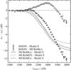 |
Fig. 1 Frequency differences between BiSON observations of low-degree solar oscillations and Model S before (grey points) and after (white points) the near-surface layers are replaced by the profile of the G2-type MURaM simulation averaged over time and surfaces of constant geometric depth. The solid line shows the difference between the frequencies before and after replacing the near-surface layers. In addition, the dotted and dashed lines show the frequency differences when the MURaM simulation is instead averaged over surfaces of constant pressure P or optical depth τ. With the averaged MURaM profile, the residual frequency difference is reduced to at most about 3 μHz. The frequency changes are sensitive to the averaging method at about the 1 μHz level, which is smaller than the surface effect itself. |
Though the MURaM simulation and Model S have not been calibrated to each other, both match the same deeper, near-adiabatic structure of the Sun. In solar-calibrated stellar models like Model S, the choice of mixing-length parameter fixes the entropy jump across the near-surface superadiabatic layer and, consequently, also fixes the adiabat of the deep convection zone (Gough & Weiss 1976). The MURaM simulation is sufficiently realistic that, given the Sun’s effective temperature, surface gravity and composition, the same adiabat is recovered.
The dotted and dashed curves in Fig. 1 show the frequency changes induced by instead replacing the near-surface layers with the simulation data averaged at constant pressure or optical depth. The variation in the surface term shows that there is some uncertainty induced by the averaging process, but this uncertainty is smaller than the overall scale of the frequency changes. For the rest of the paper, all averages of simulation properties were taken at constant geometric depth.
Parameters of the MURaM simulations and MESA models along with best-fitting parameters for analytic corrections available in the literature.
Figure 2 shows the differences in the Brunt–Väisälä frequency N2 and sound speed cs at the matching point. Though the change in the Brunt–Väisälä is fractionally large, the matching point is inside the convection zone, where N2 is negative. The mode frequencies are large and apparently unaffected, though this would not be the case for non-radial modes in more evolved stars. The fractional sound speed difference is less than 0.2 per cent.
The change in the frequencies caused only by the modification of the equilibrium stellar structure is just one of the many causes of the surface effect. As noted in the extensive discussion by Rosenthal (1997), it is difficult to predict how these many effects will combine to give precisely the correct surface term, but this does not mean that it is not worth studying the individual effects in isolation. Thus, the results here should be interpreted with the caveat that they are only one component of the surface effect and have been computed in a simplified fashion.
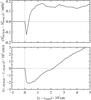 |
Fig. 2 Structural differences between the patched and unpatched models near the matching point. The upper panel shows differences in the Brunt–Väisälä frequency while the lower panel shows differences in the sound speed. |
Motivated by the positive result for the Sun, we computed stellar models to match the properties of four of the simulations by Beeck et al. (2013) in the same way, listed in Table 1, and computed the change in mode frequencies induced by replacing the surface layers with the averaged simulation data. We present here a preliminary exploration of how the surface effect varies with spectral type on the main sequence, based on these simulations. This is the same procedure as followed in the recent results by Sonoi et al. (2015). Their models A and B have similar atmospheric parameters to our G2 and F3 simulations. Their other models extend to more evolved stars, whereas ours extend to cooler main-sequence stars. In Sect. 2, we briefly describe the simulations, the stellar models and how we matched them. In Sect. 3, we present the frequency shifts and compare them with several parametric fits in the literature, before concluding in Sect. 4.
2. Methods
2.1. MURaM models
The simulations of the near-surface convection used in this work were computed by Beeck et al. (2013), to which the reader is referred for additional details and references about the simulations and the code used to produce them, MURaM. In short, MURaM is a three-dimensional, time-dependent, compressible radiative magnetohydrodynamics (MHD) code, developed jointly by groups at the University of Chicago and the Max Planck Institute for Solar System Research (Vögler et al. 2005). The non-grey radiation transport scheme is based on the method of short characteristics (Kunasz & Auer 1988) and uses opacity binning (Nordlund 1982) based on opacity distribution functions from ATLAS9 (Kurucz 1993). The code uses the OPAL equation of state (Rogers et al. 1996) with the solar composition of Anders & Grevesse (1989).
The three-dimensional, time-dependent simulations were averaged over time and at constant geometric depth z (where z = 0 corresponds to the average depth of the τ ≈ 1 surface) to produce one-dimensional profiles of density, pressure and sound speed as functions of depth. This is a simplification: it is not known how to correctly average the fluid such that the average oscillations are reproduced. The averaged simulation profiles were then used to replace the near-surface layers of the stellar models, described below. Specifically, we used profiles for the averaged pressure, density (and their gradients, computed from finite differences of their logarithms) and sound speed as functions of depth. This implies that although the MURaM simulations at a given point and time satisfy the same equation of state as the stellar models, the averages do not. The adiabatic index was computed from the sound speed, so that although this adiabatic index is not the same as the simulation average, it reproduces the average sound speed for the oscillation calculation. Finally, the Brunt-Väisälä frequency was computed from the adiabatic index, pressure gradient and density gradient. Like Sonoi et al. (2015), we assumed that the relative Lagrangian perturbation to the turbulent pressure is the same as that of the gas pressure, which Rosenthal et al. (1999) referred to as the “gas Γ1 approximation”.
2.2. MESA models
Stellar models were computed using the Modules for Experiments in Stellar Astrophysics (MESA2, revision 7624, Paxton et al. 2011, 2013, 2015). As far as was possible, we used default options for the stellar models. Each model was initialized on the pre-main-sequence with uniform composition and central temperature 9 × 10⁵K and evolved until either hydrogen was exhausted at the centre or χ2 had increased to more than 100 times the minimum value for that run (see below for how χ2 was defined). The overall metallicity (i.e. Z/X) and metal mixture of the stellar models was chosen to be that of Anders & Grevesse (1989) to match the composition of the MURaM simulations. We used a helium abundance of 0.27431. To ensure that the surface composition matched the simulations, atomic diffusion and extra mixing were not included. Opacities were taken from the OPAL tables (Iglesias & Rogers 1996) and Ferguson et al. (2005) at high and low temperatures, respectively. The opacity tables were computed with the nearest available solar mixture, that of Grevesse & Noels (1993). The equation of state tables are based on the 2005 update to the OPAL tables (Rogers & Nayfonov 2002). Nuclear reaction rates are taken from the NACRE compilation (Angulo et al. 1999) or, if not available there, from Caughlan & Fowler (1988). Convection was described using mixing-length theory (Böhm-Vitense 1958). We used an Eddington grey atmosphere at the surface boundary, integrated to an optical depth of τ = 10-4.
2.3. Fitting method
For each simulation, we first matched stellar models with six mixing length parameters α to the simulation’s Teff and log g using the downhill simplex (Nelder & Mead 1965) optimization implemented in MESA. We optimized the masses and ages for models with fixed mixing-length parameters α between 1.5 and 2.0 in steps of 0.1. The objective function was a standard χ2, with the uncertainty on Teff taken as the rms variation of the temperature listed by Beeck et al. (2013), and the uncertainty in log g set to 0.001 dex. Because we optimized two parameters (mass and age) for two observations (Teff and log g), the choice of uncertainties is in essence arbitrary.
We then patched the averaged MURaM profiles onto the stellar models by finding the depth at which the pressure of the stellar model matched the pressure at the base of the MURaM profile, and replacing the stellar model data with the averaged data from the simulation. We inspected the difference between the densities at the matching point, and computed additional stellar models with intermediate mixing-length parameters until a sufficiently accurate match was found. As a cross-check, we inspected the sound speed profile to ensure that it too was sufficiently smooth. The best-fitting values of α are also listed in Table 1. With this procedure, we calibrated α to a precision of about 0.01.
The best-fitting model of type K5 has a lower mixing-length parameter α than the other simulations. This goes against trends determined by matching 1D mixing-length theory atmospheres to 2D and 3D simulations (e.g. Ludwig et al. 1999; Trampedach et al. 2014b). Though we have not found an obvious explanation for this, we note that the convective envelope in the stellar model extends above the photosphere, but the photosphere boundary condition assumes that the luminosity is transported only by radiation. In addition, this stellar model is so young that it still has a residual convective core from its pre-main-sequence contraction. Regardless of the unexpectedly low mixing-length parameter, we confirmed that the structure of the K5 stellar model matches the simulation profile in its deepest layers, as for the other three stellar types.
The process above gave us two models for each spectral type: the original stellar model and the patched model, where the near-surface layers were replaced by the averaged MURaM simulations. Both models share the same internal structure below the matching point and therefore have the same luminosity, but the patched models have slightly larger radii and lower surface temperatures. We computed the adiabatic oscillation frequencies for both models using ADIPLS (Christensen-Dalsgaard 2008) and took the frequency shift as the difference between the frequencies for modes found for both models. The process is similar in spirit to the study by Piau et al. (2014) but we have neither incorporated information from the MURaM simulations into the stars’ evolution nor considered the effects of magnetic fields. Our method is in essence identical to the method of Sonoi et al. (2015) though we have used low-degree modes up to ℓ = 3, whereas they restricted themselves to radial modes.
We close by noting that it is possible to compute the frequency shifts from structure kernels by treating the differences between the patched models and the original stellar models as a structural perturbation. Given that the fractional structure differences are large, quantitative results are questionable. Nevertheless, we performed this calculation for Model S, treating the differences as sound speed and density perturbations, and obtained qualitatively similar results, dominated by the density perturbation.
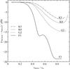 |
Fig. 3 Frequency differences between the stellar models and patched models computed for all four simulations, with the horizontal axis rescaled by the acoustic cut-off frequency νac. The shapes of the frequency differences as a function of frequency are similar for the three cooler simulations (G2, K0 and K5), whereas the difference for the F3 simulation is more complicated. |
3. Results
3.1. Overall features
Figure 3 shows the frequency differences as a function of frequency for all four simulations, with the frequencies divided by the acoustic cut-off frequency νac. All the surface effects are negative in sign at high frequencies, as for the Sun, in the sense that stellar models overpredict the mode frequencies. In addition, the overall scale of the surface effect decreases with decreasing effective temperature. There is also a clear change around 0.3 νac, below which the surface effect is smaller than about 1 μHz across all the stars. Christensen-Dalsgaard & Thompson (1997) showed that this is caused by the near-cancellation of different contributions to Eulerian surface perturbations. Lagrangian perturbations are confined closer to the surface, above the upper turning point of the low-frequency modes.
The surface effects in the three cooler spectral types (G2, K0 and K5) are similar in shape. The largest absolute differences occur at decreasing relative frequency because of the shape of the mode inertia curve. That is, as the temperatures decrease, the minimum mode inertia occurs at slightly lower relative frequency. As expected, the results depend on the choice of underlying stellar model, since the surface shift in the calibrated G2 model differs by up to 5 μHz compared to the frequency shift computed for Model S.
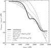 |
Fig. 4 Frequency differences between a stellar model calibrated to the F3 simulation, and the patched model, in which the near-surface layers were replaced by the averaged simulation profile. Additional curves show the parametric fits of the one-term correction by Ball & Gizon (2014; dashed), their two-term fit (dotted), a power law (dot-dot-dashed), the modified Lorentzian of Sonoi et al. (2015; long-dashed), and a scaled solar correction (dot-dashed). The two-term fit is clearly better able to capture the distinct shape of the frequency difference. |
The shape of the surface effect in the F3 model is notably different, showing multiple bends as a function of frequency. This is mostly because the mode inertiae are a more complicated function of frequency. The bend in the surface effect around −17 μHz corresponds to the first minimum of the mode inertiae, and the additional bend around −30 μHz corresponds similarly to a second minimum. The patched model also shows a jump in Γ1 of about 0.02 at the matching point because helium is partially ionized at the base of the MURaM simulation. Such abrupt changes in the stellar structure, known as “acoustic glitches” (e.g. Houdek & Gough 2007), create features in the frequencies that oscillate as a function of frequency. In this case, however, it appears that the shape of the mode inertia curve dominates the change in the frequencies. This is made clearer by the parametric fits in Sect. 3.2.
Though already widely accepted, the shapes of the frequency differences confirm that most of the modes observed in main-sequence solar-like oscillators of all spectral types are affected by surface effects. The frequency at which maximum oscillation power is observed, known as νmax, is roughly 0.6 νac, with a typical FWHM of about half of νmax (i.e. 0.3 νac, Chaplin et al. 2011). Hence, our results confirm that one should expect surface effects to affect all modes observed within one FWHM of the power envelope. This motivates observations using line-of-sight velocities, for which the background signal of granulation is much weaker and the lower-frequency modes are easier to detect. Such observations will hopefully become possible as the Stellar Oscillation Network Group (SONG, Grundahl et al. 2014) increases its capacity.
3.2. Comparison with parametric fits
In principle, the surface effects computed here can be used to calibrate parametric fits available in the literature, but the coverage in the Hertzsprung–Russell diagram (only four points) is presently too sparse to make thorough inferences. However, we can compute the best-fitting parameters for these analytic models, partly to subsequently compare with fits to real stars with similar parameters, and partly to compare which prescriptions fit our results better. The latter approach is similar to the recent work by Schmitt & Basu (2015), who computed theoretical frequency shifts using structure kernels, except that here we are using the simulation data. Sonoi et al. (2015) also compared parametric fits but limited their comparison to the power law proposed by Kjeldsen et al. (2008) and their own modified Lorentzian parametrization.
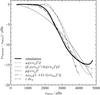 |
Fig. 5 As in Fig. 4, but for the G2 star. The two-term fit is nearly perfect across the whole frequency range. |
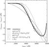 |
Fig. 6 As in Fig. 4, but for the K0 star. The two-term fit again fits best, but the modified Lorentzian and the scaled solar correction also reproduce the shift reasonably well. |
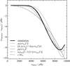 |
Fig. 7 As in Fig. 4, but for the K5 star. As for the K0 star, the two-term fit, modified Lorentzian and scaled solar correction match quite well. |
Figures 4–7 show the predicted surface effects in the F3, G2, K0 and K5 models, along with parametric fits from several sources. Each parametric form specifies the difference between the model frequency νmdl and the corrected frequency νcor as some function of the model frequency and sometimes mode inertia ℐ, normalized to the total displacement at the photosphere.
First, there are the two fits presented by Ball & Gizon (2014). They proposed either a one-term fit, 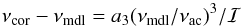 (1)or two-term fit,
  (2)where a3, b-1 and b3 are coefficients that minimize the difference between a model and whatever observations are being fit. Here, the acoustic cut-off frequency νac is used purely to scale the frequencies.
Second, there is the power-law fit suggested by Kjeldsen et al. (2008),  (3)Those authors proposed that p1 (originally denoted b) be calibrated to the Sun and p0 calibrated using the modelled and observed large separations, based on homology arguments. Here, we optimize the values of both to see how they vary, and use the acoustic cut-off as the reference frequency νref.
Third, there is the modified Lorentzian suggested by Sonoi et al. (2015), 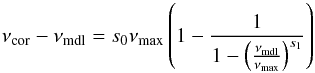 (4)where the frequency of maximum oscillation power νmax is determined from the scaling relation (Kjeldsen & Bedding 1995)
 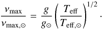 (5)The free parameters s0 and s1 correspond to the parameters α and β in the original work by Sonoi et al. (2015).
Finally, we include a scaled solar correction, computed as described by Schmitt & Basu (2015). Our solar correction was taken as the difference between Model S and the low-frequency BiSON data, indicated in Fig. 1. We note that including a constant offset does not make sense, since it is clear that the low-frequency modes are not shifted at all in our results. We fit all of the coefficients using non-linear least squares without weighting any of the frequencies.
The best-fitting parameters are presented with the corresponding models in Table 1. Though we refrain from concluding anything quantitative from the unweighted residuals, it is still useful to inspect the quality of the fits. Figures 4–7 show that the two-term fit by Ball & Gizon (2014) overall fits the simulations better than the other corrections, notably including the F3 simulation. For the F3 simulation, it is important to include the mode inertiae in the fitting formula to correctly recover the distinct shape of the surface effect.
The scaled solar surface term performs well in the cooler stars, where it reproduces the initial increase in the surface term quite well. However, because the solar surface term is scaled by mean density (or the large separation) rather than the acoustic cut-off frequency, a shrinking frequency range is covered as the temperature decreases. The modified Lorentzian is also generally able to reproduce the initial rise in the magnitude of the surface term as a function of frequency. In the F3 model, neither the scaled solar correction nor the modified Lorentzian are able to match the surface term’s more complicated shape. For the G2 and F3 simulations, the parameter values of the modified Lorentzian compare well with the fits by Sonoi et al. (2015) to their corresponding models A and B.
The power law clearly misses the distinct shape of the F3 simulation, but also fails to reproduce the sharp increase and ultimate decrease of the surface effect in the cooler stars. We note that, to reduce the error at high frequency, the indices of the power laws are all much lower (around 2) than typical values used in the correction by Kjeldsen et al. (2008) (usually between about 4.5 and 5.5), but reasonably consistent for all four spectral types.
For the sake of comparison, we have included in Table 1 the results of calibrating the surface corrections to the frequency differences between Model S and the low-degree BiSON observations (i.e. the grey points in Fig. 1). The overall magnitudes of the surface terms are consistent with our results for the fitted stellar models, though the result for the power law is markedly different. There are many potential reasons for slight differences in the observed and modelled surface terms but the most important is that we have only regarded the static structural effect of the surface term. The frequency differences between Model S and the BiSON observations necessarily include all the physical processes that contribute to the surface effect (see Sect. 1).
4. Conclusion
We have used profiles from averaging 3D radiation hydrodynamic simulations over time and space for four spectral types to compute corrections to stellar oscillation frequencies induced by better modelling the equilibrium structure of the near-surface layers of solar-like oscillators: a component of the so-called “surface effect”. In the three cooler simulations (types G2, K0 and K5), the surface effects are similar in shape to what is already known from differences between solar observations and models calibrated to the match the observed solar luminosity and radius at the meteoritic age of the solar system. The hotter simulation, of a star of spectral type F3, predicts a qualitatively different surface effect. Across the four cases, the surface effect consistently decreases in magnitude with decreasing effective temperature. In other words, our results suggest that hotter main-sequence stars have larger surface effects.
By comparing parametric fits available in the literature, we find that the two-term fit by Ball & Gizon (2014) is best able to reproduce the frequency shifts, though the scaled solar term performs comparably well in the solar-type and cooler stars. Thus, we corroborate the conclusion of Schmitt & Basu (2015), who modelled surface effects using structural perturbations.
Our derived frequency difference generally agrees with the recent results by Sonoi et al. (2015), who in essence performed the same calculation for a different range of stellar parameters using different modelling codes. Our G2 and F3 simulations are similar to their models A and B, and our derived frequency differences are qualitatively and quantitatively very similar. Their models generally explored lower surface gravities, whereas our K0 and K5 simulations extend the results to cooler main-sequence stars. Our methods thus corroborate their results where they overlap, and complement them elsewhere. Sonoi et al. (2015) did not fit the parametrizations of Ball & Gizon (2014) and concluded that their modified Lorentzian is superior to the power law of Kjeldsen et al. (2008). Our results support this conclusion but find that the combined correction of Ball & Gizon (2014) is even better, mostly because it incorporates the mode inertiae.
This preliminary study exploits simulation data that was serendipitously created for other purposes. The obvious next step is to compute further simulations specifically to be matched to stellar models. In addition, we intend to explore automatic calibration of the models to the averaged simulation profiles, rather than matching the surface properties and manually adjusting the mixing-length parameter to obtain a good fit at the base of the MURaM simulations.
We close by noting that our results only treat one structural component of the surface effect. That is, we have only computed frequency shifts caused by simplified modelling of the static, equilibrium state of the near-surface layers. These results have no bearing on the effects caused by ignoring non-adiabatic effects on the oscillation modes, perturbations to the turbulent pressure, or small- or large-scale flows. Any of the other components may induce surface effects that vary differently between different stars and, taken together, produce trends that differ from what we have found. However, as is clear from the solar case, the structural effect is a major contributor and this work thus offers insight into how the surface effect varies across the main sequence.
Here, we define the acoustic cut-off frequency to be the maximum of cs/ 4πHP, where cs is the sound speed and HP is the pressure scale height.
Acknowledgments
The authors acknowledge research funding by Deutsche Forschungsgemeinschaft (DFG) under grant SFB 963/1 “Astrophysical flow instabilities and turbulence”, Projects A18 (WHB) and A16 (BB and RHC). L.G. acknowledges support by the Center for Space Science at the NYU Abu Dhabi Institute under grant G1502. We are grateful to Aaron Birch and Hans-Günter Ludwig for helpful comments on the results and manuscript.
References
- Anders, E., & Grevesse, N. 1989, Geochim. Cosmochim. Acta, 53, 197 [Google Scholar]
- Angulo, C., Arnould, M., Rayet, M., et al. 1999, Nucl. Phys. A, 656, 3 [NASA ADS] [CrossRef] [Google Scholar]
- Auvergne, M., Bodin, P., Boisnard, L., et al. 2009, A&A, 506, 411 [NASA ADS] [CrossRef] [EDP Sciences] [Google Scholar]
- Ball, W. H., & Gizon, L. 2014, A&A, 568, A123 [NASA ADS] [CrossRef] [EDP Sciences] [Google Scholar]
- Beeck, B., Cameron, R. H., Reiners, A., & Schüssler, M. 2013, A&A, 558, A48 [NASA ADS] [CrossRef] [EDP Sciences] [Google Scholar]
- Bhattacharya, J., Hanasoge, S., & Antia, H. M. 2015, ApJ, 806, 246 [NASA ADS] [CrossRef] [Google Scholar]
- Böhm-Vitense, E. 1958, Z. Astrophys., 46, 108 [Google Scholar]
- Borucki, W. J., Koch, D., Basri, G., et al. 2010, Science, 327, 977 [NASA ADS] [CrossRef] [PubMed] [Google Scholar]
- Broomhall, A.-M., Chaplin, W. J., Davies, G. R., et al. 2009, MNRAS, 396, L100 [NASA ADS] [CrossRef] [Google Scholar]
- Brown, T. M. 1984, Science, 226, 687 [NASA ADS] [CrossRef] [PubMed] [Google Scholar]
- Caughlan, G. R., & Fowler, W. A. 1988, Atomic Data and Nuclear Data Tables, 40, 283 [Google Scholar]
- Chaplin, W. J., Kjeldsen, H., Bedding, T. R., et al. 2011, ApJ, 732, 54 [NASA ADS] [CrossRef] [Google Scholar]
- Christensen-Dalsgaard, J. 2008, Ap&SS, 316, 113 [NASA ADS] [CrossRef] [Google Scholar]
- Christensen-Dalsgaard, J., & Thompson, M. J. 1997, MNRAS, 284, 527 [NASA ADS] [Google Scholar]
- Christensen-Dalsgaard, J., Dappen, W., Ajukov, S. V., et al. 1996, Science, 272, 1286 [CrossRef] [Google Scholar]
- Davies, G. R., Chaplin, W. J., Elsworth, Y., & Hale, S. J. 2014, MNRAS, 441, 3009 [NASA ADS] [CrossRef] [Google Scholar]
- Ferguson, J. W., Alexander, D. R., Allard, F., et al. 2005, ApJ, 623, 585 [NASA ADS] [CrossRef] [Google Scholar]
- Goldreich, P., Murray, N., Willette, G., & Kumar, P. 1991, ApJ, 370, 752 [NASA ADS] [CrossRef] [Google Scholar]
- Gough, D. O., & Weiss, N. O. 1976, MNRAS, 176, 589 [Google Scholar]
- Grevesse, N., & Noels, A. 1993, in Origin and Evolution of the Elements, eds. N. Prantzos, E. Vangioni-Flam, & M. Casse, 15 [Google Scholar]
- Grundahl, F., Christensen-Dalsgaard, J., Pallé, P. L., et al. 2014, in IAU Sym. 301, eds. J. A. Guzik, W. J. Chaplin, G. Handler, & A. Pigulski, 69 [Google Scholar]
- Hanasoge, S. M., Gizon, L., & Bal, G. 2013, ApJ, 773, 101 [NASA ADS] [CrossRef] [Google Scholar]
- Houdek, G., & Gough, D. O. 2007, MNRAS, 375, 861 [NASA ADS] [CrossRef] [Google Scholar]
- Iglesias, C. A., & Rogers, F. J. 1996, ApJ, 464, 943 [NASA ADS] [CrossRef] [Google Scholar]
- Kjeldsen, H., & Bedding, T. R. 1995, A&A, 293, 87 [NASA ADS] [Google Scholar]
- Kjeldsen, H., Bedding, T. R., & Christensen-Dalsgaard, J. 2008, ApJ, 683, L175 [NASA ADS] [CrossRef] [Google Scholar]
- Kunasz, P., & Auer, L. H. 1988, J. Quant. Spec. Radiat. Transf., 39, 67 [NASA ADS] [CrossRef] [Google Scholar]
- Kurucz, R. L. 1993, SYNTHE spectrum synthesis programs and line data (Cambridge, MA: Smithsonian Astophysical Observatory) [Google Scholar]
- Libbrecht, K. G., & Woodard, M. F. 1990, Nature, 345, 779 [Google Scholar]
- Ludwig, H.-G., Freytag, B., & Steffen, M. 1999, A&A, 346, 111 [NASA ADS] [Google Scholar]
- Ludwig, H.-G., Caffau, E., Steffen, M., et al. 2009, Mem. Soc. Astron. It., 80, 711 [NASA ADS] [Google Scholar]
- Murawski, K., & Roberts, B. 1993a, A&A, 272, 595 [NASA ADS] [Google Scholar]
- Murawski, K., & Roberts, B. 1993b, A&A, 272, 601 [NASA ADS] [Google Scholar]
- Nelder, J. A., & Mead, R. 1965, The Computer Journal, 7, 308 [Google Scholar]
- Nordlund, A. 1982, A&A, 107, 1 [NASA ADS] [Google Scholar]
- Paxton, B., Bildsten, L., Dotter, A., et al. 2011, ApJS, 192, 3 [Google Scholar]
- Paxton, B., Cantiello, M., Arras, P., et al. 2013, ApJS, 208, 4 [NASA ADS] [CrossRef] [Google Scholar]
- Paxton, B., Marchant, P., Schwab, J., et al. 2015, ApJS, 220, 15 [Google Scholar]
- Piau, L., Collet, R., Stein, R. F., et al. 2014, MNRAS, 437, 164 [NASA ADS] [CrossRef] [Google Scholar]
- Rogers, F. J., & Nayfonov, A. 2002, ApJ, 576, 1064 [Google Scholar]
- Rogers, F. J., Swenson, F. J., & Iglesias, C. A. 1996, ApJ, 456, 902 [NASA ADS] [CrossRef] [Google Scholar]
- Rosenthal, C. S. 1997, in SCORe’96 : Solar Convection and Oscillations and their Relationship, eds. F. P. Pijpers, J. Christensen-Dalsgaard, & C. S. Rosenthal, Astrophys. Space Sci. Libr., 225, 145 [Google Scholar]
- Rosenthal, C. S., Christensen-Dalsgaard, J., Nordlund, Å., Stein, R. F., & Trampedach, R. 1999, A&A, 351, 689 [NASA ADS] [Google Scholar]
- Schlattl, H., Weiss, A., & Ludwig, H.-G. 1997, A&A, 322, 646 [NASA ADS] [Google Scholar]
- Schmitt, J. R., & Basu, S. 2015, ApJ, 808, 123 [NASA ADS] [CrossRef] [Google Scholar]
- Sonoi, T., Samadi, R., Belkacem, K., et al. 2015, A&A, 583, A112 [NASA ADS] [CrossRef] [EDP Sciences] [Google Scholar]
- Trampedach, R., Asplund, M., Collet, R., Nordlund, Å., & Stein, R. F. 2013, ApJ, 769, 18 [NASA ADS] [CrossRef] [Google Scholar]
- Trampedach, R., Stein, R. F., Christensen-Dalsgaard, J., Nordlund, Å., & Asplund, M. 2014a, MNRAS, 442, 805 [NASA ADS] [CrossRef] [Google Scholar]
- Trampedach, R., Stein, R. F., Christensen-Dalsgaard, J., Nordlund, Å., & Asplund, M. 2014b, MNRAS, 445, 4366 [NASA ADS] [CrossRef] [Google Scholar]
- Vögler, A., Shelyag, S., Schüssler, M., et al. 2005, A&A, 429, 335 [NASA ADS] [CrossRef] [EDP Sciences] [Google Scholar]
All Tables
Parameters of the MURaM simulations and MESA models along with best-fitting parameters for analytic corrections available in the literature.
All Figures
|
Fig. 1 Frequency differences between BiSON observations of low-degree solar oscillations and Model S before (grey points) and after (white points) the near-surface layers are replaced by the profile of the G2-type MURaM simulation averaged over time and surfaces of constant geometric depth. The solid line shows the difference between the frequencies before and after replacing the near-surface layers. In addition, the dotted and dashed lines show the frequency differences when the MURaM simulation is instead averaged over surfaces of constant pressure P or optical depth τ. With the averaged MURaM profile, the residual frequency difference is reduced to at most about 3 μHz. The frequency changes are sensitive to the averaging method at about the 1 μHz level, which is smaller than the surface effect itself. |
| In the text | |
|
Fig. 2 Structural differences between the patched and unpatched models near the matching point. The upper panel shows differences in the Brunt–Väisälä frequency while the lower panel shows differences in the sound speed. |
| In the text | |
|
Fig. 3 Frequency differences between the stellar models and patched models computed for all four simulations, with the horizontal axis rescaled by the acoustic cut-off frequency νac. The shapes of the frequency differences as a function of frequency are similar for the three cooler simulations (G2, K0 and K5), whereas the difference for the F3 simulation is more complicated. |
| In the text | |
|
Fig. 4 Frequency differences between a stellar model calibrated to the F3 simulation, and the patched model, in which the near-surface layers were replaced by the averaged simulation profile. Additional curves show the parametric fits of the one-term correction by Ball & Gizon (2014; dashed), their two-term fit (dotted), a power law (dot-dot-dashed), the modified Lorentzian of Sonoi et al. (2015; long-dashed), and a scaled solar correction (dot-dashed). The two-term fit is clearly better able to capture the distinct shape of the frequency difference. |
| In the text | |
|
Fig. 5 As in Fig. 4, but for the G2 star. The two-term fit is nearly perfect across the whole frequency range. |
| In the text | |
|
Fig. 6 As in Fig. 4, but for the K0 star. The two-term fit again fits best, but the modified Lorentzian and the scaled solar correction also reproduce the shift reasonably well. |
| In the text | |
|
Fig. 7 As in Fig. 4, but for the K5 star. As for the K0 star, the two-term fit, modified Lorentzian and scaled solar correction match quite well. |
| In the text | |
Current usage metrics show cumulative count of Article Views (full-text article views including HTML views, PDF and ePub downloads, according to the available data) and Abstracts Views on Vision4Press platform.
Data correspond to usage on the plateform after 2015. The current usage metrics is available 48-96 hours after online publication and is updated daily on week days.
Initial download of the metrics may take a while.