| Issue |
A&A
Volume 592, August 2016
|
|
|---|---|---|
| Article Number | A64 | |
| Number of page(s) | 12 | |
| Section | Extragalactic astronomy | |
| DOI | https://doi.org/10.1051/0004-6361/201527063 | |
| Published online | 25 July 2016 | |
Disk galaxy scaling relations at intermediate redshifts
I. The Tully-Fisher and velocity-size relations⋆,⋆⋆
1 Institute for Astro- and Particle Physics, Technikerstrasse 25/8, 6020 Innsbruck, Austria
e-mail: asmus.boehm@uibk.ac.at
2 Institute of Astronomy, Türkenschanzstrasse 17, 1180 Vienna, Austria
Received: 27 July 2015
Accepted: 17 May 2016
Aims. Galaxy scaling relations such as the Tully-Fisher relation (between the maximum rotation velocity Vmax and luminosity) and the velocity-size relation (between Vmax and the disk scale length) are powerful tools to quantify the evolution of disk galaxies with cosmic time.
Methods. We took spatially resolved slit spectra of 261 field disk galaxies at redshifts up to z ≈ 1 using the FORS instruments of the ESO Very Large Telescope. The targets were selected from the FORS Deep Field and William Herschel Deep Field. Our spectroscopy was complemented with HST/ACS imaging in the F814W filter. We analyzed the ionized gas kinematics by extracting rotation curves from the two-dimensional spectra. Taking into account all geometrical, observational, and instrumental effects, these rotation curves were used to derive the intrinsic Vmax.
Results. Neglecting galaxies with disturbed kinematics or insufficient spatial rotation curve extent, Vmax was reliably determined for 124 galaxies covering redshifts 0.05 < z < 0.97. This is one of the largest kinematic samples of distant disk galaxies to date. We compared this data set to the local B-band Tully-Fisher relation and the local velocity-size relation. The scatter in both scaling relations is a factor of ~2 larger at z ≈ 0.5 than at z ≈ 0. The deviations of individual distant galaxies from the local Tully-Fisher relation are systematic in the sense that the galaxies are increasingly overluminous toward higher redshifts, corresponding to an overluminosity ΔMB = −(1.2 ± 0.5) mag at z = 1. This luminosity evolution at given Vmax is probably driven by younger stellar populations of distant galaxies with respect to their local counterparts, potentially combined with modest changes in dark matter mass fractions. The analysis of the velocity-size relation reveals that disk galaxies of a given Vmax have grown in size by a factor of ~1.5 over the past ~8 Gyr, most likely through accretion of cold gas and/or small satellites. From scrutinizing the combined evolution in luminosity and size, we find that the galaxies that show the strongest evolution toward smaller sizes at z ≈ 1 are not those that feature the strongest evolution in luminosity, and vice versa.
Key words: galaxies: spiral / galaxies: evolution / galaxies: kinematics and dynamics / galaxies: structure
Based on observations with the European Southern Observatory Very Large Telescope (ESO-VLT), observing run IDs 65.O-0049, 66.A-0547, 68.A-0013, 69.B-0278B, 70.B-0251A and 081.B-0107A.
The full Table 1 is only available at the CDS via anonymous ftp to cdsarc.u-strasbg.fr (130.79.128.5) or via http://cdsarc.u-strasbg.fr/viz-bin/qcat?J/A+A/592/A64
© ESO, 2016
1. Introduction
Observational studies of galaxy evolution have made great progress in the past decade. In the course of some projects, redshifts and spectral energy distributions of several 104 galaxies at significant cosmological look-back times were gained – two examples are the VVDS (Le Fèvre et al. 2005) and zCOSMOS (Lilly et al. 2007) surveys. Other projects focused on smaller samples to conduct detailed studies of the scaling relations that link fundamental structural and kinematical parameters of galaxies. The most famous scaling relation for spirals is the Tully-Fisher relation (TFR, Tully & Fisher 1977), which relates the luminosity to the maximum rotation velocity Vmax. Equivalents of the classical, that is, of the optical TFR were established later, showing that the stellar mass M∗ (e.g., Bell & de Jong 2001) or total baryonic mass (i.e., stars and gas, e.g. McGaugh et al. 2000) also correlate with Vmax. In this sense, the optical TFR is only a variant of a more fundamental relation between the baryonic and the dark matter content of disk galaxies. Since dark matter dominates the total mass budget, Vmax can be used to estimate the dark matter halo mass (e.g., Mo et al. 1998). In addition to luminosity, stellar, or baryonic mass, the disk scale length is also correlated with Vmax (e.g., Mao et al. 1998); this is referred to as the rotation velocity-size relation (VSR). The three parameters Vmax, size, and luminosity span a parameter space in which disks populate a two-dimensional plane with small intrinsic scatter. Burstein et al. (1997), for instance, used this parameter space with sizes given as effective radii, and Koda et al. (2000) carried out a similar investigation using the disk isophotal radius at μI = 23.5 mag. The distribution of late-type galaxies within a plane in this parameter space is similar to the fundamental plane that is valid for early-type galaxies (e.g., Dressler et al. 1987).
The first observational attempts to construct the optical TFR of distant spirals and to quantify their evolution in luminosity were made almost two decades ago by Vogt et al. (1996) and Rix et al. (1997), for example. For many of the following years, discrepant results have been published from different studies on a possible evolution of the Tully-Fisher relation with cosmic time in zero point or slope. Vogt (2001) did not find any evolution of the B-band TFR up to redshifts z ≈ 1, while Böhm et al. (2004), Bamford et al. (2006), or Fernàndez Lorenzo (2010), for example, found that disk galaxies at z ≈ 1 were brighter by ΔMB ≈ −1 mag for a given maximum rotation velocity. Böhm et al. also discussed a possible slope change with cosmic time in the sense that the luminosity evolution of low-mass spirals was stronger than that of high-mass ones. Weiner at al. (2006), on the other hand, found the opposite evolution: a stronger brightening in high-mass disk galaxies. Böhm & Ziegler (2007) showed that a strong evolution of the TFR scatter could mimic an evolution in TFR slope through selection effects. Kassin et al. (2007) established that even galaxies with kinematic disturbances, which usually do not follow the classical TFR, obey a remarkably tight correlation when non-ordered motions are taken into account. To this end, these authors introduced the parameter S0.5 that combines Vmax and gas velocity dispersion, finding a constant slope over the epoch 0.1 < z < 1.2.
Only more recently has there been growing consent that the local TFR slope holds at least up to redshifts of about unity for all variants of the TFR. Some of these studies were like all of the projects mentioned above based on slit spectroscopy (e.g. Fernàndez Lorenzo et al. 2010; Miller et al. 2011), others made use of integral field units (IFUs, e.g., Flores et al. 2006; Puech et al. 2008). As a result of the time-expensive approach, samples constructed using IFUs are usually smaller than slit-based ones. The gain is a direct observability of (at least part of) the two-dimensional rotation velocity field. Mismatches between photometric and kinematic center, or photometric and kinematic position angle, can only be detected with this type of data.
Toward high redshifts z > 1, IFUs are a necessity because interaction and merger events were much more frequent at these epochs. In effect, many high-z star-forming galaxies feature complex or disturbed kinematics. Several surveys have been conducted with the adaptive-optics-assisted SINFONI instrument of the ESO Very Large Telescope: AMAZE (Maiolino et al. 2008), SINS (Förster-Schreiber et al. 2009), and MASSIV (Epinat et al. 2009). Based on data from MASSIV, for instance, Vergani et al. (2012) found only a small increase in stellar mass (~0.15 dex on average, depending on the reference sample at z = 0) between z ≈ 1.2 and the present-day universe, at fixed Vmax. Gnerucci et al. (2011) investigated 11 disks at z ≈ 3 from the AMAZE data set, finding stellar masses lower than local masses by ~1 dex. However, even for this sample of regularly rotating disks, a very large scatter was observed, and the authors concluded that the TFR is not yet established at that cosmic epoch. Cresci et al. (2009), on the other hand, found a much smaller evolution of 0.41 dex in log M∗ since z ≈ 2.2 using SINS data.
A potential environmental dependence of the TFR has been subject of many studies. Several authors found that field and cluster samples have the same TFR slope, but the scatter is increased in dense environments (e.g., Moran et al. 2007; Bösch et al. 2013b). This is probably induced by cluster-specific interaction processes. Tidal interactions between close galaxies can increase the star formation rate (e.g., Lambas et al. 2003), whereas interactions between the interstellar medium and the hot intra-cluster medium (ram-pressure stripping) can push gas out of a disk galaxy and in the extreme case totally quench star formation (e.g., Quilis et al. 2000). These mechanisms lead to a wider range in luminosities at given Vmax and increase the fraction of perturbed gas kinematics (e.g., Bösch et al. 2013a). In turn, Vmax measurements in dense environments carry larger systematic errors. All these effects are likely to contribute to the larger TFR scatter found in clusters. However, the situation changes when field and cluster samples are matched in rotation curve quality, that is, when galaxies are rejected that have perturbed kinematics due to cluster-specific interactions. It was found that the distributions of field and cluster samples then are very similar in Tully-Fisher space (e.g., Ziegler et al. 2003; Nakamura et al. 2006; Jaffé et al. 2011).
In numerical simulations, spiral galaxies often had too low an angular momentum compared to observed galaxies (e.g., Steinmetz & Navarro 1999). Only more recently did it become feasible to simulate galaxies that over a broad mass range agree with the observed local TFR. Internal physics recipes were included to this end, such as supernova feedback, and external processes such as the ultraviolet background (e.g., Governato et al. 2007). Dutton et al. (2011) used combined N-body simulations and semi-analytic models to predict the evolution of several scaling relations up to redshift z = 4. In these simulations, disks at z = 1 are, at given Vmax, brighter by −0.9 mag in the B-band and smaller by ~0.2 dex in logarithmic disk scale length than their local counterparts. Based on cosmological N-body and hydrodynamical simulations, Portinari & Sommer-Larsen (2007) also found a B-band brightening by −0.85 mag at z = 1.
Observational studies of the evolution of the VSR are relatively scarce. Puech et al. (2007) found no change in disk sizes at given Vmax between z ≈ 0.6 and z = 0. Vergani et al. (2012) reported only a small increase of 0.12 dex in half-light radius since z ≈ 1.2. Toward higher redshifts, a stronger evolution was found: the sample presented by Förster-Schreiber et al. (2009) yields an increase in size by a factor of ~2 between z ≈ 2 and local (see Dutton et al. 2011). However, this value might be an underestimate because disk sizes were computed based on Hα half-light radii, as shown by Dutton et al.
In this paper we use the Tully-Fisher and VSRs to investigate the evolution of disk galaxies in luminosity and size since redshifts z ≈ 1. We note that the main goal of our project is not a complete census of the disk galaxy population during these cosmic epochs, but a detailed look at the virialized and undisturbed disks alone. Only this allows to use scaling relations like the Tully-Fisher without the impact of kinematic biases. The paper is organized as follows: in Sect. 2 we outline the selection and observation of our sample, Sect. 3 briefly describes the data reduction, in Sect. 4 we construct and analyze the intermediate-redshift scaling relations, Sect. 5 comprises the discussion, and Sect. 6 summarizes our main results.
In the following, we assume a flat concordance cosmology with ΩΛ = 0.7, Ωm = 0.3 and H0 = 70 km s-1 Mpc-1. All magnitudes are given in the Vega system.
2. Sample selection and observations
To select our spectroscopic targets, we relied on two multiband photometric surveys: the FORS Deep Field (FDF; Heidt et al. 2003) and the William Herschel Deep Field (WHDF; Metcalfe et al. 2001). These comprise deep imaging in the filters U, B, g, R, I, J, K (FDF) and U, B, R, I, H, K (WHDF). The filter set used in the FDF photometry is very similar to the Johnson-Cousins system, while the WHDF photometry is based on Harris filters; we transformed these magnitudes to the Johnson-Cousins system through synthetic photometry.
We applied the following criteria to construct the sample:
-
1.
total apparent brightnessR < 23 mag;
-
2.
star-forming spectral energy distribution, based on a photometric redshift catalog for the FDF targets (Bender et al. 2001) or color−color diagrams for galaxies in the WHDF, for which no photometric redshifts were available. For the latter candidates, we adopted the evolutionary tracks presented by Metcalfe et al. (2001);
-
3.
disk inclination angle i > 30° to avoid face-on disks and ensure sufficient rotation along the line of sight;
-
4.
misalignment angle δ < 15° between the apparent major axis and slit direction to limit geometric distortions of the observed rotation curves.
We note that no selection on morphological type nor emission line strength was used.
The spectroscopic data were taken between September 2000 and October 2008 with the FORS 1 and 2 instruments of the VLT. In total, 261 disk galaxies were observed. All runs except the one in 2008 were carried out in multiobject spectroscopy (MOS) mode with straight slitlets perpendicular to the direction of dispersion. The observations in 2008 made use of the mask exchangeable unit (MXU) with tilted slits, allowing us to accurately place them along the apparent major axes and achieve a misalignment angle δ ≈ 0°. Slit tilt angles θ were limited to |θ| < 45° to ensure correct sky subtraction and wavelength calibration. We used a fixed slit width of 1.0 arcsec, which resulted in a spectral resolution of R ≈ 1200 (grism 600R) and a spatial scale of 0.2 arcsec/pixel for observations taken before 2002 when the FORS CCD was upgraded. The upgrade led to an increased sensitivity at wavelengths λ > 7000 Å, a lower readout noise, and a much higher readout speed. The data taken after this upgrade feature R ≈ 1000 (grism 600RI) and a scale of 0.25 arcsec/pixel. The total integration time for all MOS setups was 2.5 h. We used a much longer integration time of 10 h total per target only for the MXU observations in 2008. This run was designed to specifically extend our sample at low luminosities and included galaxies down to an apparent R-band brightness of R ≈ 24. Except for fill-up targets, all galaxies from this run have a B-band absolute magnitude MB ≳ −19. For all our spectroscopic campaigns, seeing conditions ranged from 0.42 arcsec to 1.20 arcsec FWHM, with a median of 0.76 arcsec.
To determine structural parameters such as disk inclination, scale length, and bulge–to–disk ratios, we took HST/ACS images with the F814W filter (similar to the Cousins I-band). The 6 × 6 arcmin2 sky areas of the FDF and WHDF were covered with a 2 × 2 mosaic each, using the Wide Field Camera (0.05 arcsec/pixel) with one orbit per pointing and total integration times of 2360 s (FDF) and 2250 s (WHDF), respectively.
3. Data reduction
All reduction steps were carried out on the extracted two-dimensional spectra of each exposure and each target individually. The reduction included bias subtraction, cosmics removal, flatfielding, correction of spatial distortions, wavelength calibration, and sky subtraction. Only the final fully reduced two-dimensional spectra were coadded with a weighting factor according to the seeing conditions during spectroscopy. For wavelength calibration, the dispersion relation was fit with a third-order polynomial row by row; the median rms of these fits was 0.04 Å.
For the data taken with tilted slitlets in 2008, we took a different approach and applied the improved sky subtraction method by Kelson (2003). It avoids the problems arising from the transformation of a regular pixel grid (raw spectrum) to an irregular pixel grid (rectified, wavelength-calibrated spectrum). To this end, the night sky emission was fit and removed after bias subtraction and flatfielding, but before the distortion correction and wavelength calibration. We note that the difference in final data quality between the classical method, where sky subtraction is carried out as the last of all reduction steps, and the one following Kelson is only marginal when slitlets are oriented perpendicular to the direction of dispersion (as is the case for our FORS data taken in MOS mode). However, for data gained with tilted slits (MXU mode), night-sky line residuals are strongly reduced with the Kelson approach (Kelson 2003).
The standard pipeline was used for the ACS imaging to carry out bias subtraction, flatfielding, and distortion correction. We applied a filtering algorithm to finally combine the exposures of each pointing and remove the cosmics.
4. Analysis of the scaling relations
We were able to determine redshifts for 238 of the 261 disk galaxies for which we obtained spectra. These objects range from z = 0.03 to z = 0.97 (omitting an outlier at z = 1.49, which was a fill-up target and did not yield a Vmax value) with a median of ⟨ z ⟩ = 0.43. We show the redshift distribution in Fig. 1. The gap around z ≈ 0.5 can be attributed to the galaxies stemming from the FDF. This gap is not a redshift desert caused by the constraints in our spectroscopic setup; it is also present in the distribution of the FDF photometric redshifts, but is absent from the redshift distribution of the WHDF galaxies. Most probably it therefore is physical and a result of cosmic variance; both the FDF and the WHDF are deep surveys with a relatively small field of view of ≈40 arcmin2 each.
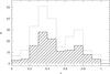 |
Fig. 1 Redshift distribution of all galaxies in our survey (solid line, 238 galaxies; one fill-up target at z = 1.49 is omitted in this plot) and our kinematic sample, that is, all galaxies used in our kinematic analysis (hashed histogram, 124 galaxies). The selection criterion for the latter subsample is detailed in Sect. 4.3. |
4.1. Absolute magnitudes
We opted to construct the B-band Tully-Fisher relation in this study to be sensitive for recent or ongoing star formation. A great advantage for this is the multiband imaging at hand that closely matches the rest-frame B-band for any galaxy redshift in our sample. To determine the B-band luminosities MB, we used the observed filter Xobs that best matched the rest-frame B-band to derive the k-correction through synthetic photometry and computed the transformation Xobs → Brest. In the FDF, we used the transformation Bobs → Brest at redshifts z< 0.25, gobs → Brest at 0.25 <z< 0.55, Robs → Brest at 0.55 <z< 0.85 and Iobs → Brest at z> 0.85. For the galaxies stemming from the WHDF, we used Bobs → Brest at z< 0.3, Robs → Brest at 0.3 <z< 0.7 and Iobs → Brest at z> 0.7. Thanks to this approach, the k-correction only weakly depends on the spectral energy distribution of a given galaxy: if the spectral classification were incorrect by ΔT = 2 (which corresponds to the spectrum of an Sa galaxy mistakenly classified as type Sb, for example), the resulting systematic k-correction error would be σk< 0.1 mag across the whole redshift range covered by our data.
We corrected for intrinsic absorption AB that is due to the dust disk following the approach by Tully et al. (1998). This formalism is inclination- and Vmax-dependent: disks that are observed more edge-on have a higher extinction than more face-on ones, and more massive disks, that is, galaxies with higher Vmax, have a higher extinction than less massive ones.
To summarize, the absolute B-band magnitudes were computed as  (1)where mX is the total apparent brightness in filter X,
  is the Galactic absorption for filter X, corrected using the maps by Schlegel et al. (1998), DM is the distance modulus, kB is the k-correction, and AB is the correction for intrinsic dust absorption in rest-frame B.
4.2. Structural parameters
We derived the structural parameters of the galaxies such as disk inclination, disk scale length rd, and bulge-to-total ratio B/T on the HST/ACS images using the GALFIT package by Peng et al. (2002). It allows simultaneous fitting of multiple two-dimensional surface brightness profiles to the galaxy under scrutiny and to neighboring objects (the importance of these simultaneous fits is discussed for instance in Häußler et al. 2007). GALFIT requires an input point spread function (PSF) for the convolution of the model profiles. We constructed PSFs for the FDF and WHDF separately from ~20 unsaturated stars in each field. Both have a FWHM of 0.12 arcsec, corresponding to a spatial resolution of ~0.7 kpc at z = 0.5.
The surface brightness profiles of all galaxies in our sample were fitted with two different setups: i) a single Sérsic profile with free index nser or ii) a two-component model with an exponential profile for the disk and a Sérsic profile with fixed index nser = 4 for the bulge. The best-fit parameters from method i) were used as initial guess values for method ii).
All fit residuals were visually inspected, and in a few cases, constraints on parameters such as the bulge effective radius were necessary to avoid a local χ2 minimum in the fitting process. For our analysis, we mostly used the disk parameters from the bulge or disk decomposition, that is, method ii). Only in a few cases where the two-component fit of an evidently bulgeless disk did not converge did we keep the parameters from the single Sérsic fit. We stress that for the analysis presented here, the most important parameters are the inclination i, position angle θ, and scale length rd of the disk. These showed only small differences between the two fitting methods. This is mainly because the vast majority of the FDF/WHDF disks have only small bulges or even no detectable bulge at all; the median bulge-to-total ratio is ⟨ B/T ⟩ = 0.06.
GALFIT only returns random errors on the best-fit parameters. These are very small (<1 %) throughout our sample. To gain a more realistic estimate of the systematic errors on rd, we relied on our own previous analysis of HST/ACS images using GALFIT in Böhm et al. (2013). In that work, we investigated the effect of an active galactic nucleus on the morphologies of host galaxies at redshifts 0.5 <z< 1.1 as quantified with GALFIT. For a negligible central point source, we found a typical systematic error of 20 % on galaxy sizes (see Fig. 7d in Böhm et al. 2013). This value hence represents the systematic size error for galaxies with the light profiles of pure disks or disks with only weak bulges; this is the case for the vast majority of galaxies in our sample. We therefore adopt this error on rd in the following.
It is well-known that the observed disk scale length depends on the wavelength regime (see, e.g., de Jong 1996), in the sense that rd is smaller in redder filters. The effect is very weak in the F814W filter for the redshifts covered by our sample and at maximum corresponds to an overestimate of rd by 11% for the highest redshift galaxy in our sample, at z = 0.97. We corrected (i.e., reduced) all measured disk scale lengths for this effect depending on a given galaxy’s redshift to make them directly comparable.
4.3. Kinematics
Rotation curves (rotation velocity as a function of radius) were extracted from the two-dimensional spectra by fitting Gaussian profiles to the emission lines stepwise along the spatial axis. We used a boxcar of three pixels, averaging over a given spectral row and its two adjacent rows. This approach increases the signal-to-noise ratio (S/N) without loss in spatial resolution. The boxcar size corresponds to 0.6 arcsec in the FDF spectra and 0.75 arcsec in the WHDF spectra; both values are below the average seeing during spectroscopy. All detected emission lines were used, and the rotation curve with the best S/N and largest spatial extent was used as reference in the further analysis. The typical error on the rotation velocity at a given galactocentric radius is 10−20 km s-1. Approximately half of the reference rotation curves stem from the [O II] doublet, the other half is based on the [O III], Hβ, or Hα line. The vast majority of the rotation curves extracted from different emission lines agreed within the errors of the Gaussian fits in the sense that the rotation velocities at given radius agreed within their errors.
The derivation of the maximum rotation velocity Vmax of distant galaxies is a challenging task. At z ≈ 0.5, the half-light radius of a Milky Way-type galaxy is similar to the slit width and the typical seeing FWHM. This leads to strong blurring effects in the observed rotation curves. It is mandatory to take these effects into account to avoid underestimates of Vmax. To tackle this problem, we introduced a method that simulates all steps of the observation process, from the intrinsic two-dimensional rotation velocity field to the extracted one-dimensional rotation curve.
The intrinsic rotation velocity field, which is unaffected by any geometrical, atmospherical, or instrumental effects, is generated assuming a linear rise of the rotation velocity Vrot(r) at radii r<rt, where rt is the so-called turnover radius, and a convergence of Vrot(r) to a constant value Vmax at r>rt (Courteau 1997). We adopted a turnover radius equal to the scale length rd,gas of the emitting ionized gas disk; rd,gas, in turn, was computed from the stellar disk scale length rd following Ryder & Dopita (1994). The intrinsic velocity field was then transformed into a simulated rotation curve including the following effects:
-
1.
disk inclination angle i;
-
2.
misalignment angle δ between the slit orientation and the apparent major axis;
-
3.
seeing during spectroscopy;
-
4.
luminosity profile weighting perpendicular to the slit direction;
-
5.
blurring effect due to the slit width in direction of dispersion; this is the optical equivalent to beam smearing in radio observations.
The simulated rotation curve was then fit to the observed one to infer the intrinsic maximum rotation velocity Vmax.
We here used Vmax as the only free parameter in the rotation curve fitting process. The other parameters were held fixed based on the observed disk inclination, position angle, scale length, etc. For testing purposes, we used rt as a second fitting parameter and found that the results on Vmax agreed with the single-parameter fits within the errors for ~90% of the objects. This is probably due to the strong blurring effects that limit or even erase information on the rotation curve shape at small galactocentric radii.
We also investigated whether our results depend on the intrinsic topology of Vrot(r). When we used the more complex universal rotation curve (URC) shape introduced by Persic et al. (1996) instead of the parametrization by Courteau et al. (1997), the recomputed Vmax values agree with the Courteau-based ones for 96% of our sample. In brief, the URC was inferred from >1000 observed rotation curves of local spiral galaxies; it comprises a mass-dependent velocity gradient. Very low-mass spirals show an increasing rotation velocity even at large radii, whereas the rotation curves of very high-mass spirals moderately decline in that regime. Our results on Vmax are not sensitive to the choice of the intrinsic rotation curve shape for two reasons. First, our sample mainly covers intermediate masses, where the URC does not introduce a velocity gradient at large galactocentric radii. Second, the radial extent of the observed rotation curves, typically four disk scale lengths , might be too small to reliably detect a potential velocity gradient in the outer disk.
To ensure a correct analysis of the scaling relations, we visually inspected all rotation curves to identify those that a) showed kinematic perturbations or b) had an insufficient spatial extent and did not probe the regime where Vrot(r) converges to Vmax; in extreme cases, these curves show solid-body rotation. During this visual inspection, we rejected 101 objects from the data set of 238 galaxies with determined redshifts, corresponding to a fraction of 42%. Another 13 galaxies were not considered for further analysis because the rotation curve fitting yielded a very large error on Vmax, with a relative error σvrel = σvmax/Vmax> 0.5 (errors on Vmax stem from fitting the synthetic rotation curves to the observed rotation curves through χ2 minimization). The excluded 13 galaxies are relatively faint (median total apparent R-band brightness ⟨ R ⟩ = 22.42, compared to ⟨ R ⟩ = 21.81 for the rest of the sample with derived Vmax) and their rotation curves show slight asymmetries; otherwise these galaxies have properties similar to the remaining sample.
The 124 galaxies with a reliable Vmax constitute our kinematic sample. It covers a range 25 km s-1<Vmax< 450 km s-1 with a median value of ⟨ Vmax ⟩ = 145 km s-1. The median of the relative error of the maximum rotation velocities is ⟨ σvrel ⟩ = 0.19. This error in general is larger toward lower values of Vmax, in other words, toward low-mass galaxies, and smaller towards higher values of Vmax, or toward high-mass galaxies. Table 1 lists the main parameters of ten galaxies as an example (the full table comprising 124 galaxies is available at the CDS): object ID, redshift, maximum rotation velocity, B-band absolute magnitude, and disk scale length.
Main galaxy parameters.
4.4. Tully-Fisher relation
We show the distribution of our kinematic sample in rotation velocity − luminosity space in Fig. 2. Our data representing a median redshift of z = 0.45 are shown as solid symbols in comparison to the local Tully-Fisher relation as given by Tully et al. (1998):  (2)which is shown as a dashed line in Fig. 2; the dotted lines indicate the 3σ scatter of the local data. Local and distant galaxies are consistently corrected for intrinsic dust absorption following the approach of Tully et al. (1998). The redshift distribution of our kinematic sample of 124 galaxies is shown in Fig. 1. It is very similar to the full sample of 238 galaxies with determined redshifts. The majority of the distant galaxies are located within the 3σ limits of the local TFR (see Fig. 2). Interestingly, almost all galaxies with rotation velocities log Vmax< 2 fall on the high-luminosity side of the local relation, and the eight galaxies with log Vmax< 1.8 are even located above the 3σ limits of the local TFR. Three possible explanations have to be considered.
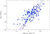 |
Fig. 2 Rest-frame B-band Tully-Fisher diagram, showing a comparison between our sample of 124 disk galaxies at a median redshift ⟨ z ⟩ ≈ 0.5 (solid symbols) and the local Tully-Fisher relation as given by Tully et al. (1998; the black dashed line indicates the fit to the local data (not shown in this figure); the dotted lines give the local 3σ scatter). The blue solid line shows the fit to the distant sample (with the slope fixed to the local value), which is offset from the local Tully-Fisher relation toward higher luminosities by ⟨ ΔMB ⟩ = −0.47 ± 0.16 mag. |
First, Vmax might be underestimated for low-mass disk galaxies: optical rotation curves of low-mass disks in the local Universe often have a positive rotation velocity gradient even at the largest covered radii (e.g., Persic et al. 1996). As outlined in Sect. 4.3, we did not find significant changes in Vmax when adopting intrinsic rotation velocity fields with positive gradients in low-mass galaxies (using the prescriptions presented in Persic et al.). However, the spatial extent of the rotation curves in our sample (as well as other samples at similar redshifts) is typically three to four times the optical disk scale length, which might be insufficient to constrain potential Vrot gradients.
Second, the observations might indicate a mass-dependent evolution in luminosity that is larger for low-mass disk galaxies than for high-mass ones. This might be interpreted as a manifestation of the down-sizing phenomenon (e.g., Kodama et al. 2004). A third interpretation would be that the apparent mass-dependency is only mimicked by the effect of the magnitude limit of our sample. It has been demonstrated by numerous authors (e.g., Willick 1994) that toward lower Vmax, mainly galaxies on the high-luminosity side of a parent unbiased Tully-Fisher distribution enter an observed sample. For a detailed discussion of this magnitude limit effect, see Appendix A.
While the first interpretation outlined above is purely kinematical, the other two only concern the luminosity, either in the rank of a physical effect (down-sizing) or a selection effect (magnitude bias). Because our targets have been selected for observation using a limit in apparent magnitude, which is a common and well-motivated approach, the third scenario seems much more likely than the second. We again refer to Appendix A for a more detailed discussion of this topic. Toward higher Vmax, however, most rotation curves should be flat even beyond the radii probed by our data, provided that the internal mass distribution in intermediate-z and local disk galaxies is similar (e.g., Sofue & Rubin 2001). Furthermore, the effect of the magnitude limit becomes negligible toward higher Vmax (e.g., Giovanelli et al. 1997).
We note that overestimated luminosities at low Vmax are highly unlikely because the ground-based photometry is very deep and we computed MB from the filter which best matches the B-band in rest-frame, which ensures very small total errors on the absolute magnitudes (the combined random and systematic errors are σMB< 0.12 mag for all galaxies). The offsets of the slow rotators from the local TFR cannot be attributed to an evolution in redshift either: the median redshift of these galaxies (⟨ z ⟩ = 0.37 for the eight TFR outliers at log Vmax< 1.8) is lower than that of the remaining sample (⟨ z ⟩ = 0.45). We revisit the question of any redshift dependencies below.
Computing the offsets of individual galaxies from the local TFR (as given in Eq. (2)) through  (3)we find that the distant galaxies are more luminous for a given Vmax than their local counterparts, with a median value ⟨ ΔMB ⟩ = −0.47 ± 0.16 mag (shown as a solid line in Fig. 2). The scatter in ΔMB, that is, the scatter of the distant TFR under the assumption of the local slope, is σobs = 1.28 mag, which is 2.3 × σobs of the local B-band TFR, for which Tully et al. give σobs = 0.55 mag. The fixed-slope fit to the distant data shows a significant overluminosity of the distant disk galaxies. However, the scatter of the distant sample is large, more than twice the local value, and the vast majority of the distant galaxies are located within the 3σ limits of the local TFR. This large scatter might in part be due to the broad range in redshifts (see Fig. 1), as the evolution in luminosity might depend on look-back time (other possible sources of increased scatter are discussed in Sect. 5). We therefore now shift our focus from the global evolution in luminosity to the evolution of individual galaxies.
We show the offsets from the local TFR, computed following Eq. (3), as a function of redshift in Fig. 3. The errors on ΔMB are computed through error propagation from the errors on Vmax and MB. The TFR offsets ΔMB show an evolution toward higher luminosities at higher redshifts. This is confirmed by a linear fit to the full sample, which yields  (4)At given Vmax, disk galaxies at z = 1 are on average more luminous by ΔMB = −1.2 ± 0.5 mag according to this fit. As shown in Fig. 3, the fit to our data agrees with Dutton et al. (2011), who used combined N-body simulations and semi-analytical models. With N-body and hydrodynamical simulations, Portinari & Sommer-Larsen (2007) found ΔMB = −0.85 mag at z = 1, which excellently agrees with the Dutton et al. value of ΔMB = −0.9 mag and our own result. The nonlinear evolution of the model prediction (see Fig. 3) cannot be confirmed with our data, however. A second-order polynomial fit agrees with the linear fit to within ± 0.1 mag throughout the probed redshift range.
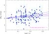 |
Fig. 3 Offsets ΔMB of the galaxies in our sample from the local Tully-Fisher relation, displayed as a function of redshift. The galaxies show increasing overluminosities toward longer look-back times, reaching ΔMB = −(1.2 ± 0.5) mag at z = 1 according to a linear fit, depicted as a blue solid line and dashed lines indicating the 1σ error range. The observed luminosity evolution agrees well with predictions from numerical simulations by Dutton et al. (2011; solid magenta line), who found ΔMB = −0.9 at redshift unity. The dotted line illustrates no evolution in luminosity. |
4.5. Velocity-size relation
We now investigate the rotation velocity-size relation. For this purpose, we use the data on ~1100 local disk galaxies by Haynes et al. (1999b). Since the electronically available disk sizes are given as isophotal diameters at 23.5 mag I-band surface brightness, we transformed these into disk scale lengths assuming an average central surface brightness of μI = 19.4 mag, as given in Haynes et al. (1999a).
With a bisector fit to the local data, that is, with a combination of two least-squares fits with the dependent and independent variables interchanged (e.g., Isobe 1990), we find  (5)Figure 4 shows our data compared to the local VSR as defined by Eq. (5). A few galaxies at the lowest Vmax are scattered toward large radii in VSR space. These are galaxies that also lie above the 3σ-limits of the local TFR. Either Vmax is underestimated for these galaxies, or they are more luminous and larger than expected for their maximum rotation velocities.
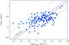 |
Fig. 4 Velocity-size relation (VSR): disk scale length rd as a function of maximum rotation velocity Vmax. We show a comparison between our ⟨ z ⟩ ≈ 0.5 data (circles) and the local VSR as found with data from Haynes et al. (1999b; the black dashed line indicates the fit to the local data (not shown in this figure) and the dotted lines depict the 3σ scatter). The blue solid line shows the fit to the distant sample, which is offset to smaller disk sizes by ⟨ Δlog rd ⟩ = −0.10 ± 0.05 dex. |
We computed the offsets from the local VSR as  (6)which yields a median of ⟨ Δlog rd ⟩ = −0.10 ± 0.05 (displayed as a solid line in Fig. 4). The scatter in the distant sample is σobs = 0.27 dex, which is 2.1 times larger than the local value of σobs = 0.13 dex.
We now again focus on a potential evolution with look-back time. Figure 5 shows the VSR offsets as a function of redshift. Errors on Δlog rd are propagated from errors on Vmax and rd. Using a linear fit, we find  (7)Disk galaxies at z = 1 were therefore smaller than local disks by a factor of
  on average, for a given Vmax. This reflects ongoing disk growth with cosmic time, as expected for hierarchical structure formation (e.g., Mao et al. 1998). As a test, we also applied a second-order polynomial fit to the VSR offsets, not finding a significant second-order term and large errors. Similar to the TFR offsets, we therefore cannot reproduce the nonlinear evolution with cosmic time predicted by the Dutton et al. (2011) models.
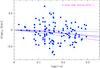 |
Fig. 5 Offsets Δlog rd of our galaxy sample from the local velocity-size relation (see Fig. 4) as a function of redshift. Negative values in Δlog rd correspond to smaller sizes at given maximum rotation velocity Vmax. We find successively smaller disks toward higher redshifts. A linear fit to our data (displayed as a blue solid line, and dashed lines indicate the 1σ error range) shows that disk galaxies at z = 1 were smaller than their local counterparts by a factor of ~1.5. For comparison, the solid magenta line shows predictions from simulations by Dutton et al. (2011). The dotted line illustrates no evolution in size. |
5. Discussion
To interpret the observed evolution of our disk galaxy sample in Tully-Fisher space, we need to recall that several processes might occur between previous cosmic epochs and the local Universe, and it might be a combination of these processes that governs the evolution in ΔMB. For the following discussion, we recall that the maximum rotation velocity Vmax is a proxy for the total (virial) mass of a disk galaxy such that  (e.g., van den Bosch 2002). Since the virial mass is dominated by dark matter, and the optical luminosity is dominated by stellar light, the optical TFR reflects a fundamental interplay between dark and baryonic matter.
The stellar populations of distant galaxies probably have a younger mean age; this translates into a lower stellar M/L ratio and, in turn, a lower total (baryonic and dark matter) M/L ratio than the local ratio. At given Vmax, distant galaxies therefore would be expected to be more luminous than local ones, particularly in the B-band considered here, which is sensitive to high-mass stars with short lifetimes. The gas mass fractions are probably higher toward higher redshifts (e.g., Puech et al. 2010), corresponding to higher total M/L ratios and TFR offsets ΔMB> 0. Furthermore, as less gas has been converted into stars, stellar masses M∗ might be lower at given Vmax, and this, in turn, would lead to lower luminosities and, again, positive TFR offsets. The observational census on the evolution in stellar mass is somewhat unclear at z< 1: for example, Puech et al. (2008) found a decrease in stellar mass of  dex up to z = 0.6, while Miller et al. (2011) reported a small and statistically insignificant evolution of ΔM∗ = −0.04 ± 0.07 dex up to z = 1. Using simulations, Dutton et al. (2011) predicted a growth in stellar mass by ~0.15 dex between z = 1 and z = 0 at fixed Vmax.
We do not imply that for an individual galaxy the evolutionary path in TFR space would at all times be purely in luminosity between z = 1 and z = 0. If a disk galaxy would undergo a minor merger, for example, then the remnant would, after relaxation of the kinematical disturbances, most likely be located at a higher Vmax and have a higher luminosity than before the encounter. During or shortly after the minor merger, such a galaxy would not enter our kinematic sample even if it were covered by our observations because it would feature a disturbed rotation curve. This is just to give an example that we do not claim disk galaxy evolution at z< 1 to solely proceed parallel to the luminosity axis in TFR space. A minor merger with a low-mass satellite would probably lead to an increase of the total M/L ratio because dwarf galaxies have higher dark matter mass fractions than galaxies in the M∗ regime (e.g., Moster et al. 2010). Lacking data on gas mass fractions, we cannot infer dark matter mass fractions for our sample. For the ratio M∗/Mvir between stellar mass and virial mass, Conselice et al. (2005) observationally found a mild decrease between z ≈ 1 and z ≈ 0, corresponding to a slight increase in total M/L ratio. Using semi-analytic models, Mitchel et al. (2016) inferred a basically constant M∗/Mhalo at 0 <z< 1 (cf. their Fig. 2).
Based on the processes described above, the younger stellar populations toward higher redshifts, potentially in combination with slightly lower dark matter mass fractions, most likely dominate in our sample because we find an increase in luminosity of ΔMB = −1.2 ± 0.5 at given Vmax toward z = 1, hence a decrease in total M/L ratio. Our result agrees with previous observational findings by Bamford et al. (2006) or Miller et al. (2011), for example, and also with predictions from simulations by Portinari & Sommer-Larsen (2007) and Dutton et al. (2011). A stellar population modeling of 108 galaxies from our sample (Ferreras et al. 2014) revealed the well-known downsizing effect: the distant high-mass disk galaxies began forming their stars at higher redshifts and on shorter timescales than the low-mass disks.
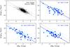 |
Fig. 6 Combined look at the offsets ΔMB from the Tully-Fisher relation and the offsets Δlog rd from the velocity-size relation. Top left: local sample from Haynes et al. (1999b; no error bars shown for clarity), showing a correlation between the two parameters (the dashed and dotted lines show the fit and 3σ scatter). Top right, bottom left and bottom right: distribution of our data in three redshift bins comprising 41−42 galaxies each, with a fixed-slope fit indicated by a solid line. The local fit and 3σ scatter are displayed for comparison in each panel. These figures show the combined evolution in luminosity and size toward higher redshifts. See text for details. |
The observed evolution in disk scale length (Fig. 5) reflects the growth of disks with ongoing cosmic time. This evolution is expected in an LCDM cosmology with hierarchical structure growth. Based on theoretical considerations, this has been predicted by Mao et al. (1998). In the cosmology adopted here, the computations by these authors correspond to a disk size increase by a factor of ~1.9 between z = 1 and z = 0 at given Vmax; larger than what we find, but almost in agreement within the errors. The fit to the observed evolution given in Eq. (7) corresponds to Δlog rd = −0.16 dex at z = 1. This is a slightly stronger evolution in size than given in the observational study of Vergani et al. (2012; these authors derived Δlog rd = −0.12 dex at z = 1.2), and a slightly weaker evolution than predicted with semi-analytical models by Dutton et al. (2011), who find Δlog rd = −0.19 dex at z = 1. Candidate processes to explain the disk growth toward z = 0 are accretion of cold gas or minor mergers with small satellites. Any major mergers in the cosmic past of galaxies in our kinematical sample must have occurred several Gyr ago so that the merger remnant could regrow a rotationally supported disk (e.g., Governato et al. 2009). Major merger remnants are kinematically cold only in special pre-merger configurations (e.g., Springel & Hernquist 2005).
We note that the Haynes et al. (1999b) sample that we used as a local VSR reference comprises disk scale lengths derived in the I-band, the response function of which is very similar to that of the F814W filter used for our HST imaging. Since we corrected all scale lengths to rest-frame in our data set, local reference and distant galaxies can be directly compared. If the required correction for the wavelength dependence of rd (following de Jong 1996) were omitted, our sample would yield a weaker size evolution, corresponding to Δlog rd = −0.11 dex at z = 1 for a given Vmax.
Our analysis so far has shown that the disk galaxy population as a whole evolves in luminosity and size over the redshifts covered by our data. However, we do not know yet how this combined evolution proceeds for individual galaxies. Do the galaxies with the strongest evolution in size also show the strongest evolution in luminosity, or is the picture more complex?
To study this in more detail, we compare the offsets from the Tully-Fisher relation ΔMB to the offsets from the velocity-size relation Δlog rd as shown in Fig. 6. We first consider the situation in the present-day universe: the upper left panel shows the local sample from Haynes et al. (1999b). The offsets ΔMB of these galaxies are computed from the local TFR as derived with the same sample, and the offsets Δlog rd from the local VSR (as given in Eq. (5)) are also based on the same sample. By construction, the median of both parameters is zero. At first glance, it might be surprising that ΔMB and Δlog rd are correlated: the dashed line depicts a fit to the local data; the dotted lines illustrate threetimes the local scatter, which in terms of Δlog rd is σ = 0.09 dex. This correlation can be understood as a result of the fact that disk galaxies populate a planein the three-dimensional parameter space span by maximum rotation velocity, luminosity, and size (e.g., Koda et al. 2000). Since the TFR is a projection of this fundamental plane, any deviation of a galaxy in the local Universe from the TFR depends partly on its size, or, more precisely, on its position in luminosity-size space. In other words, Fig. 6 is equivalent to an edge-on view on the fundamental plane of disk galaxies in the direction of, but not parallel to, the Vmax axis.
We divided our sample into three redshift bins z< 0.36, 0.36 <z< 0.59 and z> 0.59, each holding 41−42 galaxies. These subsamples are shown in the other panels of Fig. 6 in comparison to the local fit and scatter. For the distant data, TFR offsets ΔMB and VSR offsets Δlog rd were computed as described in Sects. 4.4 and 4.5. To interpret these graphs, it has to be kept in mind that any evolution in luminosity and/or size is imprinted on the correlation between ΔMB and Δlog rd explained above.
We find that toward higher redshifts, the distant galaxies gradually shift away from the local ΔMB–Δlog rd relation. Using fixed-slope fits to determine the offsets from the local relation in terms of Δlog rd, we infer an evolution of −0.08 ± 0.06 dex, −0.19 ± 0.08 dex, and −0.29 ± 0.07 dex at redshifts z< 0.36, 0.36 <z< 0.59, and z> 0.59, respectively. These offsets are depicted by solid lines in each of the distant data panels of Fig. 6. These deviations from the local relation are larger than the evolution in size alone (see Sect. 4.5), since here Δlog rd is a combination of the evolution in size and (in projection) luminosity. The scatter in the distant ΔMB–Δlog rd relation is larger than the local scatter: our data yield 0.22 dex at z< 0.36, 0.18 dex at 0.36 <z< 0.59, and 0.20 dex at z> 0.59. Similar to the situation in TFR and VSR space, the scatter in the distant data hence is approximately doubled compared to the local reference, which shows σ = 0.09 dex.
The fact that the correlation between ΔMB and Δlog rd holds up to redshifts z ≈ 1 has consequences for the combined evolution in luminosity and size of individual galaxies. This becomes particularly clear in the z > 0.59 bin, which represents the longest look-back times (5.6 Gyr <tlookback < 7.7 Gyr) and is most sensitive to the evolution with cosmic time. The shape of the distribution does not appear to be changed with respect to the local Universe, but merely shifted toward higher luminosities and smaller sizes. The galaxies that evolved strongest in luminosity are not those that evolved strongest in size, and vice versa. The galaxies with the strongest decrease in size scatter around ΔMB ≈ 0, and the galaxies with the strongest evolution in luminosity mostly show Δlog rd > 0 and hence are larger than their local counterparts at the same Vmax.
We finally address the scatter of the intermediate-redshift scaling relations. The observed scatter at z ≈ 0.5 (σobs = 1.28 mag and σobs = 0.27 dex for the TFR and VSR, respectively) is approximately doubled with respect to the local reference data. The TFR scatter we find is smaller than in the sample of Weiner et al. (2006, σobs ≈ 1.5 mag), similar to Fernàndez Lorenzo et al. (2010, σobs ≈ 1.2 mag), and slightly larger than the value given by Bamford et al. (2006, σobs ≈ 1.0 mag); these are all studies at redshifts similar to our data. Part of the observed distant scatter stems from the uncertainties of the Vmax derivation and the observational limitations, such as beam smearing and limited spatial resolution. We now clarify whether the increased scatter is driven by the measurement errors of the galaxy parameters or is due to an increase of the intrinsic scatter. The observed scatter σobs of the TFR comprises contributions from the errors σmb on the absolute magnitudes, errors σvmax on the maximum rotation velocities and the intrinsic scatter σint such that  (8)where c is the TFR slope. Our kinematic sample of 124 galaxies yields an intrinsic scatter σint ≈ 1.1 mag. In comparison to other studies at similar redshifts, our result is only slightly higher than the value given by Bamford et al. (2006, σint ≈ 0.9 mag), but much higher than the σint ≈ 0.7 mag derived by Miller et al. (2011). Tully et al. (1998) did not give the intrinsic scatter for their local TFR sample, but the observed B-band scatter σobs = 0.55 mag suggests that the intrinsic scatter is on the order σint ≈ 0.3−0.4 mag. Our analysis and those of Bamford et al. and Miller et al. hence show an increased intrinsic TFR scatter at intermediate redshifts. This increase might be due to a larger contribution of non-circular motions, for example, that is, to kinematically heated disks (e.g., Förster-Schreiber et al. 2009) or more frequent mismatches between photometric and kinematic position angle (e.g., Kutdemir et al. 2010) than locally.
In principle, it would also be possible that the stellar populations have an effect on the intrinsic TFR scatter, for example due to a broader distribution in stellar M/L ratios toward higher redshifts. To investigate this, we computed the stellar B-band M/L ratios from the absorption-corrected rest-frame (B−R) colors following Bell & de Jong (2001) for all galaxies in our sample. We defined three redshift bins, using only the 47 galaxies with stellar masses M∗> 1010M⊙ (which we detect up to redshift z ≈ 1) to minimize the effect of the correlation between stellar M/L ratio and galaxy stellar mass. The three resulting redshift bins with 15−16 galaxies each have median redshifts of ⟨ z ⟩ = 0.36, ⟨ z ⟩ = 0.63, and ⟨ z ⟩ = 0.84. We found an rms of the B-band stellar mass-to-light ratio of σM/L = 0.98 [ (M/LB)⊙ ] in the lowest redshift bin, σM/L = 0.46 [ (M/LB)⊙ ] at ⟨ z ⟩ = 0.63, and σM/L = 0.88 [ (M/LB)⊙ ] at ⟨ z ⟩ = 0.84. At least as far as stellar mass-to-light ratios are concerned, we therefore find no indication that the evolution in the intrinsic TFR scatter might be (partly) driven by the stellar populations.
6. Conclusions
Using the FORS instruments of the ESO Very Large Telescope, we have constructed a sample of 124 disk galaxies up to redshift z ≈ 1 with determined maximum rotation velocity Vmax. Structural parameters such as disk inclination and scale length were derived on HST/ACS images. We analyzed the distant Vmax− luminosity (Tully-Fisher) and Vmax− size relations and compared them to reference samples in the local universe. Our main findings can be summarized as follows:
-
1.
At given Vmax, disk galaxies are more luminous (in rest-frame B-band) and smaller (in rest-frame I-band) toward higher redshifts. By z = 1, we found a brightening of ΔMB ≈ −1.2 mag in absolute B-band magnitude and a decrease in size by a factor of ~1.5.
-
2.
The scatter in the Tully-Fisher and VSRs at z ≈ 0.5 is increased by a factor of approximately two with respect to the local Universe.
-
3.
The observed evolution in luminosity and size over the past ~8 Gyr agrees well with predictions from numerical simulations (e.g., Portinari & Sommer-Larsen 2007; Dutton et al. 2011).
-
4.
An analysis of the combined evolution in luminosity and size revealed that the galaxies that show the strongest evolution toward smaller sizes at z ≈ 1 are not those that feature the strongest evolution in luminosity, and vice versa. The galaxies with the strongest deviations from the local VSR toward smaller disks have luminosities compatible with the local TFR, while the galaxies with the strongest evolution in luminosity are slightly larger than their local counterparts at similar Vmax.
In the next paper of this series, we will conduct a comparison between the kinematics of distant disk galaxies observed with two-dimensional (slit) and three-dimensional (integral field unit) spectroscopy, in particular with respect to scaling relations like the TFR and VSR (Böhm et al., in prep.). Another paper will focus on the evolution of the correlation between the maximum rotation velocity of the disk and the stellar velocity dispersion in the bulge (Böhm et al., in prep.).
Acknowledgments
We thank the anonymous referee for a detailed report that was very helpful in improving the manuscript. A.B. is grateful to the Austrian Science Fund (FWF) for funding (projects P19300-N16 and P23946-N16). The authors thank B. Bösch (Innsbruck) for providing a Python code of the Kelson (2003) method for improved sky subtraction in the FORS2/MXU spectra. This publication is supported by the Austrian Science Fund (FWF).
References
- Bamford, S. P., Aragon-Salamanca, A., & Milvang-Jensen, B. 2006, MNRAS, 366, 308 [NASA ADS] [CrossRef] [Google Scholar]
- Bender, R., Appenzeller, I., Böhm, A., et al. 2001, in Deep Fields, eds. S. Cristiani, A. Renzini, & R. E. Williams, ESO Astrophys. Symp. (Springer), 96 [Google Scholar]
- Burstein, D., Bender, R., Faber, S. M., & Nolthenius, R. 1997, AJ, 114, 1365 [NASA ADS] [CrossRef] [Google Scholar]
- Bell, E. F., & de Jong, R. S. 2001, ApJ, 550, 212 [NASA ADS] [CrossRef] [Google Scholar]
- Böhm, A., & Ziegler, B.L. 2007, ApJ, 668, 846 [NASA ADS] [CrossRef] [Google Scholar]
- Böhm, A., Ziegler, B. L., Saglia, R. P., et al. 2004, A&A, 420, 97 [NASA ADS] [CrossRef] [EDP Sciences] [Google Scholar]
- Böhm, A., Wisotzki, L., Bell, E. F., et al. 2013, A&A, 549, A46 [NASA ADS] [CrossRef] [EDP Sciences] [Google Scholar]
- Bösch, B., Böhm, A., Wolf, C., et al. 2013a, A&A, 549, A142 [NASA ADS] [CrossRef] [EDP Sciences] [Google Scholar]
- Bösch, B., Böhm, A., Wolf, C., et al. 2013b, A&A, 554, A97 [NASA ADS] [CrossRef] [EDP Sciences] [Google Scholar]
- Conselice, C. J., Bundy, K. E., Richard, S., et al. 2005, ApJ, 628, 160 [NASA ADS] [CrossRef] [Google Scholar]
- Courteau, S. 1997, AJ, 114, 2402 [NASA ADS] [CrossRef] [Google Scholar]
- Cresci, G, Hicks, E. K. S., Genzel, R., et al. 2009, ApJ, 697, 115 [NASA ADS] [CrossRef] [Google Scholar]
- de Jong, R. S. 1996, A&A, 313, 377 [NASA ADS] [Google Scholar]
- Dressler, A., Lynden-Bell, D., Burstein, D., et al. 1987, ApJ, 313, 42 [NASA ADS] [CrossRef] [Google Scholar]
- Dutton, A. A., van den Bosch, F. C., Faber, S. M., et al. 2011, MNRAS, 410, 1660 [NASA ADS] [Google Scholar]
- Epinat, B., Contini, T., Le Fèvre, O., et al. 2009, A&A, 504, 789 [NASA ADS] [CrossRef] [EDP Sciences] [Google Scholar]
- Fernàndez Lorenzo, M., Cepa, J., Bongiovanni, A., et al. 2010, A&A, 521, A27 [NASA ADS] [CrossRef] [EDP Sciences] [Google Scholar]
- Ferreras, I., Böhm, A., Ziegler, B. L., & Silk, J. 2014, MNRAS, 437, 1872 [NASA ADS] [CrossRef] [Google Scholar]
- Flores, H., Hammer, F., Puech, M., Amram, P., & Balkowski, C. 2006, A&A, 455, 107 [NASA ADS] [CrossRef] [EDP Sciences] [Google Scholar]
- Förster-Schreiber, N., Genzel, R., Bouché, N., et al. 2009, ApJ, 706, 1364 [NASA ADS] [CrossRef] [Google Scholar]
- Giovanelli, R., Haynes, M. P., Herter, T., & Vogt, N. P. 1997, AJ, 113, 53 [NASA ADS] [CrossRef] [Google Scholar]
- Gnerucci, A., Marconi, A., Cresci, G., et al. 2011, A&A, 528, A88 [NASA ADS] [CrossRef] [EDP Sciences] [Google Scholar]
- Governato, F., Willman, B., Mayer, L., et al. 2007, MNRAS, 374, 1479 [NASA ADS] [CrossRef] [Google Scholar]
- Governato, F., Brook, C. B., Brooks, A. M., et al. 2009, MNRAS, 398, 312 [NASA ADS] [CrossRef] [Google Scholar]
- Häußler, B., McIntosh, D. H., Barden, M., et al. 2007, ApJS, 172, 615 [NASA ADS] [CrossRef] [EDP Sciences] [Google Scholar]
- Haynes, M. P., Giovanelli, R., Salzer, J. J., et al. 1999a, AJ, 177, 1668 [NASA ADS] [CrossRef] [Google Scholar]
- Haynes, M. P., Giovanelli, R., Salzer, J. J., et al. 1999b, AJ, 177, 2039 [NASA ADS] [CrossRef] [Google Scholar]
- Heidt, J., Appenzeller, I., Gabasch, A., et al. 2003, A&A, 398, 49 [NASA ADS] [CrossRef] [EDP Sciences] [Google Scholar]
- Isobe, T., Feigelson, E. D., Akritas, M. G., & Babu, G. J. 1990, ApJ, 364, 104 [NASA ADS] [CrossRef] [EDP Sciences] [Google Scholar]
- Jaffé, Y. L., Aragón-Salamanca, A., Kuntschner, H., et al. 2011, MNRAS, 417, 1996 [NASA ADS] [CrossRef] [Google Scholar]
- Kassin, S. A., Weiner, B. J., Faber, S. M., et al. 2007, ApJ, 660, L35 [NASA ADS] [CrossRef] [Google Scholar]
- Kelson, D. D. 2003, PASP, 155, 688 [NASA ADS] [CrossRef] [Google Scholar]
- Koda, J., Sofue, Y., & Wada, K. 2000, ApJ, 531, L17 [NASA ADS] [CrossRef] [Google Scholar]
- Kodama, T., Yamada, T., Akiyama, M., et al. 2004, MNRAS, 350, 1005 [NASA ADS] [CrossRef] [Google Scholar]
- Kutdemir, E., Ziegler, B. L., Peletier, R., et al. 2010, A&A, 520, A109 [NASA ADS] [CrossRef] [EDP Sciences] [Google Scholar]
- Lambas, D. G., Tissera, P. B., Alonso, M. S., & Coldwell, G. 2003, MNRAS, 346, 1189 [NASA ADS] [CrossRef] [Google Scholar]
- Lilly, S. J., Le Fèvre, O., Renzini, A., et al. 2007, ApJS, 172, 80 [Google Scholar]
- Le Fèvre, O., Vettolani, G., Garilli, B., et al. 2005, A&A, 439, 845 [NASA ADS] [CrossRef] [EDP Sciences] [Google Scholar]
- Maiolino, R., Nagao, T., Grazian, A., et al. 2008, A&A, 488 [Google Scholar]
- Mao, S., Mo, H. J., & White, S. D. M. 1998, MNRAS, 297, L71 [NASA ADS] [CrossRef] [Google Scholar]
- McGaugh, S. S., Schombert, J. M., Bothun, G. D., & de Blok, W. J. G. 2000, ApJ, 533, 99 [Google Scholar]
- Metcalfe, N., Shanks, T., Campos, A., McCracken, H. J., & Fong, R. 2001, MNRAS, 323, 779 [Google Scholar]
- Miller, S. H., Bundy, K., Sullivan, M., Ellis, R. S., & Treu, T. 2011, ApJ, 741, 115 [NASA ADS] [CrossRef] [Google Scholar]
- Mitchel, P. D., Lacey, C. G., Baugh, C. M., & Cole, S. 2016, MNRAS, 456, 1459 [NASA ADS] [CrossRef] [Google Scholar]
- Mo, H. J., Mao, S., White, S. D. M. 1998, MNRAS, 295, 319 [Google Scholar]
- Moran, S. M., Miller, N., Treu, T., Ellis, R. S., & Smith, G. P. 2007, ApJ, 659, 1138 [NASA ADS] [CrossRef] [Google Scholar]
- Moster, B. P., Somerville, R. S., Maulbetsch, C., et al. 2010, ApJ, 710, 903 [NASA ADS] [CrossRef] [Google Scholar]
- Nakamura, O., Aragón-Salamanca, A., Milvang-Jensen, B., et al. 2006, MNRAS, 366, 144 [NASA ADS] [CrossRef] [Google Scholar]
- Peng, C. Y., Ho, L. C., Impey, C. D., & Rix, H.-W. 2002, AJ, 124, 266 [NASA ADS] [CrossRef] [Google Scholar]
- Puech, M., Hammer, F., Lehnert, M. D., & Flores, H. 2007, A&A, 466, 83 [NASA ADS] [CrossRef] [EDP Sciences] [Google Scholar]
- Puech, M., Flores, H., Hammer, F., et al. 2008, A&A, 484, 173 [NASA ADS] [CrossRef] [EDP Sciences] [Google Scholar]
- Puech, M., Hammer, F., Flores, H., et al. 2010, A&A, 510, A68 [NASA ADS] [CrossRef] [EDP Sciences] [Google Scholar]
- Persic, M., & Salucci, P., & Stel, F. 1996, MNRAS, 281, 27 [NASA ADS] [CrossRef] [Google Scholar]
- Portinari, L., & Sommer-Larsen, J. 2007, MNRAS, 375, 913 [NASA ADS] [CrossRef] [Google Scholar]
- Quilis, V., Moore, B., & Bower, R. 2000, Science, 288, 1617 [NASA ADS] [CrossRef] [PubMed] [Google Scholar]
- Rix, H.-W., Guhathakurta, P., Colless, M., & Ing, K. 1997, MNRAS, 285, 779 [NASA ADS] [CrossRef] [Google Scholar]
- Ryder, S. D., & Dopita, M. A. 1994, ApJ, 430, 142 [NASA ADS] [CrossRef] [Google Scholar]
- Schlegel, D. J., Finkbeiner, D. P., & Davis, M. 1998, ApJ, 500, 525 [NASA ADS] [CrossRef] [Google Scholar]
- Sofue, Y., & Rubin, V. 2001, ARA&A, 39, 137 [NASA ADS] [CrossRef] [Google Scholar]
- Springel, V., & Hernquist, L. 2005, ApJ, 622, L9 [NASA ADS] [CrossRef] [Google Scholar]
- Steinmetz, M., & Navarro, J. F. 1999, ApJ, 513, 555 [NASA ADS] [CrossRef] [Google Scholar]
- Tully, R. B., & Courtois, H. M. 2012, ApJ, 749, 78 [NASA ADS] [CrossRef] [Google Scholar]
- Tully, R. B., & Fisher, J. R. 1977, A&A, 54, 661 [NASA ADS] [Google Scholar]
- Tully, R. B., Pierce, M. J., Huang, J.-S., et al. 1998, AJ, 115, 2264 [NASA ADS] [CrossRef] [Google Scholar]
- van den Bosch, F. C. 2002, MNRAS, 332, 456 [NASA ADS] [CrossRef] [Google Scholar]
- Vergani, D., Epinat, B., Contini, T., et al. 2012, A&A, 546, A118 [NASA ADS] [CrossRef] [EDP Sciences] [Google Scholar]
- Vogt, N. P. 2001, in Deep Fields, eds. S. Cristiani, A. Renzini, & R. E. Williams, ESO Astrophys. Symp. (Springer), 112 [Google Scholar]
- Vogt, N. P., Forbes, D. A., Phillips, A. C., et al. 1996, ApJ, 465, 15 [Google Scholar]
- Weiner, B., Willmer, C. N. A., Faber, S. M., et al. 2006, ApJ, 653, 1049 [NASA ADS] [CrossRef] [Google Scholar]
- Willick, J. A. 1994, ApJS, 92, 1 [NASA ADS] [CrossRef] [Google Scholar]
- Willick, J. A., Courteau, S., Faber, S. M., et al. 1995, ApJ, 446, 12 [NASA ADS] [CrossRef] [Google Scholar]
- Ziegler, B. L., Böhm, A., Jäger, K., Heidt, J., & Möllenhoff, C. 2003, ApJ, 598, L87 [NASA ADS] [CrossRef] [Google Scholar]
Appendix A: Distant Tully-Fisher relation slope
We implicitly assumed in our analysis in Sect. 4.4 that the TFR slope remains constant over the redshift range 0 <z< 1. We justify this in the following. To derive the distant TFR slope, we relied on the so-called inverse fit, which is of the form  (A.1)This fitting method is more robust against selection effects arising from a magnitude limit than the classical forward fit
  (A.2)as has been demonstrated for instance by Willick et al. (1995). Even though some statements given in an earlier work of this author (Willick 1994) imply that the inverse fitting method is prone to a magnitude bias of similar strength as the forward fitting method, the results of Willick et al. (1995) clearly show that the effect of the magnitude bias arising from sample incompleteness toward lower luminosities is much weaker when an inverse fit is used. The strength of the magnitude bias is reduced by a factor of six when using the inverse fit, “reducing the bias from a significant concern to a marginal effect” (Tully & Courtois 2012).
Using the parametrization in Eq. (A.1), we find  (A.3)for our full data set. This corresponds to a distant TFR slope of
  in the form of Eq. (A.2) and agrees well with the slope of c = −7.79 for the local sample of Tully et al. (1998), who also used the inverse method. We hence find that the slope of the z ≈ 0.5 TFR is compatible with the local slope. Most other observational studies also derived (or assumed) a TFR slope independent of look-back time (e.g., Bamford et al. 2006; Miller et al. 2011; we note that these authors also relied on an inverse fit for their analysis). Only Weiner et al. (2006) reported an increased TFR slope in the range 0.4 <z< 1; however, their results are not directly comparable to ours since the approach by Weiner et al. lacks corrections for disk inclination and, in turn, for the inclination-dependent optical beam smearing effect (see Sect. 4.3).
In the analysis of an earlier stage of our kinematic survey, we found a shallower TFR slope at z ≈ 0.5 using a bisector fit (Böhm et al. 2004) and showed that an apparent slope evolution
in a magnitude-limited survey could be mimicked by a strong increase of the TFR scatter with look-back time (Böhm & Ziegler 2007). Applying a bisector fit to our current sample, we find a slope of c = −5.02 ± 0.47. A forward fit (Eq. (A.2)) would yield an even shallower slope of c = −3.71 ± 0.35. However, both these fitting methods are sensitive to the effect of the magnitude bias. To demonstrate this, we used the method introduced by Giovanelli et al. (1997) to perform a correction of the magnitude bias (as carried out also in Böhm & Ziegler 2007). In this approach, the observed luminosity distribution is compared to a Schechter luminosity function to infer the sample completeness at a given magnitude and, in turn, a given Vmax. The key factor governing the effect of the magnitude bias is the TFR scatter, for which we used the observed scatter of our whole sample, that is, σobs = 1.28 mag at z ≈ 0.5. After the de-biasing procedure, the absolute magnitudes are fainter, in particular, for galaxies at low Vmax. For the corrected sample, we find slopes of c = −5.82 ± 0.35 (forward fit), c = −6.86 ± 0.41 (bisector fit), and  (inverse fit). These numbers, when compared to the fits of the uncorrected sample, clearly demonstrate that the inverse TFR fit is the least sensitive to the influence of sample incompleteness. The inverse fit slopes of corrected and uncorrected sample agree within the errors. If we were to apply the de-biasing procedure also to the local sample of Tully et al. (which most likely would lead only to very small changes of the absolute magnitudes and, in turn, to only a very small steepening of the local TFR slope; however, we were unable to perform this exercise since the data are not electronically available), local and distant inverse-fit slopes would most probably still agree within the fit errors.
We found large differences between a forward, bisector, and inverse TFR fit not only for our sample but also other studies at similar redshifts. Using the sample from Bamford et al. (2006), which comprises 89 field disk galaxies at 0.06 <z< 1.0, we infer the following TFR slopes: c = −4.59 ± 0.44 (forward), c = −5.89 ± 0.56 (bisector), and  (inverse). Alternatively, using the sample from Miller et al. (2011), which contains 129 disk galaxies at 0.20 <z< 1.31, we find these slopes: c = −3.99 ± 0.45 (forward), c = −5.79 ± 0.65 (bisector), and
  (inverse). This demonstrates that strong differences between the three fitting methods are common for distant samples, motivating the use of the method that is by far least sensitive to the magnitude bias: the inverse TFR fit.
All Tables
All Figures
|
Fig. 1 Redshift distribution of all galaxies in our survey (solid line, 238 galaxies; one fill-up target at z = 1.49 is omitted in this plot) and our kinematic sample, that is, all galaxies used in our kinematic analysis (hashed histogram, 124 galaxies). The selection criterion for the latter subsample is detailed in Sect. 4.3. |
| In the text | |
|
Fig. 2 Rest-frame B-band Tully-Fisher diagram, showing a comparison between our sample of 124 disk galaxies at a median redshift ⟨ z ⟩ ≈ 0.5 (solid symbols) and the local Tully-Fisher relation as given by Tully et al. (1998; the black dashed line indicates the fit to the local data (not shown in this figure); the dotted lines give the local 3σ scatter). The blue solid line shows the fit to the distant sample (with the slope fixed to the local value), which is offset from the local Tully-Fisher relation toward higher luminosities by ⟨ ΔMB ⟩ = −0.47 ± 0.16 mag. |
| In the text | |
|
Fig. 3 Offsets ΔMB of the galaxies in our sample from the local Tully-Fisher relation, displayed as a function of redshift. The galaxies show increasing overluminosities toward longer look-back times, reaching ΔMB = −(1.2 ± 0.5) mag at z = 1 according to a linear fit, depicted as a blue solid line and dashed lines indicating the 1σ error range. The observed luminosity evolution agrees well with predictions from numerical simulations by Dutton et al. (2011; solid magenta line), who found ΔMB = −0.9 at redshift unity. The dotted line illustrates no evolution in luminosity. |
| In the text | |
|
Fig. 4 Velocity-size relation (VSR): disk scale length rd as a function of maximum rotation velocity Vmax. We show a comparison between our ⟨ z ⟩ ≈ 0.5 data (circles) and the local VSR as found with data from Haynes et al. (1999b; the black dashed line indicates the fit to the local data (not shown in this figure) and the dotted lines depict the 3σ scatter). The blue solid line shows the fit to the distant sample, which is offset to smaller disk sizes by ⟨ Δlog rd ⟩ = −0.10 ± 0.05 dex. |
| In the text | |
|
Fig. 5 Offsets Δlog rd of our galaxy sample from the local velocity-size relation (see Fig. 4) as a function of redshift. Negative values in Δlog rd correspond to smaller sizes at given maximum rotation velocity Vmax. We find successively smaller disks toward higher redshifts. A linear fit to our data (displayed as a blue solid line, and dashed lines indicate the 1σ error range) shows that disk galaxies at z = 1 were smaller than their local counterparts by a factor of ~1.5. For comparison, the solid magenta line shows predictions from simulations by Dutton et al. (2011). The dotted line illustrates no evolution in size. |
| In the text | |
|
Fig. 6 Combined look at the offsets ΔMB from the Tully-Fisher relation and the offsets Δlog rd from the velocity-size relation. Top left: local sample from Haynes et al. (1999b; no error bars shown for clarity), showing a correlation between the two parameters (the dashed and dotted lines show the fit and 3σ scatter). Top right, bottom left and bottom right: distribution of our data in three redshift bins comprising 41−42 galaxies each, with a fixed-slope fit indicated by a solid line. The local fit and 3σ scatter are displayed for comparison in each panel. These figures show the combined evolution in luminosity and size toward higher redshifts. See text for details. |
| In the text | |
Current usage metrics show cumulative count of Article Views (full-text article views including HTML views, PDF and ePub downloads, according to the available data) and Abstracts Views on Vision4Press platform.
Data correspond to usage on the plateform after 2015. The current usage metrics is available 48-96 hours after online publication and is updated daily on week days.
Initial download of the metrics may take a while.