| Issue |
A&A
Volume 592, August 2016
|
|
|---|---|---|
| Article Number | A21 | |
| Number of page(s) | 29 | |
| Section | Interstellar and circumstellar matter | |
| DOI | https://doi.org/10.1051/0004-6361/201526864 | |
| Published online | 06 July 2016 | |
Are infrared dark clouds really quiescent?⋆
1 Max-Planck-Institut für Extraterrestrische Physik, Gießenbachstraße 1, 85748 Garching bei München, Germany
e-mail: This email address is being protected from spambots. You need JavaScript enabled to view it.
2 Max-Planck-Institut für Astronomie, Königstuhl 17, 69117 Heidelberg, Germany
3 Harvard-Smithsonian Center for Astrophysics, 60 Garden Street, Cambridge MA 02138, USA
4 School of Physics and Astronomy, The University of Leeds, Leeds, LS2 9JT, UK
5 Jodrell Bank Centre for Astrophysics, School of Physics and Astronomy, University of Manchester, Oxford Road, Manchester, M13 9PL, UK
Received: 30 June 2015
Accepted: 15 March 2016
Abstract
Context. The dense, cold regions where high-mass stars form are poorly characterized, yet they represent an ideal opportunity to learn more about the initial conditions of high-mass star formation (HMSF) since high-mass starless cores (HMSCs) lack the violent feedback seen at later evolutionary stages.
Aims. We investigate the initial conditions of HMSF by studying the dynamics and chemistry of HMSCs.
Methods. We present continuum maps obtained from the Submillimeter Array (SMA) interferometry at 1.1 mm for four infrared dark clouds (IRDCs, G28.34 S, IRDC 18530, IRDC 18306, and IRDC 18308). For these clouds, we also present line surveys at 1 mm/3 mm obtained from IRAM 30 m single-dish observations.
Results. (1) At an angular resolution of 2′′ (~104 AU at an average distance of 4 kpc), the 1.1 mm SMA observations resolve each source into several fragments. The mass of each fragment is on average >10 M⊙, which exceeds the predicted thermal Jeans mass of the entire clump by a factor of up to 30, indicating that thermal pressure does not dominate the fragmentation process. Our measured velocity dispersions in the lines obtained by 30 m imply that non-thermal motion provides the extra support against gravity in the fragments. (2) Both non-detection of high-J transitions and the hyperfine multiplet fit of N2H+ (J = 1 → 0), C2H (N = 1 → 0), HCN(J = 1 → 0), and H13CN(J = 1 → 0) indicate that our sources are cold and young. However, the obvious detection of SiO and the asymmetric line profile of HCO+(J = 1 → 0) in G28.34 S indicate a potential protostellar object and probable infall motion. (3) With a large number of N-bearing species, the existence of carbon rings and molecular ions, and the anti-correlated spatial distributions between N2H+/NH2D and CO, our large-scale high-mass clumps exhibit similar chemical features to small-scale low-mass prestellar objects.
Conclusions. This study of a small sample of IRDCs illustrates that thermal Jeans instability alone cannot explain the fragmentation of the clump into cold (T ~ 15 K), dense (>105 cm-3) cores and that these IRDCs are not completely quiescent.
Key words: stars: formation / stars: massive / ISM: lines and bands / ISM: molecules / submillimeter: ISM / ISM: abundances
Final reduced cubes (FITS format) are only available at the CDS via anonymous ftp to cdsarc.u-strasbg.fr (130.79.128.5) or via http://cdsarc.u-strasbg.fr/viz-bin/qcat?J/A+A/592/A21
© ESO, 2016
1. Introduction
The high temperatures (>50 K) and densities (>105 cm-3) in high-mass protostellar objects (HMPOs; Beuther et al. 2002) give rise to a rich spectrum of molecular lines and so HMPOs are fruitful objects for study. Their formation mechanism, however, is still under debate. Before the protostellar objects exist, the so-called high-mass starless (prestellar) cores (HMSCs, Beuther et al. 2009), form in the densest clumps within the infrared-dark clouds (IRDCs). Following the literatures, we define the following structure hierarchy: IRDCs are large-scale filamentary structures (several tens of pc; Jackson et al. 2010; Beuther et al. 2011; Wang et al. 2014); clumps are dense gas on the order of ~1 pc (Zhang et al. 2009); HMSCs usually have high density (n ≥ 103–105 cm-3, Teyssier et al. 2002; Rathborne et al. 2006; Butler & Tan 2009; Vasyunina et al. 2009; Ragan et al. 2009) and small sizes (on a scale of ~0.1 pc). On the smallest scale (~0.01 pc), HMSCs harbor some internal structures known as condensations. The prestellar phase of high-mass sources is not observationally well constrained owing to its short duration, to the sources large average distance (several kpc), and to the characteristically low temperatures (T< 20 K, Carey et al. 1998; Sridharan et al. 2005; Pillai et al. 2006; Wang et al. 2008; Wienen et al. 2012; Chira et al. 2013), which lead to little excitation. In fact, even the existence of HMSCs has been questioned (e.g., Motte et al. 2007) until large survey samples were able to constrain the collapse timescale (on the order of 5 × 10⁴ yr, e.g., Russeil et al. 2010; Tackenberg et al. 2012).
SMA observation toward four IRDCs: configurations.
The Herschel guaranteed time key programme The Earliest Phases of Star Formation (EPoS) surveyed a sample of 45 IRDCs (Ragan et al. 2012b). This survey revealed several instances of 70 μm dark regions corresponding to peaks in submillimeter dust emission from the ATLASGAL1. These sources are ideal locations to seek for HMSCs (e.g., Beuther et al. 2010, 2012; Henning et al. 2010; Linz et al. 2010; Ragan et al. 2012b) and are prime targets with which to address several outstanding questions about the starless phase: What is the structure of HMSCs? What governs their fragmentation (e.g., Zhang et al. 2009, 2015; Bontemps et al. 2010; Zhang & Wang 2011; Beuther et al. 2013)? Is thermal pressure sufficient to support HMSCs against collapse (e.g., Wang et al. 2011, 2014)? What are the chemical properties of HMSCs, and how do they compare to more advanced phases (e.g., Miettinen et al. 2011; Vasyunina et al. 2011)?
To investigate these questions, we select a sample of four “quiescent”2 IRDC candidates from the EPoS sample: G28.34 S, IRDC 18530, IRDC 18306, and IRDC 18308. The kinematic distances (D) range from 3.6 to 4.8 kpc. We describe our Submillimeter Array (SMA) and IRAM 30 m telescope observations in Sect. 2 and present the maps in Sect. 3. Our analyses of the kinematics and chemistry are presented in Sect. 4, and we summarize in Sect. 5.
2. Observations
2.1. Submillimeter Array
We carried out four-track observations on our sample with the SMA at 260/270 GHz (1.1 mm) using the extended (EXT) and compact (COMP) configurations (summarized in Table 1). From May to July 2013, we observed two sources per track, which share bandpass and flux calibrators. For all the observations, phase and amplitude calibrations were performed via frequent switch (every 20 min) on quasars 1743-038 and 1751+096. The primary beam size is 48′′. The phase center for each target is pinned down to the 870 μm ATLASGAL continuum peak (Schuller et al. 2009), which is listed in Table 2. The baselines (BL) range from 16 m to 226 m with six or seven antennas (Nant) on different days, making structure with extent ≥10′′ being filtered out. Bandpass calibrations were done with BL Lac (EXT), 3C 279 (EXT, COMP), and 3C 84 (COMP). Flux calibrations were estimated using Neptune (EXT) and Uranus (COMP). The zenith opacities, measured with water vapor monitors mounted on the Caltech Submillimeter Observatory (CSO) or the James Clerk Maxwell Telescope (JCMT), were satisfactory during all tracks with τ(225 GHz) ~ 0.01–0.3. Further technical descriptions of the SMA and its calibration schemes can be found in Ho et al. (2004).
The double sideband receiver was employed, and we tuned the center of spectral band 22 in the lower sideband as the rest frequency of the H13CO+(3 → 2) line, 260.255 GHz. Separated by 10 GHz, the frequency coverages are 258.100−261.981 GHz (LSB) and 269.998–273.876 GHz (USB). Each sideband has a total bandwidth of 4 GHz and a native frequency resolution of 0.812 MHz (a velocity resolution of 0.936 km s-1). The frequency resolutions in the spectral windows of 260.221–260.299 GHz and 271.679–271.757 GHz are 0.406 MHz (corresponding to a velocity resolution of 0.468 km s-1); frequency resolution in the spectral windows of 260.041–260.221 GHz and 271.757–271.937 GHz is 1.625 MHz (velocity resolution of 1.872 km s-1).
The flagging and calibration was done with the MIR package3. The imaging and data analysis was conducted with MIRIAD package (Sault et al. 1995). The synthesized beams and 1σ rms of the continuum image from dual-sidebands at each configuration are listed in Table 2, along with the results obtained by combining configurations with natural weighting. We also list the 1σ rms of the primary beam averaged spectrum of each source.
SMA observations toward four IRDCs: phase center of each source and the synthetic image quality at different configurations.
IRAM 30 m observations on the four IRDCs.
2.2. Single-dish observations with the IRAM 30 m telescope
In addition to the high spatial resolution observations performed with the SMA, we conducted an imaging line survey of our sample with the IRAM 30 m telescope at 1 mm/3 mm. Observations were performed in the on-the-fly mode from May 28 to May 30, 2014, mapping a 1.5′ × 1.5′ area of each source. A broad bandpass (8 GHz bandwidth for each sideband) of EMIR covers the range of 85.819–93.600 GHz (E0) with a velocity resolution of 0.641 km s-1, and 215.059–222.841 GHz (E2) with a velocity resolution of 0.265 km s-1. After achieving the expected sensitivity, we tuned the band center on May 31 and observed an “extra band” of 85.119–92.900 GHz and 217.059–224.841 GHz to search for more lines. The phase center, the weather conditions, focus, and pointing information4 are listed in Table 3. Using a forward efficiency (Feff, 94% at 1 mm and 95% at 3 mm) and a main beam efficiency (Beff, 63% at 1 mm and 81% at 3 mm)5, we converted the data from antenna temperature (TA) to main beam brightness temperature (Tmb = Feff/Beff × TA). The beam of the 30 m telescope is ~12′′ at 1 mm and ~30′′ at 3 mm. We used the Gildas6 software for data reduction and the first step line identification7 (Table A.1). The 1σ rms Tmb in the line free channels are 6–8 mK at 3 mm and 26–33 mK at 1 mm.
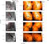 |
Fig. 1 Compilation of the continuum data from 70 μm to 1.1 mm wavelength for G28.34 S, IRDC 18530, IRDC 18306, and IRDC 18308. Left column: graymaps of the dust emission observed by Herschel at 70 μm (Ragan et al. 2012a). The red contours show continuum emission observed by ATLASGAL at 870 μm (Schuller et al. 2009), starting from 10σ rms and continuing in 10σ rms steps. Middle and Right columns: black contours show continuum observed by SMA COMP configuration (middle) and COMP+EXT combination (right), overlaying the moment 0 colormaps of H13CO+(1 → 0) (integrated through its velocity dispersion) from IRAM 30 m observations. COMP contours start from 5σ rms and continue in 5σ rms steps, while COMP+EXT contours start from 3σ and continue in 3σ steps. 1σ rms of each source configuration is listed in Table 3. Cyan letters mark the fragments having >3σ rms continuum emission in both COMP and COMP+EXT maps. In each panel of the middle and right columns, the SMA synthesized beam is in the bottom left. The cyan circles show the primary beam of SMA at 1.1 mm, and the black dashed circles show the beam of 30 m at 3 mm. |
3. Observational results
3.1. Fragmentation on small scale from SMA observations
As shown in Fig. 1, our sources locate on the ATLASGAL 870 μm continuum peaks of the pc-scale filaments (shown as red contours in the left column). All targets are embedded in the Herschel 70 μm dark clouds (Ragan et al. 2012a), and each of them is away from the 70 μm bright region at a projected distance of ~1–2 pc (1′–2′). At an angular resolution of ~2′′ (corresponding to 104 AU on linear scales), the 1.1 mm SMA observations resolve each 870 μm continuum peak into several compact substructures (hereafter “fragments”, plotted as black contours in the middle and right columns of Fig. 1). Combined with “natural weighting”, observations with the COMP+EXT configuration achieve a relatively high angular resolution, but high sensitivity only to the compact structures. Observations with the COMP configuration, however, achieve a higher signal-to-noise ratio and recover some extended structures of the envelope, so they are essential for studying the morphology of the fragments, e.g., size, mass.
We find 2–4 fragments per source with continuum emission levels >3σ rms in both the COMP and COMP+EXT maps. These fragments have typical sizes of 0.05–0.2 pc and masses of 4–62 M⊙. They are mostly separated at a projected distance of 0.07–0.24 pc (see Table 4 and discussion in Sect. 4.1). In particular, fragments in G28.34 S and IRDC 18308 are well aligned along the large-scale filamentary direction. The spatial resolution of our observations only allow the “core” structure to be resolved, so we cannot tell whether the cores contain further hierarchic fragments into condensations or stay as monolithic objects in this paper.
3.2. Line survey from IRAM 30 m at 1 mm/3 mm
Our target lines in the SMA observations included cold, dense gas tracers such as H13CO+ (3 → 2,Eu/kB = 25 K), H13CN (3 → 2,Eu/kB = 25 K), HN13C (3 → 2,Eu/kB = 25 K), and HNC (3 → 2,Eu/kB = 26 K). However, none of them has >4σ rms emission at 1.1 mm.Possible explanations for this include the following: (1) these species were tracing the more extended structures which our observations are not sensitive to; (2) their emission was too faint to detect, given the sensitivity of our SMA observations; or (3) these high-J lines were not yet excited in these young, cold HMSCs. Our new IRAM 30 m line survey now recovers the extended structure information with 3–10 times more sensitivity than the SMA observations. We now detect emission from lower-J transitions of the above species at 3 mm.
 |
Fig. 2 Averaged spectra from IRAM 30 m line survey at 3 mm/1 mm, which are extracted from a square region ([20′′, 20′′] to [−20′′, −20′′] offset) centered on the SMA continuum peak. The spectral resolution is 0.194 MHz (0.265 km s-1 at 1 mm and 0.641 km s-1 at 3 mm). All detected lines are labeled. The “extra band” is not shown here because of less integration time and thus there is a lower signal-to-noise ratio. |
3.2.1. Line identification
We present the spectra from each 30 m targeted source in Fig. 2. To increase the signal-to-noise ratio for the weak emission in the dark clouds, each spectrum is averaged from a square region ([20′′, 20′′] to [−20′′, −20′′] offset) centered on the SMA continuum peak (the mapping center of the 30 m observations). Using the Splatalogue database8, we identified 32 lines from 15 species (including 20 isotopologues) in the 16 GHz-broad 1 mm/3 mm band (Table A.1, the lines detected only in the extra band are in blue). Most of them are “late depleters”, which have low critical densities, low Eu/kB, and low binding energies, and thus are hard to deplete onto grain surfaces (Bergin 2003). Although IRDC 18306 is the nearest source in our sample, its lines have the lowest brightness temperatures. In contrast, G28.34 S has the largest number of detected lines with the highest brightness temperatures in our sample, indicating that this source may be chemically more evolved than the others in our sample.
3.2.2. Molecular spatial distribution
When a high-mass star-forming region (HMSFR) is in the early chemical stages, different species trace gas with different temperatures and densities. Therefore, the spatial distribution diversity from different species can tell us the chemical status of a particular host source.
From Fig. 2, G28.34 S has the largest number of emission lines, so we use this source for line identification and list all the detections (having emission >4σ rms) in Table A.1. The line profiles as plotted in Fig. A.1 show that some lines have blended multiplets. To account for this multiplicity when mapping the distribution of all identified species in each source, we integrate each line according to its detection and multiplet using the rules below.
If a line that has ≥4σ detection in a particular source contains a multiplet, we fit the strongest multiplet transitions using the hyperfine-structure (HFS) fit; otherwise, we fit it using a Gaussian profile9 (as discussed in Sect. 4.3.1 and listed in Table A.2)10. Subsequently, we map the integrated intensities of these lines over their velocity range (down to where the line goes into the noise, Table A.3).
If a G28.34 S-detection species has <4σ detection in another particular source, we integrate a total of three channels around the systematic Vlsr at the rest frequency of its strongest transition (marked with “*” in Table A.3) in that source.
Figure 3 presents the spatial distributions of all the detected species in our sample. We note that the intensity of some lines in the 70 μm bright sources in our field of view (~1′ NE to G28.34 S, IRDC 18530, and NW to IRDC 18308) are stronger than in our target 70 μm dark sources, which makes the spatial origin of these species hard to judge. Therefore, we plot the contour that marks the half maximum integrated intensity of a particular species (the black contours in Fig. 3). In general, most species show the strongest emission towards the 870 μm continuum peak. We note that molecular emission peaks in IRDC 18306 and IRDC 18308 have a systematic offset of ~5″–10″ north of the continuum peak. This may be caused by the pointing uncertainties between 30 m and APEX. Nevertheless, comparison among the sources reveals some similarities and special features of the species that we outline in greater detail for different types of chemistry. Figure A.1 shows the line profiles and Fig. 3 the distributions11.
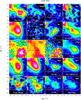 |
Fig. 3 Molecular line integrated intensity maps overlaid with the 870 μm continuum contours in G28.34 S, IRDC 18530, IRDC 18306, and IRDC 18308. The maps in each source are ordered in different groups according to line rest frequencies and the leading isotopes. Colormaps show the intensity integrations (K km s-1) over the velocity dispersion of each line. For the lines with <4σ detections, we only integrate a total of three channels around the system Vlsr at their rest frequencies. The purple contour in each panel indicates the area with integrated intensity >4σ rms. The black contour indicates the area within which integrated intensity is over the half maximum in the field of view. The white contours show the continuum emission from 870 μm ATLASGAL data, starting from 10σ and increasing by 10σ. |
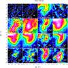 |
Fig. 3 continued. |
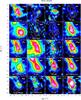 |
Fig. 3 continued. |
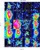 |
Fig. 3 continued. |
-
Nitrogen (N-) bearing species have the largest number of lines de-tected in our 30 m observations. Previous stud-ies especially towards low-mass star-forming regions (e.g., Leeet al. 2001; Pirogovet al. 2003; Fulleret al. 2005; Raganet al. 2006; Sanhuezaet al. 2012; Fontaniet al. 2014) show that these speciesusually trace the cold, dense gas because of their large dipole mo-ments, relatively low optical depths, or simple linear structures(e.g., HC3N, Bergin et al. 1996). Among them, the abundance of NH2D can be enhanced by deuteration from NH3 (
 ) when CO has frozen out onto the dust grains (T< 20 K, Crapsi et al. 2005; Chen et al. 2010; Pillai et al. 2011); HCN (H13CN) is a well-known infall tracer in low-mass prestellar environment (e.g., Sohn et al. 2007); the ratio of HCN/HNC (H13CN/HN13C) is strongly temperature dependent, high in the warmer region like Orion GMC (Goldsmith et al. 1986; Schilke et al. 1992) and approximately around unity (Sarrasin et al. 2010) in the cold environment (see discussion in Sect. 4.4); multiplets of N2H+ are commonly used to reveal the excitation temperature of this species (e.g., Caselli et al. 2002a) in the dark, quiescent regions. All these species have emission peaks or strong emission coincident with the 870 μm continuum peaks, and the offsets between them are less than the pointing uncertainty between 30 m and APEX. In particular, isotopologues of HNC and HCN are co-spatial in sources except for HCN (H13CN) in IRDC 18308. This exception may be explained by the abnormal enhancement or suppression of the individual hyperfine line discussed in Sect. 4.3.1, indicating non-LTE (local thermal equilibrium) excitations of HCN (Loughnane et al. 2012).
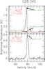
Fig. 4 Asymmetric line profile of HCO+(1 → 0) compared to H13CO+(1 → 0) in G28.34 S, indicating infall motion with a speed of ~0.84 km s-1.
In addition to the simple N-bearing species, HNCO is the simplest organic species containing C, H, O, and N elements. Moreover, it has been suggested as a shock tracer, based on its correlated spatial distribution with SiO (e.g., Zinchenko et al. 2000) and CH3OH (e.g., Meier & Turner 2005). We found extended emission of HNCO in all our dark, cold clumps. The velocity dispersion of this line is similar to the other lines (1–3 km s-1) on the scale of 0.8 pc, so we are not able to tell whether the shocks are from cloud-cloud collision (e.g., Jiménez-Serra et al. 2009, 2010; Nguyen-Lu’o’ng et al. 2013) or from protostellar objects deeply embedded.
-
Carbon oxidized and hydride species are important indicators of the chemical status of a particular star-forming region. Because they are one of the most abundant molecules in the gas phase, possessing a low dipole moment and low critical density, CO isotopologues (13CO, C18O, and C17O) can be used to indicate the gas temperature (e.g., Tafalla et al. 1998; Pineda et al. 2008, see also Appendix B). HCO+ is the typical dense gas tracer produced from CO, and its abundance is enhanced in regions with a high ionization fraction and/or shocked by outflows (e.g., Codella et al. 2001; Hofner et al. 2001; Rawlings et al. 2000, 2004). H2CO is an important carbon hydride which forms CH3OH and other more complex organics later in the gas phase (e.g., Horn et al. 2004; Garrod et al. 2008); sublimation of this species needs a warmer environment, so the detection of this species indicates the host cloud may be in a more evolved phase. These species show the following features in G28.34 S: (1) a clear anti-correlated distribution between CO isotopologues (especially the optically thin 2 → 1 lines of C18O and C17O) and N2H+/NH2D/H13CO+, indicating strong depletion and ionization even on the scale of 0.8 pc (see discussion in Sect. 4.5); (2) a blue asymmetric line profile of the optically thick HCO+ (1 → 0) comparing to H13CO+ (1 → 0), indicating possible large velocity of infall motion (Myers et al. 1996; Mardones et al. 1997, see Fig. 4 and Sect. 4.3 for detailed discussion); and (3) >4σ line emission from H2CO coincident with the continuum peak, indicating warmer gas there. Despite a tentative anti-correlated distribution between C17O and N2H+/H13CO+ on the scale of 0.5 pc in IRDC 18308, a 10′′ (0.2 pc) offset between CO and NH2D emission peak in IRDC 18308, and a tentative detection of H2CO (2σ emission) in IRDC 18306, the other sources do not have the same features found in G28.34 S. We note that the emission peak of HCO+ (1 → 0) and H13CO+ (1 → 0) are not strictly co-spatial in any source (offsets are 5″−10″), and this may come from the large opacity of HCO+. However, H13CO+ shows a “deficiency” at the continuum peak of IRDC 18530 where 13CO is abundant, which is probably due to the dissociative recombination in this environment (see discussion in Sect. 4.6).
-
SiO is a typical shocked gas tracer, and is commonly associated with one or more embedded, energetic young outflows. We detect SiO (2 → 1) only in G28.34 S, where this line shows strong emission and broad line wings (Fig. A.1). Coincident with the H2O maser in G28.34 S (Wang et al. 2006), its emission may be from outflow and thus implies that a protostar is already embedded in this source. However, we cannot rule out the possibility that the SiO emission may also come from the bright infrared source which is 40′′ south of our targeted region, or from G28.34 P1 which is 1′ to the north and hosts several jet-like outflows (Wang et al. 2011; Zhang et al. 2015). Therefore, the spatial origin of SiO is crucial to diagnose the evolutionary status of G28.34 S, and thus further kinetic study with higher sensitivity data12 is needed to confirm its spatial origin.
-
Carbon chains/rings are a mysterious group of species whose gas/grain origin is still not clear. Among the species we detected, C2H is thought to reside (predicted by chemical models) in the source center in the early stage, before transforming into other species (e.g., CO, OH, H2O), and it can have high abundance in the outer shells even at later stages (Beuther et al. 2008); the carbon ring c-C3H2, first detected in the cold dark cloud TMC-1 by Matthews & Irvine (1985), is reported to survive even in a hot region where NH3 is photon-destroyed (Palau et al. 2014); and CH3C2H is considered a good probe of temperature for early stages of star-forming regions (Bergin et al. 1994). We detect the above-mentioned carbon chains/ring towards the continuum peak of all our sources, except in IRDC 18530 where only C2H is observed. However, since these species also show stronger or roughly the same emission towards the nearby 70 μm bright sources (according to the half maximum intensity contour), we cannot tell whether these species are good cold gas tracers or not.
-
Sulfur (S-) bearing species also have unknown chemistry. Two S-bearing lines, 13CS(2 → 1) and OCS (7 → 6) are covered in our observations (except for the OCS line in IRDC 18530). Owing to their high dipole moments, CS isotopologues are used as dense gas tracers (e.g., Bronfman et al. 1996) in both low-mass (e.g., Tafalla et al. 2002) and high- mass prestellar cores (e.g., Jones et al. 2008), but they show high depletions in the center of high-mass dense cores (e.g., Beuther & Henning 2009). OCS forms via surface chemistry and is the only S-bearing molecule that has actually been observed on interstellar ices (Palumbo et al. 1997). Both 13CS and OCS are only detected in G28.34 S with >4σ emission, but these emissions have been shown to originate from the NE bright source, according to their half maximum intensity contours. Therefore, we do not claim their spatial origin from the cold gas.
In short, G28.34 S appears chemically more evolved than the other sources in our sample, thanks to the sole detections of H2CO and OCS, the strong emission of HNCO, the HCO+ asymmetric line profile implying significant infall, and SiO coinciding with previous H2O maser detection. All these signatures indicate that G28.34 S is the host of potential protostellar objects.
4. Analysis and discussion
4.1. Fragmentation
Figure 1 presents the continuum maps of Herschel 70 μm, APEX 870 μm (ATLASGAL), and SMA 1.1 mm. Because the COMP+EXT configuration of SMA filters out some extended structures, in the following we calculate parameters using data obtained with the COMP configuration only.
We assume that the dust emission is optically thin, and that dust is fully coupled with gas with the same temperature. Therefore, we estimate the mass Mfr and column density Nfr in the resolved fragments from the SMA continuum maps with (Hildebrand 1983; Schuller et al. 2009): 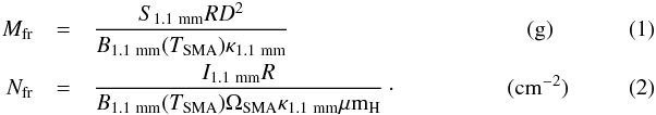 The averaged column density of the entire clump (in the 40″ × 40″ region) Nc can be estimated from each ATLASGAL continuum map as well,
 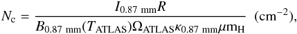 (3)where D is the source kinematic distance (from the Sun), S1.1 mm is the total continuum flux density at 1.1 mm (measured from each fragment after a 2D Gaussian fit13, in units of Jy); I1.1 mm is the specific intensity for the continuum peak of each fragment (in Jy beam-1); I0.87 mm is the averaged specific intensity in the 40″ × 40″ region (in Jy beam-1); R is the isothermal gas-to-dust mass ratio (taken to be 150, from Draine 2011), B1.1 mm(TSMA) and B0.87 mm(TATLAS) are the Planck functions for a dust temperature TSMA or TATLAS; ΩSMA and ΩATLAS are the solid angles of the SMA and ATLASGAL beam (in rad2); κ1.1 mm = 1.0 cm2 g-1 and κ0.87 mm = 1.8 cm2 g-1 are the dust absorption coefficients at 1.1 mm and 870 μm (assuming a model of agglomerated grains with thick ice mantles for densities105–106 cm-3, extrapolated from Ossenkopf & Henning 1994); μ is the mean molecular weight of the ISM, which is assumed to be 2.33; and mH is the mass of a hydrogen atom (1.67 × 10⁻²⁴ g).
As described in Table 4, the sizes of fragments (from 2D Gaussian fitting) are 2–4 times larger than the SMA beam size on small scales. On larger scales, the sizes of filamentary structures (projected area with >10σ emission) seem to be more extended than the primary beam of ATLASGAL (θALTLASGAL = 18″). Therefore, we take the filling factors as unity in both spatial scales.
The parameters measured from SMA observations at 1.1 mm, including the coordinates, specific intensity at continuum peak, total flux density, and projected source size.
Firstly, we compare the gas concentrations on different spatial scales. Following Kirk et al. (2006), assuming Bonner-Ebert (BE) spheres for both large-scale clumps and small-scale cores, the gas concentration can be estimated in terms of observable parameters as ![Mathematical equation: \begin{eqnarray} \rm Con_{ATLAS}&=&\rm 1-\frac{1.44\Omega_{ATLAS}}{{\it I}_{\rm 0.87~mm}}\overline{\frac{{\it S}_{\rm 0.87~mm}}{{\it A}_{\rm 0.87~mm}}} \label{irdc:conc_atlas} \\[4mm] \rm Con_{SMA}&=&\rm 1-\frac{1.44\Omega_{SMA}{\it S}_{\rm 1.1~mm}}{{\it A}_{\rm 1.1~mm}{\it I}_{\rm 1.1~mm}}\cdot \label{irdc:conc_sma} \end{eqnarray}](/articles/aa/full_html/2016/08/aa26864-15/aa26864-15-eq215.png) Here A1.1 mm is the size of each small-scale fragment derived from 2D Gaussian fits (almost the same size as the area within the 5σ continuum contour). Since ATLASGAL filaments are not suitable to fit with a 2D Gaussian, we measure the total flux per unit projection size on each ATLASGAL clumps (
Here A1.1 mm is the size of each small-scale fragment derived from 2D Gaussian fits (almost the same size as the area within the 5σ continuum contour). Since ATLASGAL filaments are not suitable to fit with a 2D Gaussian, we measure the total flux per unit projection size on each ATLASGAL clumps ( ) with the following approach. Following Wang et al. (2015), we extract a flux intensity profile from a cut perpendicular to the filament elongated direction, which is centered on the mapping center of the 30 m observations14. Then we measure the FWHM width of the filament locally around our source. For each filament, we set three rectangles along the filamentary orientation. These rectangles all have the same centers as the previous cut and the same width as the local FWHM width. The length of the rectangles along the filament are one, two, and three times of the FWHM width. Then, we measure the total flux and projection size within each rectangle and derive the mean.
We find that the gas concentration (listed in Tables 4 and 5) on large scales (ConATLAS ~ 0.6) is lower than that in the small-scale fragments (ConSMA ~ 0.8). Moreover, the large-scale concentration is on the verge of requiring additional non-thermal support mechanism (critical value of BE sphere as 0.72 from Walawender et al. 2005; Kirk et al. 2006).
Secondly, assuming that all small-scale fragments and large-scale cloud clumps are spherically symmetric, we then estimate the gas volume number density of each fragment nfr from θSMA (in units of rad), and the averaged gas volume number density nc of the entire clump on larger scales from θALTLASGAL (in units of rad) as15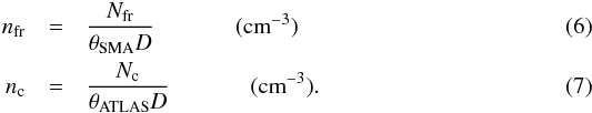 We assume that the core-scale structures (size of ~0.1 pc) seen in the SMA-COMP configuration result from the fragmentation from the pc-scale clumps. If fragmentation is governed by the thermal Jeans instabilities, the thermal Jeans length λth−J and mass Mth−J of the entire clump can be estimated from the averaged density and temperature in this clump,
  where G is the gravitational constant (6.67 × 10⁻⁸ cm3 g-1 s-2) and cs = [kBTATLAS/ (μmH)] 1/2 is the speed of sound at temperature TATLAS.
Parameters from 30 m and APEX observations and estimates based on two hypotheses of fragmentation (thermal Jeans fragmentation and turbulent Jeans fragmentation).
We assume TSMA = 15 K for the following reasons: (1) we did not detect the SMA-targeted lines with low upper energy levels (Eu/k ~ 25 K); (2) low temperatures have been estimated from other observations in G28.34 S, including the SABOCA 350 μm survey (13 K as upper limit, 11′′ resolution; Ragan et al. 2013), SPIRE 500 μm observations (16 K, 36′′ resolution), and the rotation temperature of NH3 derived from VLA+Effelsberg (13–15 K, 5′′ resolution, Wang et al. 2008; priv. comm. with K. Wang); (3) it is unclear whether a protostar has already formed in these sources. Dust and gas may either have higher temperature in the envelope region (i.e., structures probed by ATLASGAL, SABOCA, and SPIRE 500 μm) than at the SMA-probed center because of UV-shielding, or the envelope can be colder than the central core if the protostar has formed (i.e., in G28.34 S). In either case, we give the estimates of the large-scale ATLASGAL clumps at ad hoc temperatures 12 K, 15 K, and 18 K.
As shown in Tables 4 and 5, the volume number densities in the SMA fragments are at least ten times higher than the averaged volume number densities found in the ATLASGAL clumps. Moreover, the average projected separation between the fragments (0.07–0.24 pc) is comparable to the predicted thermal Jeans length of the entire clump (0.07–0.18 pc) at a temperature of TATLASGAL> 12 K and TSMA ~ 15 K. However, the fragment masses are significantly higher (more than four times) than the predicted thermal Jeans masses of the entire clumps, even without accounting for interferometric-filtering. In particular, fragment masses are >10M⊙ in our sample, except for IRDC 18530. A similar discrepency has also been reported in fragmentation studies in several other IRDCs (e.g., Wang et al. 2014; Beuther et al. 2015).
Different hypotheses have been proposed for the “non-thermal support”, as listed below.
Turbulent Jeans fragmentation Since thermalJeans fragmentation describes the fragmentation processeswhen the internal pressure is dominated by the thermal motion,the above-mentioned discrepency indicates that non-thermalmotions, such as turbulence may play an important role infragmentation (e.g.,Wanget al. 2011, 2014). To investigate whether non-thermal pressure provides extra kinetic energy against the gravitational energy of the fragments, we need to measure the velocity dispersion over the entire clump, which can be derived from the linewidth of the dense gas tracer(s). The linewidths of all the species are on average 2–3 km s-1 (see Table A.2). H13CO+ (1 → 0) has a high critical density (ncrit> 104 cm-3; Bergin & Tafalla 2007; Csengeri et al. 2011; Shirley 2015), low Eu/kB (4 K), and no hyperfine multiplet. Its velocity dispersion is not affected by Galactic spiral arms (e.g., the line profiles of CO, C18O, and C17O along the line of sight are contributions from various Galactic arms; see Beuther & Sridharan 2007), and it has a symmetric Gaussian profile. Therefore, we use this line to measure the observed velocity dispersion in the line of sight
 . Here we assume that the averaged gas temperature in the entire clump is T30 m = TATLAS. Comparing σobs with the thermally broadened velocity dispersion of H13CO+
 , we estimate the non-thermally broadened velocity dispersion
  (see Table 5). Within the gas temperature T30 m range of 12–18 K, we find that σobs is dominated by non-thermal motions throughout the entire source clump (size of ~105 AU). Therefore, assuming that turbulence dominates the non-thermal motion, we replace cs with σobs in Eqs. (8) and (9) and list the turbulent Jeans length λNth−J and mass MNth−J in Table 5:
 ![Mathematical equation: \begin{eqnarray} \lambda_{\rm Nth-J}&= &\sigma_{\rm obs}\left(\frac{\pi}{G\mu m_{\rm H}n_{\rm c}}\right)^{1/2} \nonumber\\[2mm] &=& \rm 0.35\left(\frac{\sigma_{\rm obs}}{\rm km\,s^{-1}}\right)\left(\frac{{\it n}_{\rm c}}{10^5\,{\rm cm}^{-3}}\right)^{-1/2}\,{\rm pc} \label{irdc:tur_l} \\[2mm] M_{\rm Nth-J}&=& \frac{\sigma_{\rm obs}^3}{6}\left(\frac{\pi^5}{G^3\mu m_{\rm H}n_{\rm c}}\right)^{1/2} \nonumber\\[2mm] &=&\rm 136.33\left(\frac{\sigma_{\rm obs}}{\rm km\,s^{-1}}\right)^{3}\left(\frac{{\it n}_{\rm c}}{10^5\,{\rm cm}^{-3}}\right)^{-1/2}\,{\it M}_{\odot} \label{irdc:tur_m} . \end{eqnarray}](/articles/aa/full_html/2016/08/aa26864-15/aa26864-15-eq356.png) The above equations do not take magnetic fields into account.In such a regime, the non-thermal motions provides sufficient extra support in the cloud even at low temperatures, and may increase the fragmentation scale. Both λNth−J and MNth−J are higher than the values observed with SMA, and so this may be a viable method of support. Of course it should be noted that, if the turbulence lead to shocks occurring in the region, the increased density may lead instead to further fragmentation (Dobbs et al. 2005). Note that our data is insufficient to isolate multiple velocity components, given its spectral and spatial resolution. If these are present, the velocity dispersion, and therefore turbulent Jeans length/mass, would be overestimated.The large-scale filamentary gas distribution at 870 μm and the small-scale SMA fragments in G28.34 S and IRDC 18308 are well aligned with roughly the same projected separation (Fig. 1). Similar feature has been reported in other HMSFRs, e.g., G28.34 S P1 (Zhang et al. 2009; Wang et al. 2011), G11.11–0.12 (Wang et al. 2014), and NGC 7538 S (Feng et al. 2016). Simulations (e.g., Chandrasekhar & Fermi 1953; Nagasawa 1987; Bastien et al. 1991; Inutsuka & Miyama 1992; Fischera & Martin 2012) also predicted that isothermal, “cylindrical” gas collapses into a chain of fragments, with equal spatial separation λcl along the filament under self gravity, and then the fragments grow due to “varicose” or “sausage” fluid instability (Jackson et al. 2010). Without magnetic fields, the critical linear mass density (M/l)crit represents the linear mass over which self-gravity overcomes the internal thermal and non-thermal pressure. The critical separation λcl and critical mass of fragment Mcl in the large-scale clump were originally given in Chandrasekhar & Fermi (1953), Nagasawa (1987). In the case that the thermal motions are not sufficient to be against gravitational energy, we replace the sound speed with the velocity dispersion σobs, and have (Fiege & Pudritz 2000; Wang et al. 2014):
The above equations do not take magnetic fields into account.In such a regime, the non-thermal motions provides sufficient extra support in the cloud even at low temperatures, and may increase the fragmentation scale. Both λNth−J and MNth−J are higher than the values observed with SMA, and so this may be a viable method of support. Of course it should be noted that, if the turbulence lead to shocks occurring in the region, the increased density may lead instead to further fragmentation (Dobbs et al. 2005). Note that our data is insufficient to isolate multiple velocity components, given its spectral and spatial resolution. If these are present, the velocity dispersion, and therefore turbulent Jeans length/mass, would be overestimated.The large-scale filamentary gas distribution at 870 μm and the small-scale SMA fragments in G28.34 S and IRDC 18308 are well aligned with roughly the same projected separation (Fig. 1). Similar feature has been reported in other HMSFRs, e.g., G28.34 S P1 (Zhang et al. 2009; Wang et al. 2011), G11.11–0.12 (Wang et al. 2014), and NGC 7538 S (Feng et al. 2016). Simulations (e.g., Chandrasekhar & Fermi 1953; Nagasawa 1987; Bastien et al. 1991; Inutsuka & Miyama 1992; Fischera & Martin 2012) also predicted that isothermal, “cylindrical” gas collapses into a chain of fragments, with equal spatial separation λcl along the filament under self gravity, and then the fragments grow due to “varicose” or “sausage” fluid instability (Jackson et al. 2010). Without magnetic fields, the critical linear mass density (M/l)crit represents the linear mass over which self-gravity overcomes the internal thermal and non-thermal pressure. The critical separation λcl and critical mass of fragment Mcl in the large-scale clump were originally given in Chandrasekhar & Fermi (1953), Nagasawa (1987). In the case that the thermal motions are not sufficient to be against gravitational energy, we replace the sound speed with the velocity dispersion σobs, and have (Fiege & Pudritz 2000; Wang et al. 2014):  In Table 5, we list the critical mass and separation of each source estimated from cylindrical fragmentation. Non-thermal motions, such as turbulence in this special case, can provide support against gravitational collapse of the mass up to ~800 M⊙. In particular, the hypothesis of cylindrical fragmentation predicts high linear mass densities for both G28.34 S (788 M⊙ pc-1) and IRDC 18308 (365 M⊙ pc-1), which are similar to that of IRDC G11.11-0.12 found in Kainulainen et al. (2013) and Wang et al. (2014).These predictions are upper limits, because possible unresolved velocity components may lead to an overestimation of the H13CO+ velocity dispersion from the 30 m observations (at the angular resolution of 30′′). To compare the predicted upper limit with the values from observations, we also measure the linear mass of the above ATLASGAL filamentary clumps (M/l)ATLAS from their dust emission maps16 at the angular resolution of 18′′. We find that if G28.34 S is warmer than 18 K (855 ± 244 M⊙ pc-1) and IRDC 18308 is warmer than 15 K (265 ± 23 M⊙ pc-1, Table 5), the predicted upper limits are higher than the observed linear mass of the ATLASGAL sources. If magnetic field were taken into account, the predicted linear mass would be even higher (e.g., Kirk et al. 2015), i.e., both clumps are likely stable against cylindrical fragmentation.
-
Other possibilities We do not find obvious velocity gradients in our sources, so the rotation energy is negligible compared to the gravitational energy17. Nevertheless, other factors in addition to non-thermal motions may also lead to a “mass/separation discrepancy” between the observations and thermal Jeans predications, where the projected separation between the fragments are comparable to the Jeans length, but the observed mass is higher than the Jeans mass. The possible factors are the following:
(1): Magnetic fields may suppress fragmentation (e.g.,Commerçon et al. 2011).
(2): An inhomogeneous density profile in the core may alter its fragmentation properties. For example, recent numerical simulations by Girichidis et al. (2011) show that less fragmentation occurs in steeper initial density profiles, and the final fragments are more massive than from a flat initial density profile (by a factor of up to 20 in the extreme case).
(3): The “precise” Jeans length is difficult to quantify. Since the sensitivity of the SMA observations does not detect lower mass fragments, the separation between the fragments is an upper limit of the Jeans length. Conversely, the projection of a 3D distribution onto the plane of the sky reduces the observed fragment separation, which makes the measured length a lower limit of the Jeans length. It is difficult to assess quantitatively how these two factors affect the measured separation between dust peaks. These uncertainties make the Jeans length comparison problematic.
(4): As the density increases, the local Jeans mass decreases, cores can fragment further. Therefore, based on the current data, we cannot rule out the possibility of unresolved internal sub-fragments (condensations).
In short, the mass of the initial fragments resolved from 1.1 mm SMA observation are already high (on average >10 M⊙). Thermal energy alone cannot compete against the self-gravity of these fragments; however, the combination of thermal and non-thermal motions can provide sufficient energy in opposing the further fragmentation. Moreover, a steep initial density profile of the entire clump and the magnetic field may also increase the upper limit of the final fragment mass. With the current data, it is difficult to measure the precise Jeans length and resolve internal substructures in the fragments. Therefore, we cannot differentiate between the above scenarios.
4.2. Infall motion
We find that the line profiles of HCO+ (1 → 0), which is likely optically thick, shows an asymmetric non-Gaussian profile, especially in G28.34 S. In contrast, H13CO+ (1 → 0), which is optically thin, shows a fairly symmetric profile (Fig. 4). Following Mardones et al. (1997), we measure the normalized velocity difference between the two lines δVH13CO+ = (VHCO+−VH13CO+)/ΔυH13CO+ in each source. Except for IRDC 18308, δVH13CO+ in other sources are significant18 (Table 8), indicative of violent dynamics. In particular, line profile of HCO+ (1 → 0) in G28.34 S shows double intensity peaks of blue- and redshifted gas, indicating a potential infall motion, with an infall speed ~0.84 km s-1 (derived by using Eq. (9) of Myers et al. 1996). Nevertheless, we note that the peak intensity of the redshifted gas is only 0.1 as strong as that of the blueshifted gas, so we cannot rule out the possibility that double intensity peaks comes from multiple velocity components. If this is the case, the high-velocity (redshifted) gas of H13CO+ (1 → 0) may be too weak for the observation sensitivity.
4.3. Molecular column density and abundance estimates
We did not detect emissions of the higher-J molecular transitions in the fragments from the SMA observations. However, the lower-J transitions of the dense gas tracers are detected in the extended structures in the 30 m line survey. This indicates that our sources are in the cold, young phase. To probe the chemical properties in these gas clumps, we quantify their excitation conditions and molecular abundances in this section.
4.3.1. Molecular excitation temperatures and column densities
We calculated the molecular column densities averaged from the central 40′′ × 40′′ region of each source. Since the optical depth may lead to large uncertainties of certain lines, we use different methods to correct their opacities.
N2H+,C2H, HCN, and H13CN have multiplets in theirJ = 1 → 0 or N = 1 → 0 (C2H) transitions. We use the HFS method to fit these transitions (Fig. 5) and list their excitation temperatures Tex in Table 6 (see Appendix A for details). From the fits, we find that the linewidths of the strongest components Δυ of the above species are in the range of 1.7–3.2 km s-1. This is consistent with the linewidths of the other species (Table A.2), indicating that non-thermal motions dominate the velocity dispersion. N2H+ (J = 1 → 0) and C2H+ (N = 1 → 0) are fitted very well, but the fits for HCN (J = 1 → 0) and H13CN (J = 1 → 0) show strong deviations. Most of the Tex we derived from the HFS fits are below 10 K (except for HCN in G28.34 S), which could be due to multiple factors:
(1): In the cold gas environment with densities of104–105 cm-3, species with high critical densities are subthermally excited (e.g., at 10 K, the critical density of N2H+ (J = 1 → 0) is ~6 × 104 cm-3, and that of HCN (J = 1 → 0) is ~5 × 105 cm-3; Shirley 2015), so their Tex is lower than the typical kinetic temperatures of IRDCs (e.g., Sridharan et al. 2005; Vasyunina et al. 2011; Fontani et al. 2012). This feature is common in both high-mass and low-mass dark clouds (e.g., Caselli et al. 2002b; Crapsi et al. 2005; Miettinen et al. 2011; Fontani et al. 2012).
(2): To increase the signal-to-noise ratio for the weak emission, we extract the average spectra from the 40′′ × 40′′ region, but the gas is not homogeneous as assumed. For one thing, H13CN is deficient at the continuum peak of IRDC 18530 and IRDC 18308 (Fig. 3). In addition, HCN (J = 1 → 0) has an anomalous line profile in IRDC 18306 (the HFS component with the strongest relative intensity shows weaker emission than the others). This “anomalousness” has also been noted by Afonso et al. (1998) and was explained as the inconsistency intensity ratios between multiplets of HCN, i.e., individual hyperfine lines may be enhanced or suppressed in dark clouds because of non-LTE (Loughnane et al. 2012). Therefore, the low Tex we derive here are the averaged excitation temperatures from the imperfectly fitted spectrum (Fig. 5.III).
(3): The HFS method is applicable when the source is in ideal LTE (assumption 1–3 in Appendix A) and multiplets are resolved (assumption 4). However, in our observations HCN and H13CN may be non-LTE, and seven multiplet lines of N2H+ are blended into three Gaussian peaks at a velocity resolution of ~0.641 km s-1 (Fig. 5.I). Therefore, the HFS method only gives the rough level of the Tex.
(4): Another factor which would affect the Tex estimation is the filling factor f, which is estimated by assuming that the species emission extent is equal to the area within the contour of half maximum integrated-intensity (Eq. (A.1)–(A.3)). In most cases, the emission extends over the 30 m primary beam, so f ~ 1. For species whose equivalent distribution diameter is smaller than the primary beam could have a f ≪ 1 (e.g., H13CN in IRDC 18306 and IRDC 18308 have f< 0.5). Moreover, the asymmetric spatial distribution of emission would also bring uncertainty (i.e., the equivalent distribution diameter depends on the velocity range we integrate and the edge of the emission extent we define). On average, Tex is underestimated for f ~ 1 and will increase by a factor of 1.2–1.5 for f ~ 0.2.
Following the “CTex” approach introduced by Caselli et al. (2002c), where N2H+ with Tex ~ 5 K, we assume that the transitions of each molecule can be described by an approximately constant Tex. Then we estimate the column densities of the above species19 with Eq. (A.4).
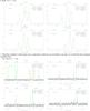 |
Fig. 5 Hyperfine multiplet fits (green lines) to the observed N2H+ (J = 1 → 0), C2H (N = 1 → 0), HCN (J = 1 → 0), and H13CN (J = 1 → 0) (black histograms) from each IRDC; the fit parameters are in the right upper corner. The transitions of multiplets are labeled in the panels of G28.34 S (with the strongest line in red). |
 |
Fig. 4 continued. |
Tex derived from hyperfine fits to N2H+, C2H, HCN, and H13CN multiplets in four IRDCs.
Molecules without hyperfine multiplet CO isotopologues are important gas tracers because of their low dipole moments and thermalization near their critical densities (at 10–20 K, ~103 cm-3 for 13CO (2 → 1), ~104 cm-3 for C18O (2 → 1) and C17O (2 → 1)). Therefore, they are in LTE in our dense gas clumps (n = 104–105 cm-3), and their Tex can be taken as the Tkin of the gas.
Lower-J transitions of the CO isotopologues (e.g., 13CO (2 → 1)) may be optically thick, so a precise estimation of its Tex needs opacity correction. Assuming that fractionation (isotopic exchange reaction) of 12C ⇔ 13C and of 17O ⇔ 16O ⇔ 18O are stable, we correct the optical depth τ and estimate Tex of CO isotopologue (1 → 0) lines (listed in Table 7, see Appendix B for details).
CO depletion, HNC/HCN ratio, lower limit of ionization, and velocity asymmetric degree of H13CO+ in four IRDCs.
For G28.34 S and IRDC 18306, C18O (2 → 1) is optically thin according to our optical depth measurements from C17O (2 → 1) (Table 7). Since we did not observe C17O (1 → 0) in IRDC 18530, and the intensity of this line is only ~3σ rms in IRDC 18308, we take the optically thin C18O (2 → 1) as a standard to estimate the other chemical parameters.
The values of Tex derived from CO isotopologues are consistent in G28.34 S (11–14 K), indicating that CO is in LTE. This temperature range is also consistent with the values derived from VLA+Effelsberg NH3 observations, the SABOCA 350 μm survey, and SPIRE 500 μm observations (mentioned in Sect. 4.1). Most of the other lines without hyperfine multiplets have low critical density (except for SiO (2 → 1)), so we assume they are coupled with dust and thermalized at Tgas = Tdust = Tkin ~ Tex,CO. The column densities of these species can be derived according to Appendix C. In particular, the column densities of species whose rare isotopologue lines we detected (HCO+, HNC, and 13CO) are derived after opacity corrections.
Molecular column densities estimated using the above approaches are listed in Tables A.4 and A.5.
4.3.2. H2 column density estimates
It is possible to estimate H2 column density at clump-scale from Eq. (3). At the temperature of TATLAS = Tex,CO ~ 10 K, average H2 column density measured from the ATLASGAL in the 40″ × 40″ region is on the order of 1023 cm-2 (1 g cm-2, Table 8), which is consistent with the threshold for high-mass star-forming clouds proposed by Krumholz & McKee (2008).
4.3.3. Molecular abundance with respect to H2
APEX has a comparable beam size (18′′) to the IRAM 30 m at 1 mm (12′′) and 3 mm (30′′) . Therefore, assuming that the averaged continuum specific intensity at 18′′ angular resolution (from APEX) is comparable to that at 12′′–30′′ resolution (from the 30 m), the average molecular abundances with respect to H2 at the clump scale (within 40″ × 40″ region) can be estimated (Tables A.4 and A.5). One needs to keep in mind that the difference in the beam size will lead to the overestimation of the 1 mm molecular abundance and underestimation of the 3 mm molecular abundance by a factor of 2–3 because the H2 column density (Eq. (3)) is underestimated at 1 mm and overestimated at 3 mm.
The column densities of N2H+, C2H, HCN, and H13CN are estimated with respect to Tex estimated from their HFS fittings. Since Tex is different from that of the dust temperature used to derive the H2 column density, it introduces a large uncertainty for the column density estimates. Previous molecular spectral line observations towards several IRDCs have shown the typical range of Tkin = 10–20 K (e.g., Carey et al. 1998; Teyssier et al. 2002; Sridharan et al. 2005; Pillai et al. 2006; Sakai et al. 2008; Devine et al. 2011; Ragan et al. 2011; Zhang & Wang 2011). In addition, spectral energy distributions of clumps within “quiescent” IRDCs indicate a range of dust temperature Tdust = 10–30 K (e.g., Henning et al. 2010; Rathborne et al. 2010). Therefore, we also estimate the column densities and abundances of N2H+, C2H, HCN, and H13CN at the same Tkin ~ Tex,CO as the other species (see Table A.4). Comparison between the values at these two sets of temperatures indicates that the molecular abundances are sensitive to the temperatures in the 5–15 K regime, and 5 K difference in temperature brings the abundance uncertainty to the order of 1–2 mag. In the following analysis, we use the abundances at ~Tex,CO to estimate the other chemical parameters.
4.4. Chemical similarity and diversity of our sample compared to other HMSCs
On the clump-core scale (~0.8 pc), most strong emission lines detected by the 30 m observations are from N-bearing species, which show anti-correlation spatial distribution with CO isotopologues in G28.34 S and IRDC 18308. Emissions from shock tracers (e.g., SiO in G28.34 S and HNCO), infall tracers (e.g., HCO+ and HCN), and the detection of carbon ring (e.g., c-C3H2) indicate that these cold, young clouds are not completely “quiescent”.
Although the above features are qualitatively similar to the low-mass prestellar objects (LMPO) (typical scale of ~0.02 pc, Ohishi et al. 1992; Jørgensen et al. 2004; Tafalla et al. 2006), quantitative comparison between HMSCs and LMPOs requires observations on the same spatial scale. We compare the molecular abundances in our sources with previous spectral line studies in other HMSCs (e.g., Vasyunina et al. 2009; Gerner et al. 2014). On the one hand, all species in our sources have, on average, lower abundances than the above-mentioned studies, probably owing to our lower20Tkin and the possibly overestimated H2 column density (Sect. 4.3.3). Therefore, a more precise estimation of the molecular abundance requires a more reliable temperature measurement. On the other hand, species have higher abundances in G28.34 S than the others in our sample, again indicating that it is a chemically more evolved source.
The typical dense gas tracers HCN and HNC are a pair of isomers whose abundance ratio is strongly temperature dependent. It has been reported that the HCN/HNC ratio decreases with increasing temperature, ranging from ≤1 in the low-mass prestellar cores (e.g., Ohishi et al. 1992; Jørgensen et al. 2004; Tafalla et al. 2006; Sarrasin et al. 2010) to the order of unity in dark clouds (e.g., Hirota et al. 1998; Vasyunina et al. 2011), then above 10 in high-mass protostellar objects (e.g., Blake et al. 1987; Helmich & van Dishoeck 1997), and reaching several tens in warm cores (e.g., Orion GMC, Goldsmith et al. 1986; Schilke et al. 1992). In our sources, the HCN/HNC ratio is almost unity in G28.34 S and IRDC 18530 (Table 8), which is consistent with the value in dark clouds. If we compare the abundance ratio in our study to the statistical criteria value given by Jin et al. (2015), IRDC 18530 is likely a “quiescent” IRDC, and G28.34 S is more “active”.
4.5. CO depletion
The sublimation temperature of CO is around 20 K (Caselli et al. 1999; Fontani et al. 2006; Aikawa et al. 2008), so most CO is frozen out (depleted) onto the grains in the center of cold cloud. In contrast, N-bearing species are more resilient to depletion (e.g., Bergin et al. 2002; Caselli et al. 2002c; Jørgensen et al. 2004). Moreover, since CO destroys N2H+ and decreases the deuterium fraction, the anti-correlated spatial distribution between N2H+/NH2D and CO in G28.34 S and IRDC 18308 indicates strong depletion of CO (Fig. 3).
The depletion factor is defined as the ratio between the expected abundance of a species  and the observed abundance of that species
  (Lacy et al., 1994),
  . We measure the CO depletion factor averaged in the 40″ × 40″ region from J = 2 → 1 lines of C17O, C18O, and 13CO (with optical depth correction; see Table 8). Depletion factors derived from C17O and C18O are consistent in each IRDC (with a mean of 30). However, depletion factors derived from 13CO are lower than those derived from its rare isotopologues by a factor of 2 in IRDC 18530 and IRDC 18306, indicating the canonical ratio between isotopes may have large uncertainties in both sources. One possibility is fractionation of 12C ⇔ 13C and of 17O ⇔ 16O ⇔ 18O in the low temperature environment (<10 K in both sources). Nevertheless, CO seems to be heavily depleted in our sample, with a depletion factor in the range of 14–50 at <15 K and n ~ 105 cm-3, which is consistent with the range given by Fontani et al. (2012) from a large sample study. In particular, a depletion of ~14 in G28.34 S is consistent with that in the nearby source G28.34 S P1 (Zhang et al. 2009). Compared with G28.34 S and IRDC 18308, IRDC 18530 and IRDC 18306 have higher CO depletion factors on scales of 0.8 pc, but they do not show significant anti-correlation distribution between CO and N2H+/ NH2D at the spatial resolution of 0.2–0.6 pc. Therefore, high depletion of CO may happen on smaller scales (<0.2 pc); confirming this possibility requires higher resolution maps.
4.6. Ionization
The ionization fraction x(e) in the early stage of star formation is an important indicator of the cosmic ray impact in the dense, dark clouds. Based on the assumption that gas is quasi-neutral, x(e) can be simply estimated by summing up the abundance of all the molecular ions (e.g., Caselli et al. 2002c; Miettinen et al. 2009). Therefore, the ionization fraction in our sources is dominated by the abundance of N2H+, and on average, at a lower limit of 10-8.
In addition, based on the assumption of chemical equilibrium, x(e) in dense molecular clouds can also be derived from ion-neutral reaction. Using the same method as described in Miettinen et al. (2011) and the chemical network in their Table 8, we only consider the reactions between N2H+, HCO+, and CO (the abundance is derived from C18O without any fractional reactions). The lower limit of x(e) can be derived as (see also Qi et al. 2003)  where the rate coefficients
 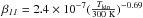 and k15 = 8.8 × 10⁻¹⁰cm3 s-1 are adopted from UMIST database (Woodall et al. 2007).
From Table 8, we found that the lower limit of ionization rate is ~10-7. This method makes some assumptions, e.g., CO depletion and fractional reaction are not considered, as discussed in Caselli et al. (1998), Lintott & Rawlings (2006), Miettinen et al. (2011). Nevertheless, these more precise, model-based estimations are consistent with those reported in HMSCs (e.g., Williams et al. 1998; Bergin et al. 1999; Chen et al. 2010; Miettinen et al. 2011) and the modeling result in Gerner et al. (2014). Moreover, the lower limit of ionization rate in our large-scale (~0.8 pc) HMSC envelopes is higher than the model-predicted values in the center of the low-mass prestellar objects (e.g., >10-9, Caselli et al. 2002c). This is reasonable because the cosmic ray ionization rates in the envelope of HMSCs are higher than in the inner region of their low-mass counterparts. It is also possible that these HMSCs are in a much more active environment than low-mass prestellar cores, and hence they are affected by much more radiation of any kind.
In addition, as mentioned in Sect. 3.2.2, H13CO+ is “deficient” in regions where 13CO is abundant in IRDC 18530. This can be explained by Eqs. (15)–(16), which show that the rate coefficient β11 is enhanced in this source.
5. Conclusions
To investigate the initial conditions of high-mass star formation, we carried out several observations with the SMA and IRAM 30 m. In this paper, we study the dynamic and chemical properties of four IRDCs (G28.34 S, IRDC 18530, IRDC 18306, and IRDC 18308), which exhibit strong (sub)mm continuum emission toward 70 μm extinction features. At different spatial resolutions and wavelengths, this small sample study of IRDCs illustrates that the cold (T< 15 K), dense (~105 cm-3) high-mass star-forming regions are not completely quiescent.
Our conclusions are as follows:
-
1.
At an angular resolution of2′′ (~104 AU at an average distance of 4 kpc), the 1.1 mm SMA observations resolve each source into several fragments. The average separation between the fragments is 0.07–0.24 pc, comparable to the Jeans length. However, the mass of each fragment is on average >10M⊙, exceeding the thermal Jeans mass of the entire clump by a factor of up to 30, indicating that thermal pressure alone does not dominate the fragmentation process.
-
2.
In the 8 GHz SMA observational band at 1.1 mm, higher-J transitions (including dense gas tracers such as H13CO+ (2 → 1)) are not detected, implying that our sources are in the cold and young evolutionary status when lines with Eu/kB> 20 K may not be excited. However, our line survey at 1 mm/3 mm shows a number of emissions from lower-J transitions. In particular, a >5σ rms detection of SiO (2 → 1) with broad line wings in G28.34 S may be the signature of a potential protostellar object, and the asymmetric HCO+ line profile in this source traces potential infall motion at a speed of ~ 0.84 km s-1.
-
3.
Linewidths of all the 30 m detected lines are on average 2–3 km s-1. Using the H13CO+ (1 → 0) line, we calculate the velocity dispersion components and the critical mass based on a non-thermal fragmentation scenario. Non-thermal motions can provide sufficient extra support to increase the scale of the fragmentation, making it possible to support fragments up to several hundreds of M⊙ against gravity. Alternative explanations may include magnetic fields and steep core density profiles. The mass of the well-aligned fragments in filament G28.34 S and IRDC 18308 is also in rough agreement with the scenario of “cylindrical fragmentation”.
-
4.
N2H+ (J = 1 → 0), C2H (N = 1 → 0), HCN (J = 1 → 0), and H13CN (J = 1 → 0) have multiplets in our 30 m data. Using a hyperfine multiplet fit program, we estimate their excitation temperature (on average 5–8 K) and conclude that they are subthermally excited. The excitation temperatures of the CO isotopologues suggest that the sources are in the very early cold phase (~10 K).
-
5.
Our large-scale high-mass clumps exhibit chemical features that are qualitatively similar to low-mass prestellar cores on small scales, including a large number of N-bearing species and the detection of carbon rings and molecular ions. Moreover, G28.34 S and IRDC 18308 show anti-correlated spatial distributions between N2H+/NH2D and CO on a scale of 0.5 pc. We calculate the molecular abundances, HCN/HNC ratio, CO depletion factor, and ionization fraction and find that G28.34 S is slightly more chemically evolved than the other sources in our sample.
-
6.
Large-scale line surveys measure the chemical features of the high-mass clumps hosting HMSCs, but are not sufficient to probe the chemical complexity of the fragments themselves. The above observations reveal non-thermal motions, which dominate the fragmentation process from the dark cloud to the high-mass cores. However, without line detection, we do not know the dynamics within these cores. Further studies are expected to uncover the chemical and dynamic features within the densest fragments of IRDCs.
The APEX Telescope Large Area Survey of the Galaxy (ATLASGAL) is a large area survey of the galaxy at 870 μm (Schuller et al. 2009).
IRDCs are classified as “active” if they host protostellar dominated cores and “quiescent” if they host prestellar dominated cores, depending on whether both 4.5 and 24 μm emission is detected (Chambers et al. 2009; Rathborne et al. 2010).
The MIR package was originally developed for the Owens Valley Radio Observatory, and is now adapted for the SMA, http://cfa-www.harvard.edu/~cqi/mircook.html
The SMA continuum peak of each source has some shift from its observational phase center. Therefore, we set the 30 m mapping center according to the SMA continuum peak and use Gildas software to “reproject” the SMA offset accordingly.
The “Weeds” is an extension of Gildas for line identification (Maret et al. 2011).
A compilation of the Jet Propulsion Laboratory (JPL, http://spec.jpl.nasa.gov, Pickett et al. 1998), Cologne Database for Molecular Spectroscopy (CDMS, http://www.astro.uni-koeln.de/cdms/catalog, Müller et al. 2005), and Lovas/NIST catalogues (Lovas 2004), http://www.splatalogue.net
The HFS fit and the Gaussian fit are both based on the Gildas software package, http://www.iram.fr/IRAMFR/GILDAS/doc/html/class- html/class.html
For HCN in IRDC18306, we image the F = 1 → 1 line. For the rest, we image the line with the strongest relative intensity (according to CDMS/JPL line intensity at 300 K, ℓ(300 K) in Table A.1).
The SiO (6 → 5) line has only 2.5σ detection in our SMA data.
We fit the 2D Gaussian structure with CASA, http://casa.nrao.edu
We assume that the local temperature in the cut is the same at different radii, so the flux intensity profile is the first-order estimate instead of the density profile in Wang et al. (2015).
Since both the small-scale fragments and large-scale filaments show asymmetric structures, the simplification 2D Gaussian fit cannot provide more precise estimation of the volume number density than the method we use here.
Since a 2D Gaussian is not suitable for modeling a filamentary structure, we use the same algorithm that measures the total flux per unit projection size to measure the linear masses in rectangles, which are centered on the mapping center of 30 m observations and individually have lengths that are one, two, or three times the local FWHM width, and then derive the mean.
Even if the velocity distribution of our source is biased by our field of view, rotation energy is in general not comparable to the gravitational energy (Goodman et al. 1993; Bihr et al. 2015).
Following the method in Mardones et al. (1997), we set the threshold of “significance” as 5 times the uncertainty of δVH13CO+.
A more precise approach is to use the non-LTE radiative transfer code RADEX. However, it does not significantly improve our results, when we do not know the source structure.
The molecular abundance estimated in our study is, on average, one magnitude lower than the IRDC large sample study by Gerner et al. (2014). However, if we assume a higher Tkin ~ 15 K (as in Gerner et al. 2014), the molecular abundances are comparable.
Acknowledgments
We would like to thank the SMA staff and IRAM 30 m staff for their helpful support during the reduction of the SMA data and the performance of the IRAM 30 m observations in service mode. We thank J. Pineda, Y. Wang, Z. Y. Zhang, and K. Wang for helpful discussions. We thank the anonymous reviewer for the constructive comments. This research made use of NASA’s Astrophysics Data System. The Submillimeter Array is a joint project between the Smithsonian Astrophysical Observatory and the Academia Sinica Institute of Astronomy and Astrophysics and is funded by the Smithsonian Institution and the Academia Sinica.
References
- Afonso, J. M., Yun, J. L., & Clemens, D. P. 1998, AJ, 115, 1111 [NASA ADS] [CrossRef] [Google Scholar]
- Aikawa, Y., Wakelam, V., Garrod, R. T., & Herbst, E. 2008, ApJ, 674, 984 [NASA ADS] [CrossRef] [Google Scholar]
- Bastien, P., Arcoragi, J.-P., Benz, W., Bonnell, I., & Martel, H. 1991, ApJ, 378, 255 [NASA ADS] [CrossRef] [Google Scholar]
- Bergin, E. A. 2003, in SFChem 2002: Chemistry as a Diagnostic of Star Formation, eds. C. L. Curry, & M. Fich (Ottawa: National Research Council Press), 63 [Google Scholar]
- Bergin, E. A., & Tafalla, M. 2007, ARA&A, 45, 339 [NASA ADS] [CrossRef] [Google Scholar]
- Bergin, E. A., Goldsmith, P. F., Snell, R. L., & Ungerechts, H. 1994, ApJ, 431, 674 [NASA ADS] [CrossRef] [Google Scholar]
- Bergin, E. A., Snell, R. L., & Goldsmith, P. F. 1996, ApJ, 460, 343 [NASA ADS] [CrossRef] [Google Scholar]
- Bergin, E. A., Plume, R., Williams, J. P., & Myers, P. C. 1999, ApJ, 512, 724 [NASA ADS] [CrossRef] [Google Scholar]
- Bergin, E. A., Alves, J., Huard, T., & Lada, C. J. 2002, ApJ, 570, L101 [NASA ADS] [CrossRef] [Google Scholar]
- Beuther, H., & Sridharan, T. K. 2007, ApJ, 668, 348 [NASA ADS] [CrossRef] [Google Scholar]
- Beuther, H., & Henning, T. 2009, A&A, 503, 859 [NASA ADS] [CrossRef] [EDP Sciences] [Google Scholar]
- Beuther, H., Schilke, P., Menten, K. M., et al. 2002, ApJ, 566, 945 [NASA ADS] [CrossRef] [Google Scholar]
- Beuther, H., Semenov, D., Henning, T., & Linz, H. 2008, ApJ, 675, L33 [NASA ADS] [CrossRef] [Google Scholar]
- Beuther, H., Zhang, Q., Bergin, E. A., & Sridharan, T. K. 2009, AJ, 137, 406 [NASA ADS] [CrossRef] [Google Scholar]
- Beuther, H., Henning, T., Linz, H., et al. 2010, A&A, 518, L78 [NASA ADS] [CrossRef] [EDP Sciences] [Google Scholar]
- Beuther, H., Kainulainen, J., Henning, T., Plume, R., & Heitsch, F. 2011, A&A, 533, A17 [NASA ADS] [CrossRef] [EDP Sciences] [Google Scholar]
- Beuther, H., Tackenberg, J., Linz, H., et al. 2012, A&A, 538, A11 [NASA ADS] [CrossRef] [EDP Sciences] [Google Scholar]
- Beuther, H., Linz, H., Tackenberg, J., et al. 2013, A&A, 553, A115 [NASA ADS] [CrossRef] [EDP Sciences] [Google Scholar]
- Beuther, H., Henning, T., Linz, H., et al. 2015, A&A, 581, A119 [NASA ADS] [CrossRef] [EDP Sciences] [Google Scholar]
- Bihr, S., Beuther, H., Linz, H., et al. 2015, A&A, 579, A51 [NASA ADS] [CrossRef] [EDP Sciences] [Google Scholar]
- Blake, G. A., Sutton, E. C., Masson, C. R., & Phillips, T. G. 1987, ApJ, 315, 621 [NASA ADS] [CrossRef] [Google Scholar]
- Bontemps, S., Motte, F., Csengeri, T., & Schneider, N. 2010, A&A, 524, A18 [NASA ADS] [CrossRef] [EDP Sciences] [Google Scholar]
- Bronfman, L., Nyman, L.-A., & May, J. 1996, A&AS, 115, 81 [NASA ADS] [Google Scholar]
- Butler, M. J., & Tan, J. C. 2009, ApJ, 696, 484 [NASA ADS] [CrossRef] [Google Scholar]
- Carey, S. J., Clark, F. O., Egan, M. P., et al. 1998, ApJ, 508, 721 [NASA ADS] [CrossRef] [Google Scholar]
- Caselli, P., Walmsley, C. M., Terzieva, R., & Herbst, E. 1998, ApJ, 499, 234 [NASA ADS] [CrossRef] [Google Scholar]
- Caselli, P., Walmsley, C. M., Tafalla, M., Dore, L., & Myers, P. C. 1999, ApJ, 523, L165 [NASA ADS] [CrossRef] [Google Scholar]
- Caselli, P., Benson, P. J., Myers, P. C., & Tafalla, M. 2002a, ApJ, 572, 238 [NASA ADS] [CrossRef] [Google Scholar]
- Caselli, P., Walmsley, C. M., Zucconi, A., et al. 2002b, ApJ, 565, 331 [NASA ADS] [CrossRef] [Google Scholar]
- Caselli, P., Walmsley, C. M., Zucconi, A., et al. 2002c, ApJ, 565, 344 [NASA ADS] [CrossRef] [Google Scholar]
- Chambers, E. T., Jackson, J. M., Rathborne, J. M., & Simon, R. 2009, ApJS, 181, 360 [NASA ADS] [CrossRef] [Google Scholar]
- Chandrasekhar, S., & Fermi, E. 1953, ApJ, 118, 116 [NASA ADS] [CrossRef] [MathSciNet] [Google Scholar]
- Chen, H.-R., Liu, S.-Y., Su, Y.-N., & Zhang, Q. 2010, ApJ, 713, L50 [NASA ADS] [CrossRef] [Google Scholar]
- Chin, Y.-N., Henkel, C., Whiteoak, J. B., Langer, N., & Churchwell, E. B. 1996, A&A, 305, 960 [NASA ADS] [Google Scholar]
- Chira, R.-A., Beuther, H., Linz, H., et al. 2013, A&A, 552, A40 [NASA ADS] [CrossRef] [EDP Sciences] [Google Scholar]
- Codella, C., Bachiller, R., Nisini, B., Saraceno, P., & Testi, L. 2001, A&A, 376, 271 [NASA ADS] [CrossRef] [EDP Sciences] [Google Scholar]
- Commerçon, B., Hennebelle, P., & Henning, T. 2011, ApJ, 742, L9 [NASA ADS] [CrossRef] [Google Scholar]
- Crapsi, A., Caselli, P., Walmsley, C. M., et al. 2005, ApJ, 619, 379 [Google Scholar]
- Csengeri, T., Bontemps, S., Schneider, N., Motte, F., & Dib, S. 2011, A&A, 527, A135 [NASA ADS] [CrossRef] [EDP Sciences] [Google Scholar]
- Devine, K. E., Chandler, C. J., Brogan, C., et al. 2011, ApJ, 733, 44 [NASA ADS] [CrossRef] [Google Scholar]
- Dobbs, C. L., Bonnell, I. A., & Clark, P. C. 2005, MNRAS, 360, 2 [NASA ADS] [CrossRef] [MathSciNet] [Google Scholar]
- Draine, B. T. 2011, Physics of the Interstellar and Intergalactic Medium (Princeton University Press) [Google Scholar]
- Feng, S., Beuther, H., Semenov, D., et al. 2016, A&A, in press, DOI: 10.1051/0004-6361/201424912 [Google Scholar]
- Fiege, J. D., & Pudritz, R. E. 2000, MNRAS, 311, 85 [NASA ADS] [CrossRef] [Google Scholar]
- Fischera, J., & Martin, P. G. 2012, A&A, 542, A77 [NASA ADS] [CrossRef] [EDP Sciences] [Google Scholar]
- Fontani, F., Caselli, P., Crapsi, A., et al. 2006, A&A, 460, 709 [NASA ADS] [CrossRef] [EDP Sciences] [Google Scholar]
- Fontani, F., Giannetti, A., Beltrán, M. T., et al. 2012, MNRAS, 423, 2342 [NASA ADS] [CrossRef] [Google Scholar]
- Fontani, F., Sakai, T., Furuya, K., et al. 2014, MNRAS, 440, 448 [NASA ADS] [CrossRef] [Google Scholar]
- Frerking, M. A., Langer, W. D., & Wilson, R. W. 1982, ApJ, 262, 590 [NASA ADS] [CrossRef] [Google Scholar]
- Fuller, G. A., Williams, S. J., & Sridharan, T. K. 2005, A&A, 442, 949 [NASA ADS] [CrossRef] [EDP Sciences] [Google Scholar]
- Garrod, R. T., Weaver, S. L. W., & Herbst, E. 2008, ApJ, 682, 283 [NASA ADS] [CrossRef] [Google Scholar]
- Gerner, T., Beuther, H., Semenov, D., et al. 2014, A&A, 563, A97 [NASA ADS] [CrossRef] [EDP Sciences] [Google Scholar]
- Giannetti, A., Wyrowski, F., Brand, J., et al. 2014, A&A, 570, A65 [NASA ADS] [CrossRef] [EDP Sciences] [Google Scholar]
- Girichidis, P., Federrath, C., Banerjee, R., & Klessen, R. S. 2011, MNRAS, 413, 2741 [NASA ADS] [CrossRef] [Google Scholar]
- Goldsmith, P. F., Irvine, W. M., Hjalmarson, A., & Ellder, J. 1986, ApJ, 310, 383 [NASA ADS] [CrossRef] [PubMed] [Google Scholar]
- Goodman, A. A., Benson, P. J., Fuller, G. A., & Myers, P. C. 1993, ApJ, 406, 528 [NASA ADS] [CrossRef] [Google Scholar]
- Helmich, F. P., & van Dishoeck, E. F. 1997, A&AS, 124, 205 [NASA ADS] [CrossRef] [EDP Sciences] [Google Scholar]
- Henning, T., Linz, H., Krause, O., et al. 2010, A&A, 518, L95 [NASA ADS] [CrossRef] [EDP Sciences] [Google Scholar]
- Hildebrand, R. H. 1983, QJRAS, 24, 267 [NASA ADS] [Google Scholar]
- Hirota, T., Yamamoto, S., Mikami, H., & Ohishi, M. 1998, ApJ, 503, 717 [NASA ADS] [CrossRef] [Google Scholar]
- Ho, P. T. P., Moran, J. M., & Lo, K. Y. 2004, ApJ, 616, L1 [NASA ADS] [CrossRef] [Google Scholar]
- Hofner, P., Wiesemeyer, H., & Henning, T. 2001, ApJ, 549, 425 [NASA ADS] [CrossRef] [Google Scholar]
- Horn, A., Møllendal, H., Sekiguchi, O., et al. 2004, ApJ, 611, 605 [NASA ADS] [CrossRef] [Google Scholar]
- Inutsuka, S.-I., & Miyama, S. M. 1992, ApJ, 388, 392 [NASA ADS] [CrossRef] [Google Scholar]
- Jackson, J. M., Finn, S. C., Chambers, E. T., Rathborne, J. M., & Simon, R. 2010, ApJ, 719, L185 [NASA ADS] [CrossRef] [Google Scholar]
- Jiménez-Serra, I., Martín-Pintado, J., Caselli, P., Viti, S., & Rodríguez-Franco, A. 2009, ApJ, 695, 149 [NASA ADS] [CrossRef] [Google Scholar]
- Jiménez-Serra, I., Caselli, P., Tan, J. C., et al. 2010, MNRAS, 406, 187 [NASA ADS] [CrossRef] [Google Scholar]
- Jin, M., Lee, J.-E., & Kim, K.-T. 2015, ApJS, 219, 2 [NASA ADS] [CrossRef] [Google Scholar]
- Jones, P. A., Burton, M. G., Cunningham, M. R., et al. 2008, MNRAS, 386, 117 [NASA ADS] [CrossRef] [Google Scholar]
- Jørgensen, J. K., Schöier, F. L., & van Dishoeck, E. F. 2004, A&A, 416, 603 [NASA ADS] [CrossRef] [EDP Sciences] [Google Scholar]
- Kainulainen, J., Ragan, S. E., Henning, T., & Stutz, A. 2013, A&A, 557, A120 [NASA ADS] [CrossRef] [EDP Sciences] [Google Scholar]
- Kirk, H., Johnstone, D., & Di Francesco, J. 2006, ApJ, 646, 1009 [NASA ADS] [CrossRef] [Google Scholar]
- Kirk, H., Klassen, M., Pudritz, R., & Pillsworth, S. 2015, ApJ, 802, 75 [NASA ADS] [CrossRef] [Google Scholar]
- Krumholz, M. R., & McKee, C. F. 2008, Nature, 451, 1082 [NASA ADS] [CrossRef] [PubMed] [Google Scholar]
- Lee, C. W., Myers, P. C., & Tafalla, M. 2001, ApJS, 136, 703 [NASA ADS] [CrossRef] [Google Scholar]
- Lintott, C. J., & Rawlings, J. M. C. 2006, A&A, 448, 425 [NASA ADS] [CrossRef] [EDP Sciences] [Google Scholar]
- Linz, H., Krause, O., Beuther, H., et al. 2010, A&A, 518, L123 [NASA ADS] [CrossRef] [EDP Sciences] [Google Scholar]
- Loughnane, R. M., Redman, M. P., Thompson, M. A., et al. 2012, MNRAS, 420, 1367 [NASA ADS] [CrossRef] [Google Scholar]
- Lovas, F. J. 2004, Phys. Chem. Ref., 33, 117 [Google Scholar]
- Mardones, D., Myers, P. C., Tafalla, M., et al. 1997, ApJ, 489, 719 [NASA ADS] [CrossRef] [Google Scholar]
- Maret, S., Hily-Blant, P., Pety, J., Bardeau, S., & Reynier, E. 2011, A&A, 526, A47 [NASA ADS] [CrossRef] [EDP Sciences] [Google Scholar]
- Matthews, H. E., & Irvine, W. M. 1985, ApJ, 298, L61 [NASA ADS] [CrossRef] [Google Scholar]
- Meier, D. S., & Turner, J. L. 2005, ApJ, 618, 259 [NASA ADS] [CrossRef] [Google Scholar]
- Miettinen, O., Harju, J., Haikala, L. K., Kainulainen, J., & Johansson, L. E. B. 2009, A&A, 500, 845 [NASA ADS] [CrossRef] [EDP Sciences] [Google Scholar]
- Miettinen, O., Hennemann, M., & Linz, H. 2011, A&A, 534, A134 [NASA ADS] [CrossRef] [EDP Sciences] [Google Scholar]
- Motte, F., Bontemps, S., Schilke, P., et al. 2007, A&A, 476, 1243 [NASA ADS] [CrossRef] [EDP Sciences] [Google Scholar]
- Müller, H. S. P., Schlöder, F., Stutzki, J., & Winnewisser, G. 2005, J. Mol. Struct., 742, 215 [NASA ADS] [CrossRef] [Google Scholar]
- Myers, P. C., Linke, R. A., & Benson, P. J. 1983, ApJ, 264, 517 [NASA ADS] [CrossRef] [Google Scholar]
- Myers, P. C., Mardones, D., Tafalla, M., Williams, J. P., & Wilner, D. J. 1996, ApJ, 465, L133 [NASA ADS] [CrossRef] [Google Scholar]
- Nagasawa, M. 1987, Prog. Theor. Phys., 77, 635 [NASA ADS] [CrossRef] [Google Scholar]
- Nguyen-Lu’o’ng, Q., Motte, F., Carlhoff, P., et al. 2013, ApJ, 775, 88 [NASA ADS] [CrossRef] [Google Scholar]
- Ohishi, M., Irvine, W. M., & Kaifu, N. 1992, in Astrochemistry of Cosmic Phenomena, ed. P. D. Singh, IAU Symp., 150, 171 [NASA ADS] [CrossRef] [Google Scholar]
- Ossenkopf, V., & Henning, T. 1994, A&A, 291, 943 [NASA ADS] [Google Scholar]
- Palau, A., Rizzo, J. R., Girart, J. M., & Henkel, C. 2014, ApJ, 784, L21 [Google Scholar]
- Palumbo, M. E., Geballe, T. R., & Tielens, A. G. G. M. 1997, ApJ, 479, 839 [NASA ADS] [CrossRef] [Google Scholar]
- Pickett, H. M., Poynter, R. L., Cohen, E. A., et al. 1998, J. Quant. Spectr. Rad. Transf., 60, 883 [NASA ADS] [CrossRef] [Google Scholar]
- Pillai, T., Wyrowski, F., Carey, S. J., & Menten, K. M. 2006, A&A, 450, 569 [NASA ADS] [CrossRef] [EDP Sciences] [Google Scholar]
- Pillai, T., Kauffmann, J., Wyrowski, F., et al. 2011, A&A, 530, A118 [NASA ADS] [CrossRef] [EDP Sciences] [Google Scholar]
- Pineda, J. E., Caselli, P., & Goodman, A. A. 2008, ApJ, 679, 481 [NASA ADS] [CrossRef] [Google Scholar]
- Pirogov, L., Zinchenko, I., Caselli, P., Johansson, L. E. B., & Myers, P. C. 2003, A&A, 405, 639 [NASA ADS] [CrossRef] [EDP Sciences] [Google Scholar]
- Qi, C., Kessler, J. E., Koerner, D. W., Sargent, A. I., & Blake, G. A. 2003, ApJ, 597, 986 [NASA ADS] [CrossRef] [Google Scholar]
- Ragan, S. E., Bergin, E. A., Plume, R., et al. 2006, ApJS, 166, 567 [NASA ADS] [CrossRef] [Google Scholar]
- Ragan, S. E., Bergin, E. A., & Gutermuth, R. A. 2009, ApJ, 698, 324 [NASA ADS] [CrossRef] [Google Scholar]
- Ragan, S. E., Bergin, E. A., & Wilner, D. 2011, ApJ, 736, 163 [NASA ADS] [CrossRef] [Google Scholar]
- Ragan, S., Henning, T., Krause, O., et al. 2012a, A&A, 547, A49 [NASA ADS] [CrossRef] [EDP Sciences] [Google Scholar]
- Ragan, S. E., Heitsch, F., Bergin, E. A., & Wilner, D. 2012b, ApJ, 746, 174 [NASA ADS] [CrossRef] [Google Scholar]
- Ragan, S. E., Henning, T., & Beuther, H. 2013, A&A, 559, A79 [NASA ADS] [CrossRef] [EDP Sciences] [Google Scholar]
- Rathborne, J. M., Jackson, J. M., & Simon, R. 2006, ApJ, 641, 389 [NASA ADS] [CrossRef] [Google Scholar]
- Rathborne, J. M., Jackson, J. M., Chambers, E. T., et al. 2010, ApJ, 715, 310 [NASA ADS] [CrossRef] [Google Scholar]
- Rawlings, J. M. C., Taylor, S. D., & Williams, D. A. 2000, MNRAS, 313, 461 [NASA ADS] [CrossRef] [Google Scholar]
- Rawlings, J. M. C., Redman, M. P., Keto, E., & Williams, D. A. 2004, MNRAS, 351, 1054 [NASA ADS] [CrossRef] [Google Scholar]
- Russeil, D., Zavagno, A., Motte, F., et al. 2010, A&A, 515, A55 [NASA ADS] [CrossRef] [EDP Sciences] [Google Scholar]
- Sakai, T., Sakai, N., Kamegai, K., et al. 2008, ApJ, 678, 1049 [NASA ADS] [CrossRef] [Google Scholar]
- Sanhueza, P., Jackson, J. M., Foster, J. B., et al. 2012, ApJ, 756, 60 [NASA ADS] [CrossRef] [Google Scholar]
- Sarrasin, E., Abdallah, D. B., Wernli, M., et al. 2010, MNRAS, 404, 518 [NASA ADS] [Google Scholar]
- Sault, R. J., Teuben, P. J., & Wright, M. C. H. 1995, in Astronomical Data Analysis Software and Systems IV, eds. R. A. Shaw, H. E. Payne, & J. J. E. Hayes, ASP Conf. Ser., 77, 433 [Google Scholar]
- Schilke, P., Walmsley, C. M., Pineau Des Forets, G., et al. 1992, A&A, 256, 595 [NASA ADS] [Google Scholar]
- Schuller, F., Menten, K. M., Contreras, Y., et al. 2009, A&A, 504, 415 [NASA ADS] [CrossRef] [EDP Sciences] [Google Scholar]
- Shirley, Y. L. 2015, PASP, 127, 299 [NASA ADS] [CrossRef] [Google Scholar]
- Sohn, J., Lee, C. W., Park, Y.-S., et al. 2007, ApJ, 664, 928 [NASA ADS] [CrossRef] [Google Scholar]
- Sridharan, T. K., Beuther, H., Saito, M., Wyrowski, F., & Schilke, P. 2005, ApJ, 634, L57 [NASA ADS] [CrossRef] [Google Scholar]
- Tackenberg, J., Beuther, H., Henning, T., et al. 2012, A&A, 540, A113 [NASA ADS] [CrossRef] [EDP Sciences] [Google Scholar]
- Tafalla, M., Mardones, D., Myers, P. C., et al. 1998, ApJ, 504, 900 [NASA ADS] [CrossRef] [Google Scholar]
- Tafalla, M., Myers, P. C., Caselli, P., Walmsley, C. M., & Comito, C. 2002, ApJ, 569, 815 [NASA ADS] [CrossRef] [Google Scholar]
- Tafalla, M., Santiago-García, J., Myers, P. C., et al. 2006, A&A, 455, 577 [NASA ADS] [CrossRef] [EDP Sciences] [Google Scholar]
- Teyssier, D., Hennebelle, P., & Pérault, M. 2002, A&A, 382, 624 [NASA ADS] [CrossRef] [EDP Sciences] [Google Scholar]
- Vasyunina, T., Linz, H., Henning, T., et al. 2009, A&A, 499, 149 [NASA ADS] [CrossRef] [EDP Sciences] [Google Scholar]
- Vasyunina, T., Linz, H., Henning, T., et al. 2011, A&A, 527, A88 [NASA ADS] [CrossRef] [EDP Sciences] [Google Scholar]
- Walawender, J., Bally, J., Kirk, H., & Johnstone, D. 2005, AJ, 130, 1795 [NASA ADS] [CrossRef] [Google Scholar]
- Wang, Y., Zhang, Q., Rathborne, J. M., Jackson, J., & Wu, Y. 2006, ApJ, 651, L125 [NASA ADS] [CrossRef] [Google Scholar]
- Wang, Y., Zhang, Q., Pillai, T., Wyrowski, F., & Wu, Y. 2008, ApJ, 672, L33 [NASA ADS] [CrossRef] [Google Scholar]
- Wang, K., Zhang, Q., Wu, Y., & Zhang, H. 2011, ApJ, 735, 64 [NASA ADS] [CrossRef] [Google Scholar]
- Wang, K., Zhang, Q., Testi, L., et al. 2014, MNRAS, 439, 3275 [NASA ADS] [CrossRef] [Google Scholar]
- Wang, K., Testi, L., Ginsburg, A., et al. 2015, MNRAS, 450, 4043 [NASA ADS] [CrossRef] [MathSciNet] [Google Scholar]
- Wienen, M., Wyrowski, F., Schuller, F., et al. 2012, A&A, 544, A146 [NASA ADS] [CrossRef] [EDP Sciences] [Google Scholar]
- Williams, J. P., Bergin, E. A., Caselli, P., Myers, P. C., & Plume, R. 1998, ApJ, 503, 689 [NASA ADS] [CrossRef] [Google Scholar]
- Wilson, T. L., & Rood, R. 1994, ARA&A, 32, 191 [NASA ADS] [CrossRef] [Google Scholar]
- Woodall, J., Agúndez, M., Markwick-Kemper, A. J., & Millar, T. J. 2007, A&A, 466, 1197 [NASA ADS] [CrossRef] [EDP Sciences] [Google Scholar]
- Wu, J., Evans, II, N. J., Shirley, Y. L., & Knez, C. 2010, ApJS, 188, 313 [NASA ADS] [CrossRef] [Google Scholar]
- Zhang, Q., & Wang, K. 2011, ApJ, 733, 26 [NASA ADS] [CrossRef] [Google Scholar]
- Zhang, Q., Wang, Y., Pillai, T., & Rathborne, J. 2009, ApJ, 696, 268 [NASA ADS] [CrossRef] [Google Scholar]
- Zhang, Q., Wang, K., Lu, X., & Jiménez-Serra, I. 2015, ApJ, 804, 141 [NASA ADS] [CrossRef] [Google Scholar]
- Zinchenko, I., Henkel, C., & Mao, R. Q. 2000, A&A, 361, 1079 [NASA ADS] [Google Scholar]
Appendix A: Molecular column density based on the HFS fit
Identified lines from the 30 m line survey in G28.34 S.
Linewidth, the intensity integrated over the dispersion of each line (subtable I), and the integrated optical depth over the velocity dispersion of the strongest line among multiplet (subtable II).
Average column densities and abundances for molecules with hyperfine multiplet lines in a square region from [20′′, 20′′] to [−20′′, −20′′] of four IRDCs observed by IRAM 30 m.
Average column densities and abundances for molecules without hyperfine multiplet lines in a square region from [20′′, 20′′] to [−20′′, −20′′] of four IRDCs observed by IRAM 30 m.
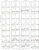 |
Fig. A.1 Line profiles of identified species toward each IRDC, ordered in groups as described in Sect. 3.2.2. The green line is from a single-Gaussian fit. “**” denotes a species with hyperfine multiplets whose HFS fits are plotted in Fig. 5. Profiles in blue denote the lines we detect from the “extra band” where the rms are higher than the others owing to less observation time. |
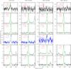 |
Fig. A.1 continued. |
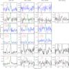 |
Fig. A.1 continued. Here a part of the multiplets of C2H is shown; the complete set of multiplets is in Fig. 5 |
The HFS method is based on the CLASS software package. In the fit model, the relative intensities with respect to the reference line (we set it as the strongest one) are converted from the ℓ(300 K) value in the Splatalogue database.
Four assumptions are made in the HFS fit for one species:
-
1.
All the components of the multiplet have the same excitationtemperature.
-
2.
The lines and their optical depths have Gaussian profiles.
-
3.
All the multiplets have the same linewidth.
-
4.
The multiplet components do not overlap.
One important parameter is the beam filling factor f. Although the distributions of most species are much more extended than the 30 m primary beam, the emission extents of some species (e.g., H13CN in IRDC 18306 and IRDC 18308) are smaller than the beam. To estimate the filling factor (on the first order), we define an equivalent angular diameter of the emission extent θmol as (Wu et al. 2010) 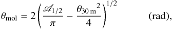 (A.1)where A1/2 is molecular extent within the contour of half maximum integrated intensity and θ30 m is the primary beam of 30 m at the molecular rest frequency.
With the beam filling factor 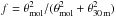 , background radiation temperature Tbg (assumed to be 2.7 K), and the intensity in units of temperature Jν(T) = (hν/kB)/ [exp(hν/kBT)−1], this method defines an effective intensity A as
 ![Mathematical equation: \appendix \setcounter{section}{1} \begin{equation} A=f\rm [{\it J_\nu}({\it T}_{ex})-{\it J_\nu}({\it T}_{bg})]~~~~~~~~~~~(K)\label{irdc:A} . \end{equation}](/articles/aa/full_html/2016/08/aa26864-15/aa26864-15-eq888.png) (A.2)The output parameters are Vlsr, the optical depth τ0, the linewidth Δυ, and the value of effective intensity affected by the line optical depth Aτ0 of the reference line. Therefore, with the light speed c, the Planck constant h, and a constant factor η = 2.7964 × 10⁻¹⁶ derived from Pickett et al. (1998), the excitation temperature of the multiplet Tex and the molecular column density NT,α at the frequency ν (in Hz) are given as
(A.2)The output parameters are Vlsr, the optical depth τ0, the linewidth Δυ, and the value of effective intensity affected by the line optical depth Aτ0 of the reference line. Therefore, with the light speed c, the Planck constant h, and a constant factor η = 2.7964 × 10⁻¹⁶ derived from Pickett et al. (1998), the excitation temperature of the multiplet Tex and the molecular column density NT,α at the frequency ν (in Hz) are given as ![Mathematical equation: \appendix \setcounter{section}{1} \begin{eqnarray} \label{irdc:hyper_tex} T_{\rm ex}&=& \frac{h\nu/k_{\rm B}}{\ln\left[\frac{h\nu/k_{\rm B}}{{\it A/f+J_\nu}(T_{\rm bg})}+1\right]}~~~~~~~~~~~({\rm K}) \\\label{irdc:hyper_NT} N_{T,\alpha}&=&\frac{8 \pi \nu}{ \ell(T_{\rm ex})\eta c^3} \tau_0 \Delta \upsilon~~~~~~~~~~~({\rm cm}^{-2}). \end{eqnarray}](/articles/aa/full_html/2016/08/aa26864-15/aa26864-15-eq896.png)
Appendix B: Opacities and excitation temperatures of CO isotopologue lines
13CO (2 → 1), C18O (2 → 1), and C17O (2 → 1) are all detected in our data. To estimate their excitation temperatures, we need to know their optical depths. Assuming that fractionation (isotopic exchange reaction) of 12C ⇔ 13C and of 17O ⇔ 16O ⇔ 18O are stable, we can estimate the optical depth at the line center of a given transition τα,0 by measuring the ratio between the main beam brightness temperature of the main line Tmb,α,0 and its isotopologue Tmb,β,0, (Myers et al. 1983): 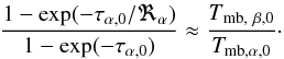 (B.1)Here ℜα is the intrinsic abundance of the main isotope (e.g., 12C) compared to its rare isotope (e.g., 13C) in the ISM (e.g., Wilson & Rood 1994; Chin et al. 1996).
Since the line profiles of CO isotopologues in our sample are contributions from various Galactic arms (Beuther & Sridharan 2007), we use a multi-Gaussian profile to fit their Tmb. Then, assuming that C17O (2 → 1) is optically thin and that all the lines are in LTE, we use Eq. (B.1) and the canonical ratio between isotopes (the following Eqs. (B.3)–(B.5), Frerking et al. 1982; Wilson & Rood 1994; Giannetti et al. 2014) to correct the optical depth of 13CO (2 → 1) and C18O (2 → 1). 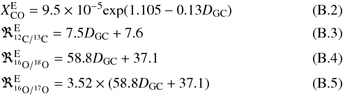 where DGC (kpc) is the galactic center distance, and
  is the canonical (undepleted) abundance of isotopologue α with respect to H2.
Subsequently, using Eq. (B.6), we estimate Tex of each CO isotopologue (see Table 7): ![Mathematical equation: \appendix \setcounter{section}{2} \begin{equation} T_{\rm ex}= \frac{h\nu_\alpha/k_{\rm B}}{\ln\left[\frac{h\nu_\alpha/k_{\rm B}}{{T_{\rm mb,\alpha,0}/(1-{\rm e}^{-\tau_\alpha})+J_\alpha}(T_{\rm bg})}+1\right]}~~~~~~~~~~~({\rm K}). \label{irdc:ratioab} \end{equation}](/articles/aa/full_html/2016/08/aa26864-15/aa26864-15-eq907.png) (B.6)
(B.6)
Appendix C: Molecular column densities for species without hyperfine multiplets
Consistent Tex of CO isotopologues (Table 7) indicates they are in LTE. Since most of the other lines without hyperfine multiples have low critical density (except for SiO (2 → 1)), we assume they are coupled with dust and thermalized at Tgas = Tdust = Tkin ~ Tex,CO. The column densities of these species can be derived as 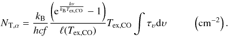 (C.1)Assuming that the observed emission homogeneously distributes in the primary beam of 30 m, the integration of measured main beam brightness temperature within the velocity range
  can be substituted for the last term in the above equation:
 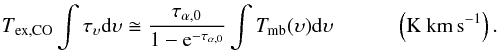 (C.2)(1) For species with neither a hyperfine multiplet nor a rare isotopologue, we assume they are optically thin, therefore,
  . (2) HCO+, HNC, and 13CO: 13CO (2 → 1) is optically thick in at least two of our sources when measured with C17O (2 → 1), and the other lines may have the same issue. As we have the rare isotopologues of HCO+ (1 → 0) and HNC (1 → 0) in our data, we use Eq. (B.1) to obtain their optical depths and correct their column densities by assuming that both H13CO+ (1 → 0) and HN13C (1 → 0) are optically thin.
In sources where the emission of species ≤3σ rms, we give their column density upper limit by assuming that f is unity.
All Tables
SMA observations toward four IRDCs: phase center of each source and the synthetic image quality at different configurations.
The parameters measured from SMA observations at 1.1 mm, including the coordinates, specific intensity at continuum peak, total flux density, and projected source size.
Parameters from 30 m and APEX observations and estimates based on two hypotheses of fragmentation (thermal Jeans fragmentation and turbulent Jeans fragmentation).
Tex derived from hyperfine fits to N2H+, C2H, HCN, and H13CN multiplets in four IRDCs.
CO depletion, HNC/HCN ratio, lower limit of ionization, and velocity asymmetric degree of H13CO+ in four IRDCs.
Linewidth, the intensity integrated over the dispersion of each line (subtable I), and the integrated optical depth over the velocity dispersion of the strongest line among multiplet (subtable II).
Average column densities and abundances for molecules with hyperfine multiplet lines in a square region from [20′′, 20′′] to [−20′′, −20′′] of four IRDCs observed by IRAM 30 m.
Average column densities and abundances for molecules without hyperfine multiplet lines in a square region from [20′′, 20′′] to [−20′′, −20′′] of four IRDCs observed by IRAM 30 m.
All Figures
|
Fig. 1 Compilation of the continuum data from 70 μm to 1.1 mm wavelength for G28.34 S, IRDC 18530, IRDC 18306, and IRDC 18308. Left column: graymaps of the dust emission observed by Herschel at 70 μm (Ragan et al. 2012a). The red contours show continuum emission observed by ATLASGAL at 870 μm (Schuller et al. 2009), starting from 10σ rms and continuing in 10σ rms steps. Middle and Right columns: black contours show continuum observed by SMA COMP configuration (middle) and COMP+EXT combination (right), overlaying the moment 0 colormaps of H13CO+(1 → 0) (integrated through its velocity dispersion) from IRAM 30 m observations. COMP contours start from 5σ rms and continue in 5σ rms steps, while COMP+EXT contours start from 3σ and continue in 3σ steps. 1σ rms of each source configuration is listed in Table 3. Cyan letters mark the fragments having >3σ rms continuum emission in both COMP and COMP+EXT maps. In each panel of the middle and right columns, the SMA synthesized beam is in the bottom left. The cyan circles show the primary beam of SMA at 1.1 mm, and the black dashed circles show the beam of 30 m at 3 mm. |
| In the text | |
|
Fig. 2 Averaged spectra from IRAM 30 m line survey at 3 mm/1 mm, which are extracted from a square region ([20′′, 20′′] to [−20′′, −20′′] offset) centered on the SMA continuum peak. The spectral resolution is 0.194 MHz (0.265 km s-1 at 1 mm and 0.641 km s-1 at 3 mm). All detected lines are labeled. The “extra band” is not shown here because of less integration time and thus there is a lower signal-to-noise ratio. |
| In the text | |
|
Fig. 3 Molecular line integrated intensity maps overlaid with the 870 μm continuum contours in G28.34 S, IRDC 18530, IRDC 18306, and IRDC 18308. The maps in each source are ordered in different groups according to line rest frequencies and the leading isotopes. Colormaps show the intensity integrations (K km s-1) over the velocity dispersion of each line. For the lines with <4σ detections, we only integrate a total of three channels around the system Vlsr at their rest frequencies. The purple contour in each panel indicates the area with integrated intensity >4σ rms. The black contour indicates the area within which integrated intensity is over the half maximum in the field of view. The white contours show the continuum emission from 870 μm ATLASGAL data, starting from 10σ and increasing by 10σ. |
| In the text | |
|
Fig. 3 continued. |
| In the text | |
|
Fig. 3 continued. |
| In the text | |
|
Fig. 3 continued. |
| In the text | |
|
Fig. 4 Asymmetric line profile of HCO+(1 → 0) compared to H13CO+(1 → 0) in G28.34 S, indicating infall motion with a speed of ~0.84 km s-1. |
| In the text | |
|
Fig. 5 Hyperfine multiplet fits (green lines) to the observed N2H+ (J = 1 → 0), C2H (N = 1 → 0), HCN (J = 1 → 0), and H13CN (J = 1 → 0) (black histograms) from each IRDC; the fit parameters are in the right upper corner. The transitions of multiplets are labeled in the panels of G28.34 S (with the strongest line in red). |
| In the text | |
|
Fig. 4 continued. |
| In the text | |
|
Fig. A.1 Line profiles of identified species toward each IRDC, ordered in groups as described in Sect. 3.2.2. The green line is from a single-Gaussian fit. “**” denotes a species with hyperfine multiplets whose HFS fits are plotted in Fig. 5. Profiles in blue denote the lines we detect from the “extra band” where the rms are higher than the others owing to less observation time. |
| In the text | |
|
Fig. A.1 continued. |
| In the text | |
|
Fig. A.1 continued. Here a part of the multiplets of C2H is shown; the complete set of multiplets is in Fig. 5 |
| In the text | |
Current usage metrics show cumulative count of Article Views (full-text article views including HTML views, PDF and ePub downloads, according to the available data) and Abstracts Views on Vision4Press platform.
Data correspond to usage on the plateform after 2015. The current usage metrics is available 48-96 hours after online publication and is updated daily on week days.
Initial download of the metrics may take a while.