| Issue |
A&A
Volume 592, August 2016
|
|
|---|---|---|
| Article Number | A48 | |
| Number of page(s) | 19 | |
| Section | Cosmology (including clusters of galaxies) | |
| DOI | https://doi.org/10.1051/0004-6361/201526479 | |
| Published online | 20 July 2016 | |
An alternative validation strategy for the Planck cluster catalogue and y-distortion maps⋆
1 Max Planck Institut für Astrophysik, Karl-Schwarzschild-Str. 1, 85741 Garching, Germany
e-mail: khatri@theory.tifr.res.in
2 Tata Institute of Fundamental Research, Homi Bhabha Road, 400005 Mumbai, India
Received: 6 May 2015
Accepted: 23 May 2016
We present an all-sky map of the y-type distortion calculated from the full mission Planck High Frequency Instrument (HFI) data using the recently proposed approach to component separation, which is based on parametric model fitting and model selection. This simple model-selection approach enables us to distinguish between carbon monoxide (CO) line emission and y-type distortion, something that is not possible using the internal linear combination based methods. We create a mask to cover the regions of significant CO emission relying on the information in the χ2 map that was obtained when fitting for the y-distortion and CO emission to the lowest four HFI channels. We revisit the second Planck cluster catalogue and try to quantify the quality of the cluster candidates in an approach that is similar in spirit to Aghanim et al. (2015, A&A, 580, A138). We find that at least 93% of the clusters in the cosmology sample are free of CO contamination. We also find that 59% of unconfirmed candidates may have significant contamination from molecular clouds. We agree with Planck Collaboration XXVII (2016, A&A, in press) on the worst offenders. We suggest an alternative validation strategy of measuring and subtracting the CO emission from the Planck cluster candidates using radio telescopes, thus improving the reliability of the catalogue. Our CO mask and annotations to the Planck cluster catalogue, identifying cluster candidates with possible CO contamination, are made publicly available.
Key words: cosmic background radiation / cosmology: observations / ISM: clouds / radio lines: ISM / methods: data analysis / galaxies: clusters: intracluster medium
The full Tables 1–3 are only available at the CDS via anonymous ftp to cdsarc.u-strasbg.fr (130.79.128.5) or via http://cdsarc.u-strasbg.fr/viz-bin/qcat?J/A+A/592/A48
© ESO, 2016
1. Introduction
The Planck experiment (Planck Collaboration I 2011), with its unprecedented sensitivity and multi-frequency full-sky coverage, has made it possible for the first time to create a full-sky map of the y-type distortion (Planck Collaboration XXI 2014; Planck Collaboration XXII 2016; Hill & Spergel 2014) and detect the y-type distortion in hundreds of known and newly discovered clusters (Planck Collaboration XXIX 2014; Planck Collaboration XXVII 2016). The y-distortion (Zeldovich & Sunyaev 1969) maps and cluster catalogues have been used to constrain cosmological parameters and cluster physics (Planck Collaboration XX 2014; Planck Collaboration Int. V 2013; Planck Collaboration Int. VIII 2013; Planck Collaboration Int. X 2013; Planck Collaboration Int. XI 2013; Hill & Spergel 2014; Planck Collaboration XXIV 2016; Hurier et al. 2015; Ruan et al. 2015). However about 27.2% of the cluster candidates in the second Planck catalogue are still unconfirmed. The traditional validation strategy for the cluster candidates relies on X-ray and optical observations (Planck Collaboration Int. IV 2013; Planck Collaboration XXIX 2016; Planck Collaboration Int. XXXVI 2016).
The Planck HFI channels, 100, 143, 217, and 353 GHz, which are most useful for the y-distortion studies also encompass the strong CO emission lines in three of the channels. The Galactic CO emission, with its non-trivial, non-monotonic spectrum, is therefore expected to be a non-negligible contaminant in these channels and hence in any y-distortion maps that are produced using these channels. It is more of a problem for the y-type distortion compared to the cosmic microwave background (CMB) temperature anisotropies because of the weakness of the y-distortion signal. The methods that have been employed so far to separate out the y-type distortion from Planck maps rely on internal linear combination (ILC) techniques (Hurier et al. 2013; Remazeilles et al. 2011; Planck Collaboration XXII 2016; Hill & Spergel 2014), which give the best fit estimates of the y-distortion on the sky, but cannot quantify the contamination from other components. An advantage of the ILC based component separation methods is that we do not need to know the emission spectrum of other components to separate out the component we are interested in. We follow a different approach, based on the recently developed linearized iterative least-squares (LIL; Khatri 2015) parametric model fitting and model selection algorithm. Our method requires a parametric model to be specified and therefore needs the spectral form of the other components. An advantage of the parametric model-fitting is that we get a quantitative estimate of how good the model fits the data in the residuals or χ2 of the fit, which can be used to accept or reject a given model of sky emission. We specifically use this method to select between CO emission and y-type distortion in every pixel on the sky, assuming that one or the other component dominates. Our test also gives an indication when both components may be present on the sky with neither component dominating, signifying for example, that a cluster may be present, but the y-type distortion signal estimate may be contaminated by the CO emission.
We apply our method to the Planck HFI data to construct CO emission and y-type distortion maps and use these maps together with the corresponding χ2 maps to construct a CO mask that specifies the minimum recommended area on the sky that should be masked for cosmological and y-distortion studies. We also revisit the Planck cluster catalogue and identify candidates which might in fact be molecular clouds or may have significant contamination from the CO emission from molecular clouds. This part of the paper is similar in spirit to the more sophisticated analysis based on neural networks of Aghanim et al. (2015), but uses a much simpler test based on the χ2 to select between two competing models and concentrates on differentiating the Galactic molecular clouds from clusters. Our analysis suggests an alternative strategy of “negative validation” using ground-based radio telescopes to look for the CO emission in candidates that are strongly indicated to be molecular clouds. In the direction of real clusters, where we identify significant CO contamination, radio telescopes can be used to measure and clean the CO emission from these clusters. This strategy may greatly help improve the reliability of the y-distortion signal in real clusters and of the cluster catalogue as a whole.
2. Construction of full sky map of y-type distortion from Planck data
Planck experiment has nine frequency channels covering the frequency range 30 GHz to 857 GHz. The angular resolutions of the lowest three LFI (low frequency instrument) channels at 30 GHz, 44 GHz, 70 GHz, are 32′,27′,13′, respectively (Planck Collaboration IV 2016). In addition, they have much higher noise compared to the High Frequency Instrument (HFI) channels and are therefore are not suitable for looking for weak and spatially concentrated signals such as y-type distortion. We therefore only use HFI channels in our study. The highest two HFI channels at 545 and 857 GHz are dominated by dust. We use a simple grey body spectrum with fixed temperature but varying spectral index to model dust. This is expected to be a good approximation in the Rayleigh-Jeans region where the spectral shape is not sensitive to the exact temperature but not accurate enough at 545 GHz and higher frequencies as we get closer to the peak of the grey body We therefore use the four frequencies channels at 100,143,217, and 353 GHz to construct a y-distortion map and use 545 GHz channel only to define a dust mask, i.e. a mask covering the regions of high dust emission above a certain threshold to select different fractions of the sky.
2.1. Contamination from y-type distortion in CO maps and vice versa
The frequency channels in the Planck experiment are rather broad and encompass many molecular lines, the most prominent of which are the  emission lines J = 1− → 0, J = 2− → 1, J = 3− → 2 which contribute to 100 GHz, 217 GHz, and 353 GHz channels (Planck Collaboration XIII 2014). We neglect the contributions from
  or other isotopologues. We would expect the CO emission from wide redshift bins to contribute to a given frequency channel and the same lines from different redshifts may contribute to different frequency channels. We use the 545 GHz map to mask strong point sources which should also mask most nearby strong sources of CO emission. However, except from the nearby galaxies, the CO emission contribution from external galaxies remains unresolved by Planck and would be part of the diffuse CO background which remains in our maps.
We want to mask the regions of high CO emission. The CO emission has a signal which changes in amplitude between different frequency channels in a non-monotonic way. Even though this variation is different from that of the y-type distortion, it is enough to present a serious contaminant as there are not enough frequency channels in Planck to simultaneously separate the CMB, y-type distortion, dust and CO emission. This is particularly important because the molecular clouds can present a morphology very similar to the galaxy clusters and there are regions on the sky with rather low dust emission but still non-negligible CO emission.
In principle, each Planck channel has many detectors with slightly different frequency response and it is possible to utilize the difference in transmission of lines in different detectors of the same channel to separate out the CO line emission. Planck collaboration uses this technique and the resulting maps are labeled as Type 1 maps using the MILCA component separation algorithm (Hurier et al. 2013; Planck Collaboration XIII 2014). These maps are however very noisy and not very useful except within a few degrees of the galactic plane. The most complete CO line survey is by Dame et al. (2001) who combined 37 individual surveys together to create a composite map of the galactic CO emission and the velocity integrated maps1. Unfortunately this map is also confined to mostly latitudes | b | ≲ 32° and does not extend to high latitudes which are of most interest for cosmology. There are many smaller surveys covering the galaxy away from the galactic plane in the northern as well as the southern galactic hemispheres (Magnani et al. 1985, 2000; Hartmann et al. 1998; Wilson et al. 2005) which have revealed the existence of molecular clouds at galactic latitudes up to | b | = 55°. With Planck of course we can detect the molecular clouds over the full sky. The difficulty, as we will see below, lies in separating the CO emission from the y-type distortion at high galactic latitudes and this is where our algorithm, to be discussed below, is efficient and most useful.
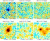 |
Fig. 1 Coma and Bullet clusters and SMC in Planck released CO Type 2 maps. Clusters show up as fake molecular clouds in J = 2− → 1 maps while strong clusters show up as negative sources in J = 1− → 0 maps. A 5 deg by 5 deg region around each source is shown. |
The second approach used by the Planck team is to use full channel maps and fit a parametric model to separate out the CO component and these are labeled Type 2 and Type 3 maps using the Commander-Ruler and Ruler (Eriksen et al. 2008; Planck Collaboration XII 2014) algorithms. Type 2 maps fit separately for the two lowest CO transitions while Type 3 maps assume a constant line ratio between the lines and fit for the common amplitude. The y-type distortion shows up as a negative source in Type 2 J = 1− → 0 maps since it contributes to the 100 GHz channel and as a positive source in J = 2− → 1 maps as this transition corresponds to 217 GHz channel where the y-distortion signal integrated over the band is positive. In principle therefore it is possible to use J = 1− → 0 line to distinguish between the negative y-distortion sources and the positive genuine molecular clouds. This map is however too noisy and misses weak CO sources, for example the small Magellanic clouds (SMC). A mask based on J = 2− → 1 maps will also mask all the clusters. To illustrate this we show the region around Coma and Bullet clusters and SMC in the publicly released Type 2 CO maps of Planck in Fig. 1. Type 3 maps are similar to the Type 2 J = 2− → 1 maps. There is of course negligible CO emission from the Coma and Bullet clusters and what we see in the CO maps is the y-distortion signal falsely identified as CO signal by the numerical fit to data. Similarly we expect that the CO emission would be falsely identified as y-distortion signal in the y-maps.
We derive the CO maps using the constant line ratios similar to the Planck type-3 maps which would then have similar contamination from clusters. We then follow a robust approach based on model selection to distinguish between the CO line emission and the y-type distortion.
2.2. Linearized iterative least-squares (LIL) parameter fitting
We want to fit the following parametric model to the four Planck frequency channels with frequencies 100,143,217, and 353 GHz at each pixel 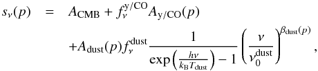 (1)where Ai are the amplitudes of the corresponding components, p is the pixel index in the map, βdust is the spectral index for the dust spectrum and
  . The factor of
  takes into account the colour correction for the dust spectrum (Planck Collaboration IX 2014) assuming a constant temperature, Tdust = 18.0 K. The factor of
  is the spectrum of the y-type distortion or the CO line emission, where we fit for either the CO line emission or the y-type distortion at a time.
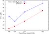 |
Fig. 2 CO and y spectrum as seen by different Planck channels after integrating over the detector response and conversion to thermodynamic CMB temperature units. |
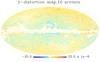 |
Fig. 3 Map of y-type distortion at 10′ resolution constructed from the lowest four Planck HFI channels. Approximately 14.2% of the area is masked. The prominent clusters can clearly be identified. Typical contamination from the foregrounds and noise is of order ~10-6. The ring like systematic features come from the Planck scanning strategy. |
Following (Planck Collaboration XIII 2014), we assume constant line ratios for the CO line contribution to the Planck HFI channels of 1:0.595:0.297 for (J = 1− → 0): (J = 2− → 1): (J = 3− → 2). The y-type spectrum at frequency ν is given by (Zeldovich & Sunyaev 1969) ![\begin{eqnarray} \Delta I_{\nu}=\frac{2 h\nu^3}{c^2}\frac{x e^x}{(e^x-1)^2}\left[x\left(\frac{e^x+1}{e^x-1}\right)-4\right], \end{eqnarray}](/articles/aa/full_html/2016/08/aa26479-15/aa26479-15-eq37.png) (2)where x = hν/ (kBTCMB), h is the Planck constant, kB is the Boltzmann constant, TCMB = 2.725 K is the CMB temperature and c is the speed of light. The factor includes conversion from the Rayleigh-Jeans (KRJ) temperature to thermodynamic CMB temperature units KCMB for dust and includes the conversion from KRJ km s-1 or dimensionless y amplitude for CO emission and y-type distortion respectively for different frequency channels (Planck Collaboration IX 2014) and are obtained by integrating the spectrum over the frequency response of the detectors. The CO spectrum and y-distortion spectrum as seen by Planck are compared in Fig. 2. An important difference between the two spectra is the rise in the CO spectrum at 100 GHz compared to the dip in the y-type spectrum. They are of course sufficiently similar that if we just try to extract one component by a linear combination of different channel maps, the two components will leak into each other. If only a CO component is present but we fit for a y component, we will expect a non-zero answer since the two components are not orthogonal. However if instead of doing a linear combination, we fit a parametric model, then these two spectra are sufficiently different that even though we would get a non-zero best fit answer for the wrong component, the fit would be much worse than expected from the available degrees of freedom, i.e. the residuals between the data and the model (χ2) would be very high. This is the key that enables us to separate the CO and the y-type components.
(2)where x = hν/ (kBTCMB), h is the Planck constant, kB is the Boltzmann constant, TCMB = 2.725 K is the CMB temperature and c is the speed of light. The factor includes conversion from the Rayleigh-Jeans (KRJ) temperature to thermodynamic CMB temperature units KCMB for dust and includes the conversion from KRJ km s-1 or dimensionless y amplitude for CO emission and y-type distortion respectively for different frequency channels (Planck Collaboration IX 2014) and are obtained by integrating the spectrum over the frequency response of the detectors. The CO spectrum and y-distortion spectrum as seen by Planck are compared in Fig. 2. An important difference between the two spectra is the rise in the CO spectrum at 100 GHz compared to the dip in the y-type spectrum. They are of course sufficiently similar that if we just try to extract one component by a linear combination of different channel maps, the two components will leak into each other. If only a CO component is present but we fit for a y component, we will expect a non-zero answer since the two components are not orthogonal. However if instead of doing a linear combination, we fit a parametric model, then these two spectra are sufficiently different that even though we would get a non-zero best fit answer for the wrong component, the fit would be much worse than expected from the available degrees of freedom, i.e. the residuals between the data and the model (χ2) would be very high. This is the key that enables us to separate the CO and the y-type components.
We use the recently developed LIL algorithm to fit for four parameters (three amplitudes and one dust spectral index) to four frequency channels at each pixel. We refer the reader to Khatri (2015) for the details of the parameter fitting algorithm. Here we just note a few important features of the algorithm. Since we are fitting four parameters to the four data points, it would appear that the degrees of freedom are zero. However in our algorithm the non-linear parameter is constrained to lie between values of 2 <βdust< 3 (Finkbeiner et al. 1999; Gold et al. 2011; Planck Collaboration XII 2014; Planck Collaboration XI 2014) and is not free to vary freely towards unphysical values where the true global minimum of the least squares problem may in fact lie. In particular in the regions of low dust contamination we do not expect to find the global or even local minimum of the χ2 in the βdust direction, and the value chosen for the βdust is just the best value within the constraints which often turns out to be one of the boundaries. Therefore the effective degree of freedom is usually close to one over most of the sky. Also the parameters are not arbitrary but belong to fixed models. So even while fitting four data points with four parameters, the χ2 would in general be ≫1 if the wrong model is being fit to the data. We rely on this feature to choose the correct model. Finally we want to rebeam all frequency channels to a common beam/angular resolution so that they are correctly weighted while parameter fitting. We use the channel beam window functions provided by the Planck collaboration as the beam profile of the respective channel maps (Planck Collaboration VII 2016). We then rebeam all the maps to a common 10′ FWHM Gaussian beam, which is close to the resolution of the lowest HFI frequency channel of 100 GHz and use the half-ring maps to estimate the noise in the rebeamed maps.
For both the y-type distortion and the CO emission we do nested model selection while fitting for the parameters as follows: we fit both a three parameter CMB+dust model and a four parameter CMB+dust+y/CO model. If an additional component corresponding to y or CO is present, we should get a big improvement in χ2 when we fit with the four parameters. The difference in χ2 for the three and four parameter models is again expected to be distributed as χ2 distribution for one degree of freedom (Stuart et al. 2004). If the y/CO components are absent we do not expect a big improvement in χ2. We can therefore set a threshold in Δχ2 improvement that we get when adding an extra component for accepting that component. If the improvement is smaller than the threshold we set the y or CO component to zero. For the CO component additionally we also put the additional constraint that it should be greater than zero. If during the fitting procedure the CO component falls below zero, we fix it to zero for the next few steps. A threshold of Δχ2 = 1.6,2.7,3.8 would correspond to the 20%, 10%, 5% probabilities respectively that we accept the y/CO component as present when it is in fact absent in a particular pixel. We use Δχ2 = 3.8 in the present paper. We have tested our results with different values of Δχ2, and for the construction of the CO mask and validation of the cluster catalogue, our results are not sensitive to the exact value of Δχ2.
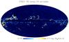 |
Fig. 4 Map of CO emission at 10′ resolution constructed from the lowest four Planck HFI channels. Approximately 10.2% of the area with extremely high dust emission and clusters are masked. |
The full sky y-distortion map computed for the Planck full mission data for Δχ2 = 3.8 is shown in Fig. 3 with the 14% of the area masked (y = 0 inside the masked area). We discuss the details of the mask computation in the next section. The official Planck full sky y-distortion maps (Planck Collaboration XXII 2016) computed using two algorithms based on the ILC technique, modified ILC algorithm (MILCA) Hurier et al. (2013) and Needlet ILC (NILC) Delabrouille et al. (2009), Remazeilles et al. (2011) are publicly available and we compare these with our map in Sect. 4. We also do an indirect comparison using the publicly available second Planck cluster catalogue. In particular, for the average y-type contribution from the Planck detected clusters we agree giving for the clean cluster sample (see below) an average ⟨ y ⟩ ≈ 4 × 10⁻⁸ (Khatri & Sunyaev 2015).
We also show in Fig. 4 our CO emission map. We have masked extremely high dust emission regions as well as the regions where our algorithm prefers a y-type distortion over the CO emission, i.e. the clusters. The algorithm used to create this y+dust mask is similar to the one used for the CO mask described below.
3. Model selection between CO and y-distortion, construction of CO mask and validation on real sky
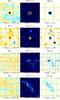 |
Fig. 5 Some external galaxies with different strengths and morphology in CO emission in our y-distortion and CO maps and difference in χ2 between the two model fits. A negative value implies that CO model is favored over the y-distortion. A negative y-distortion source near M51 is a radio point source. Galactic coordinates are shown. |
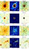 |
Fig. 6 Same as Fig. 5 but for the well known galaxy clusters. The |
The validation of our algorithm with the full focal plane (FFP6; Delabrouille et al. 2013) simulations was already performed in Khatri (2015) for the CO signal where we also compared our CO maps on the real sky with those released by the Planck collaboration and found good agreement. It was shown there that our algorithm recovers quite well the morphology of the CO emission. In this section we take a different approach of validating our algorithm as well as the model selection idea on the real sky using the known extragalactic sources of CO emission and clusters of galaxies. This is very important for us since the FFP6 simulations are based on the Dame et al. map (Dame et al. 2001) which as mentioned above does not cover high galactic latitudes where we want to do cosmological analysis. Note that this is the second level of model selection that we would perform now, in addition to the nested model selection already mentioned in the previous section. We now want to compare two models, CMB+dust+y and CMB+dust+CO, each with the same number of parameters. It is possible to use an information criterion to select between the models by looking at the difference  . Different information criterions differ mostly in how they penalize the new parameters (Stuart et al. 2004). Since the number of parameters and degrees of freedom for our two models are same, the different information criterions such as Akaike information criterion (Akaike 1974), Bayesian information criterion (Schwarz 1978) and Hannan-Quinn information criterion (Hannan & Quinn 1979) are equivalent for us. We use the CO and y distortion maps created with the nested model selection threshold of Δχ2 = 3.8 as discussed in the previous section.
We show in Fig. 5 our CO map, y map and 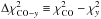 map several external galaxies. The M82 (Cigar galaxy) and M51 (Whirlpool galaxy) are unresolved strong sources of CO emission and are clearly identified as such in the
  map which takes large negative values. SMC is a resolved source with varying surface brightness across it. The morphology of our signal is in agreement with the that obtained from the dedicated CO (J = 1− → 0) line observations done with the NANTEN millimeter-wave telescope (Mizuno et al. 2001). Even a weak but large source as Andromeda (M31) is clearly identified as a CO source and the outer spiral arm which has the strongest CO emission can clearly be distinguished in the CO and χ2 maps. This ring like morphology of the CO emission in Andromeda agrees with the CO (J = 1− → 0) observations of Nieten et al. (2006) with the IRAM 30-m telescope. We have also detected the Antennae galaxies and M101 or Pinwheel galaxies in our CO maps as weak (as far as signal in Planck is concerned) sources of CO emission. We of course also detect the large Magellanic cloud (LMC) as a strong source of CO emission with morphology that again agrees with the dedicated observations from the Magellanic Mopra assessment (MAGMA) survey (Wong et al. 2011). The LMC can be clearly identified in our CO mask below (Fig. 7). We note that all these galaxies show significant y-distortion signal which is of course the CO emission contamination. Our χ2 test identifies the signal as CO emission in all the cases. Thus our algorithm can cleanly identify and mask out the sources of CO emission.
We show in Fig. 6 the maps for some of the known clusters. In this case the takes on average large positive values at the position of clusters signifying that the y-distortion model is preferred over the CO emission model. There is a bright radio source in the centre of Virgo cluster which shows up as negative y-distortion source. We discuss the handling of these sources also below when we create the CO mask.
The comparison of Figs. 5 and 6 shows that we can cleanly distinguish between CO emission and y-type distortion using the map and create a CO mask for y-distortion studies and vice versa. We use the following algorithm to create the mask.
-
1.
We first mask all pixels for which
 and also those pixels for which χ2 for the y-map is
  i.e. the y-distortion model was a very bad fit even without comparing with the CO map.
 -
2.
We then unmask all the pixels which were just masked as a result of statistical fluctuation by filling holes (masked regions) in the mask with size smaller than 50 pixels (in the HEALPix (Górski et al. 2005) nside = 2048 resolution maps) i.e. a region to be masked must have at least 50 pixels. This makes sure that only genuine CO regions are masked.
-
3.
We also want to mask point sources which may be smaller than 50 pixels in size. For this we repeat the first step with higher threshold
 . In addition we also mask pixels with large negative values of y-type distortion y< −50, and pixels with negative values and high χ2,
  . We then fill holes in the mask with a lower threshold of 12 pixels.
 -
4.
Finally we increase the mask by three pixels around the point sources and by five pixels everywhere else.
The above threshold were chosen so that we mask the known CO sources such as those shown in Fig. 5 while preserving even weak (in y-distortion) known clusters. There is a trade-off here: by being aggressive we can mask even the weak CO sources at the expense of deleting some weak clusters. By being conservative we can keep even the weak y-distortion signals at the expense of some contamination from the weak CO sources. Our thresholds are conservative and mask sources such as M51, M82, and SMC but do not mask Andromeda, the latter gives very weak contamination to the y-distortion map as shown in Fig. 5. We augment our mask slightly to mask regions with very high dust contamination using the 545 GHz channel. Our final mask covers 14.16% of sky leaving 85.84% of the sky unmasked. This is our minimal recommended mask that should be included in all studies of y-distortion in Planck data and is shown in Fig. 7. In practice we would further augment this mask using 545 GHz channel to get cleaner and cleaner parts of the sky to test the robustness of our results to contamination by dust. Our mask is available online2.
We show in Fig. 8 the χ2 distribution for pixels when fitting a y-distortion signal and a CO signal inside and outside our minimal 86% sky fraction mask (with the nested model selection turned off, Δχ2 = 0). As expected the χ2 distribution outside the mask is close to the χ2 distribution for one degree of freedom, also shown in the plot, signifying that our model is a good fit. The χ2 distribution is also slightly better (lower χ2 values) for a y distortion fit outside the mask compared to the CO spectrum. Inside the mask, the χ2 is slightly smaller for the model with CO, as expected. Note that for our model selection approach, only the difference in χ2 is important. Therefore, even though from the χ2 plot we see that inside the mask our model is not a good fit because the foregrounds become too complicated for our simple model, which ignores in particular the synchrotron component and fixes the CO spectrum, it still tells us that a y-distortion signal is a worse fit compared to the CO.
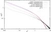 |
Fig. 8 χ2 distribution for the parameter fits by LIL for the y-distortion model and CO model compared with the χ2 distribution for one degree of freedom. |
4. Comparison with the MILCA/NILC y-maps
Planck collaboration has released two y-distortion maps computed using the ILC methods. The MILCA algorithm uses the HFI from 100 GHz to 545 GHz, and the 857 GHz channel on large angular scales. The NILC algorithm in addition also uses the LFI data on large angular scales, ℓ< 300Planck Collaboration XXII (2016). Both algorithms filter the maps with harmonic space window functions, apply ILC, and recombine the resulting y maps in ℓ windows to form the final y map. The main difference between the two algorithms is the bandpass window functions which for NILC correspond to the Needlet decomposition. The main advantage of performing an ILC is that we do not need to specify a model for the contamination. In particular the MILCA and NILC both remove a combination of the dust and CO foregrounds. This is the main difference from LIL where we explicitly remove the dust component but not the CO component. The LIL maps are therefore expected to have slightly higher level of CO contamination, which should not be a problem since the CO signal presents non-negligible contamination in only a small fraction of the sky which we mask. Note that since we explicitly take out the dust contamination modeled by a grey body spectrum, any other source of contamination with similar spectrum, such as the cosmic infrared background (CIB), is automatically fitted out by LIL. In this section we use the LIL y-map with Δχ2 = 0, i.e. with nested model selection turned off and y-type component included in all pixels.
Even though NILC and MILCA use higher number of channels, it is not enough to remove all CO and dust contamination. This is because some of the additional information coming from the 545 GHz channel is offset by the additional complexity of modeling the dust emission over a wider frequency range. We compare the three nearby galaxies, M31, M33, and M82 in Fig. 9, in NILC, MILCA, and LIL y-maps. These external galaxies, with known dust and CO emission morphologies, are good realistic test cases to study the extent of residual contamination in the y-maps. The contamination in the LIL map is correlated with the CO emission from these galaxies, as expected, and shows up in bright clumps in the spiral arms. For MILCA and NILC maps, the contamination has contribution from both residual dust and CO and is therefore more diffuse and is negative as well as positive. The contamination is slightly less in the NILC maps compared to the MILCA maps. We also show Coma cluster in the three y-maps in the last panel of Fig. 9 and the cluster y signal agrees between the two maps. The comparison of these external galaxies therefore reveals the complementarity of the parameter fitting LIL approach vs ILC approach.
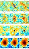 |
Fig. 9 Some external galaxies with different strengths and morphology in CO and dust emission are compared for different component separation methods. From top to bottom the galaxies shown are M31, M33, and M82. The last row shows the Coma cluster. |
We should clarify here that the main goal of our new method is not to produce a better y-map or to exactly reproduce the results of the Planck collaboration. Our main goal is to identify the regions of the sky with significant CO contamination. This is a worthwhile goal, since the CO contamination is a rare signal on the sky, just like the y-distortion signal. Since it occupies a small fraction of the sky area, it is possible to use targeted radio observations from ground to measure and remove the CO lines from the Planck maps. On these CO-free maps we can then apply the ILC/LIL methods to produce much cleaner and accurate y-distortion maps, since the ILC/LIL will now have less components to contend with. As we saw in the previous section, the χ2 based model selection, a standard statistics method Stuart et al. (2004), performs quite well in this regard.
We show in Fig. 10 the comparison of the 1d probability distribution functions (PDF), p(y), for the three maps for 51% of the sky utilizing the mask described in the previous section and augmenting it with a galactic dust mask constructed from the Planck 545 GHz map3. The tails at high values of y, contributed mostly by the already detected clusters of galaxies, agree for all maps. We also show the noise PDFs for LIL and NILC maps calculated from the half ring half difference (HRHD) maps. The MILCA noise is similar to NILC and both have smaller noise compared to the LIL maps. An important difference between NILC/MILCA and LIL is seen near the peak. The NILC/MILCA PDF is symmetric around the peak a result of explicitly removing the monopole in their component separation algorithms. In the LIL method we do not subtract the monopole and the PDF is skewed at small y as predicted Rubiño-Martín & Sunyaev (2003). This is apparent when we compare the y PDF with the noise PDF, the later being a symmetric Gaussian. This skewness is expected if we have unresolved y signal contributed by weak sources such as filaments and groups of galaxies. This is apparent in Fig. 11 where we masked 0.75° radius regions around all clusters and cluster candidates from the second Planck cluster catalogue Planck Collaboration XXVII (2016), with slightly bigger masks of 1.5° for sources with S/N> 30 and 4.5° for Perseus and Virgo.
It is also interesting to compare the performance of our masks with the galactic and point source masks released by the Planck collaboration with the y-distortion maps. We show our mask with 61% unmasked sky fraction, Planck collaboration galactic mask with 58% sky fraction and with the point source mask added to this mask yielding 49% sky fraction respectively in Figs. 12–14.
Our mask is not much more complicated than the Planck galactic mask but selectively masks out the point sources and molecular clouds which contaminate the y-distortion map. We plot the PDFs for LIL 61% and 51% masks as well as for the two Planck masks including and excluding the point source mask (labeled “plck”) for LIL and NILC y-maps in Figs. 15 and 16 respectively. For NILC PDF, we see that there are some peaks in the positive tail when using the Planck galactic mask which are not present in the LIL mask and are because of the molecular cloud contamination. The contamination in the negative tail is also significantly less for the LIL mask. The negative tail as well as the contamination in the positive tail is further reduced when we add the Planck point source mask. The difference between the Planck galactic mask and LIL mask is much greater for the LIL y-map because of the molecular cloud regions not covered by the galactic mask. The point source mask is however very dense and complicated and may also be masking significant genuine y-distortion signal Planck Collaboration XXII (2016). Our simple mask based on the model selection approach provides a good compromise between the two extremes of only using the Planck galactic masks and Planck galactic +point source masks. The LIL mask significantly reduces the contamination compared to the Planck galactic mask but without the overly complicated structure and complements the masks provided by the Planck collaboration.
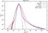 |
Fig. 10 1d PDF for NILC, MILCA, and LIL y-maps for the same mask with 51% sky. |
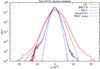 |
Fig. 11 1d PDF for NILC, MILCA, and LIL y-maps for the same mask with 51% sky and in addition with all the clusters from the second Planck cluster catalogue masked. |
 |
Fig. 12 Our mask with 61% sky fraction calculated using the model selection based approach described in the previous section. |
 |
Fig. 13 Galactic mask released by the Planck collaboration with the y-distortion maps with 58% unmasked fraction. |
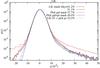 |
Fig. 15 Comparison of different masks for the LIL y-map. |
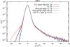 |
Fig. 16 Comparison of different masks for the NILC y-map. |
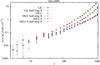 |
Fig. 17 Comparison of angular power spectra of LIL, MILCA, and NILC y-maps for 60% sky fraction mask. |
Finally we compare the angular power spectra of NILC, MILCA, and LIL maps in Fig. 17. We show the power spectra for the full mission maps, which includes noise, and the cross-spectra of the half-ring maps in which the noise is canceled. All power spectra are calculated with the publicly available PolSpice code Szapudi et al. (2001), Chon et al. (2004) and the effect of the mask Hivon et al. (2002) as well as the 10′ beam has been deconvolved. PolSpice also calculates the covariance matrix Efstathiou (2004), Challinor & Chon (2005), Tristram et al. (2005) which we have used to calculate the error bars for the ℓ bins. For the full mission map, we see the difference between the NILC/MILCA and LIL maps is because of the higher noise. All power spectra agree when the noise power is taken out in the half-ring cross spectra (labeled with half-ring-X suffix). Note that since the ILC algorithms are applied in small patches on the sky, the large scale modes, ℓ ≲ 10, would be influenced by the details of implementation, e.g. if monopole is subtracted in each patch. A LIL mask with 60% sky fraction (which is a smoother version of our 61% mask created using the 545 GHz channel map smoothed with 15° FWHM beam combined with the minimal 86% CO mask) and apodized with a Gaussian in pixel space was used. We apodized by replacing the 1s in the mask by ![\hbox{$1-\exp\left[-9\theta^2/(2\theta_{\rm ap}^2)\right]$}](/articles/aa/full_html/2016/08/aa26479-15/aa26479-15-eq82.png) , with θap = 60′ except for small point source like regions in the mask where we used θap = 30′ and θ is the distance from the mask edge.
, with θap = 60′ except for small point source like regions in the mask where we used θap = 30′ and θ is the distance from the mask edge.
5. Implications for the Planck cluster catalogue
Planck collaboration has released the second cluster catalogue (Planck Collaboration XXVII 2016) and we can do additional validation of our algorithm with this catalogue. Throughout this paper we use the second Planck catalogue. In particular we can check that the confirmed clusters fall outside our mask. We can also validate the Planck cluster catalogue using our results. In particular any unconfirmed candidates in the catalogue which fall inside our mask are likely to be molecular clouds rather than clusters.
Highest S/N noise clusters in the Planck catalogue.
We were however very conservative in creating our mask and we expect several weak molecular clouds to remain outside the mask. Instead of checking whether particular clusters fall inside or outside our mask we follow a different approach as follows. Since we have positions of cluster candidates in the catalogue, we can go to the position of each cluster and use our map to classify it as a cluster or a molecular cloud. The algorithm we use is the following:
-
1.
We sum the χ2 weighted by the square of signal in each pixel for all pixels within 5′ radius of each source in the catalogue and divide by the square of the maximum signal. We do this for both the CO maps and the y-maps to get the biased sum of squares
 and
and  for each source. This way we give more weight to the pixels at the centre of the source where we expect highest S/N and less weight to more numerous but low S/N pixels on the outskirts.
 -
2.
Since we used model selection with Δχ2 = 3.8 threshold while making the CO and y maps, for the weak sources there will be many pixels for which the CO or y amplitude is zero. We penalize these pixels by increasing the ∑ χ2, ∑ χ2− → ∑ χ2 + 4.0 for every zero pixel which is surrounded by non-zero pixels. This leaves out pixels which are zero and also surrounded by zero pixels. We penalize the map with smaller number of zero pixels by adding additional penalty to the corresponding χ2 of 4ΔN, where ΔN is the difference in zero pixels in the two maps which are also surrounded by zero pixels.
-
3.
If the final difference
 , we classify the source as cluster and add the annotation CLG to the table, if Δ( ∑ χ2)CO−y ≤ −10.0 we classify it as a molecular cloud with annotation MOC.
 -
4.
For a smaller threshold difference in Δ( ∑ χ2)CO−y of 5, we classify the cluster as pCLG or pMOC, with p signifying the lower significance of classification. Also if one of the maps has number of non-zero pixels less than 15, we use the annotation pCLG or pMOC even if the | Δ( ∑ χ2)CO−y | > 10.0.
-
5.
In the later case for the ∑ χ2 of the map with higher number of non-zero pixels N, if 1.6N< ∑ χ2 we classify the source as IND. If the difference Δ( ∑ χ2)CO−y is below the threshold we classify the source as IND or indeterminable by our algorithm. If both maps have non-zero pixels less than 15 we classify the source as IND.
This mostly heuristic algorithm works quite well in practice and we verified it by looking at the confirmed sources. There is in general a big difference in χ2 for strong sources unambiguously determining whether a source is a cluster or a molecular cloud. The classification we get is not very sensitive to small changes in the thresholds. Our full annotated Planck cluster catalogue is available online4. Note that we retain all entries from the Planck official catalogue and just add additional column with our annotation. We reproduce the top 10 highest signal to noise clusters from the catalogue in Table 1 and top highest signal to noise sources as well as 10 lowest signal to noise sources but with S/N> 6 that we have classified as molecular clouds in 2.
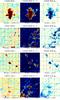 |
Fig. 18 Some of the candidates from Table 2 identified by our algorithm as molecular clouds or having significant contamination from the molecular clouds. |
It may seem surprising that quite a few confirmed clusters are identified as molecular clouds and this needs some explanation. First we note that the unconfirmed clusters have extremely high Δ( ∑ χ2)CO−y values and it would be very surprising if they turned out to be actual clusters. We show in Fig. 18 some sources from Table 2 with different Planck validation flags. The first source is an unconfirmed candidate that is almost surely a molecular cloud according to our analysis. This is also obvious visually in Fig. 18. The second row in Fig. 18 requires more attention. The source is located at the centre of the frame and is at the edge of a large molecular cloud. There is a confirmed X-ray cluster in the MCXC catalogue (meta-catalogue of X-ray detected clusters of galaxies, Piffaretti et al. 2011) at this position and our χ2 map shows a few pixels where a cluster is preferred over molecular cloud. However there is still significant CO emission from the foreground molecular cloud which seems to dominate over the y-signal and we expect that the amplitude of the distortion signal in the y-map to be unreliable. This interpretation is also confirmed by looking at the individual frequency maps centred at the same location in Fig. 19.
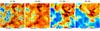 |
Fig. 19 Original Planck full channel maps smoothed to 10′ resolution at the location of the second source in Fig. 18 confirm the presence of molecular clouds in the foreground. Note that the scales in the last two maps are strictly positive. |
The third source in Fig. 18 was confirmed by arc-minute micro-Kelvin interferometer (AMI; Perrott et al. 2015) which operates at very low frequency of 15 GHz and may have contamination from the synchrotron emission from the molecular clouds. Our χ2 test shows that there is a molecular cloud clump at this location. The last row in Fig. 18 shows a source with low quoted S/N of ≈6 in the Planck catalogue which has Planck validation flag of 20 implying that it was present in the 2013 Planck catalogue (Planck Collaboration XXIX 2014) where it is listed as confirmed but there is no redshift information. Even if there is a cluster behind the molecular cloud, our analysis shows significant CO contamination to the y-signal.
In top panel in Fig. 20 we show the HI column density maps calculated by combining the Leiden/Dwingeloo survey data (Hartmann et al. 1996; Hartmann & Burton 1997) and the composite HI column density map of Dickey & Lockman (1990) and publicly available5 for the same sources as Fig. 18. In the bottom panel the Planck 857 data for the respective sources is shown. For the first source, the location of the cluster candidate coincides with region of low HI column density surrounded by high HI column density. The dust emission in the 857 GHz channel is also higher in the location of the source than in the surroundings. This is the signature that we would expect from a molecular cloud surrounded by an envelop of atomic HI gas. For the second source the situation is similar but not as clearly visible because both the dust emission and HI column density are higher and we are probably at the edge of a bigger molecular cloud. In the third and fourth source again there is agreement with the signature of the presence of a molecular cloud. The external HI column density data combined with Planck 857 GHz data therefore gives us confidence in our interpretation of these sources as molecular cloud candidates.
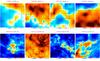 |
Fig. 20 HI column density and Planck 857 GHz emission for the sources shown in Fig. 18. The scale of all figures is same as the respective figures in Fig. 18 with the cluster candidates from the Planck catalogue at the centre of the frame. |
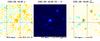 |
Fig. 21 One low S/N case where our test becomes unreliable visually however this preference towards it being a cluster can be inferred. |
Finally in Fig. 21 we show a marginal case of a low S/N source, the last entry in Table 2 where there is a confirmed x-ray cluster but the S/N is too low for a reliable distinction using our test. This is mostly because of the small angular size of the source resulting in most pixels in the 5′ radius having a zero signal so that our algorithm for summing up the χ2 is not optimal. However visual inspection shows that most pixels favor y-distortion over the CO contamination. Most of such sources would show up in our annotation with weaker validation code pMOC or pCLG.
To summarize, out of a total of 1653 sources in the Planck catalogue, we identify 395 molecular cloud candidates with annotation “MOC” and 97 molecular candidates with lower significance annotation “pMOC”. There are 450 unconfirmed clusters with Planck validation flag “− 1”, of which we classify 232 or 52% cluster candidates as “MOC”, and 35 candidates as “pMOC”. Therefore almost 59% of all the sources we identify as “MOC” are unconfirmed candidates.
The number of clusters above the threshold used by the Planck collaboration for cosmology sample, S/N> 6, is 693. Out of these 507 clusters have the cosmology flag set to “T”. From this cosmology sample we identify only 19 clusters as “MOC” and 18 clusters as “pMOC”. Of the remaining 186 clusters with S/N> 6, we identify 111 sources as “MOC” and 17 sources as “pMOC”. We thus confirm that the cosmology sample is much cleaner and reliable compared to the full cluster catalogue and we should expect significant contamination from the molecular clouds in the rest of the catalogue. We show in Fig. 22 the position of the 130 cluster candidates identified by us as strongly as molecular clouds with annotation “MOC” (white triangles) together with 528 sources which are identified by us as clusters or are undetermined by our algorithm with our annotations “CLG”, “pCLG” or “IND” (orange circles).
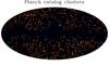 |
Fig. 22 Position on the sky in galactic coordinates of 528 sources from the Planck catalogue identified by us as likely to be clusters or indeterminable (orange circles) and 130 sources strongly likely to be molecular clouds (white triangles). |
5.1. Comparison with neural network based approach
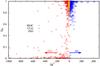 |
Fig. 23 Comparison of the two quality measures: our model selection based Δ( ∑ χ2)CO−y and QN from Planck Collaboration XXVII (2016) based on neural network based approach. |
We show in Fig. 23 the plot of our Δ( ∑ χ2)CO−y vs. QN from Aghanim et al. (2015), Planck Collaboration XXVII (2016). Overall there is weak correlation between the two measures of quality. The clusters identified by Planck Collaboration XXVII (2016) as very low quality are also strongly identified by our algorithm as molecular clouds with very large negative values of Δ( ∑ χ2)CO−y in the bottom right quadrant of the plot. Thus for the worst candidates we agree with Aghanim et al. (2015) and Planck Collaboration XXVII (2016). There is however strong disagreement for some candidates with out algorithm identifying them as strongly contaminated while they are given a QN close to 1 in the Planck catalogue. We list some of the most extreme cases in Table 3. We show LIL and NILC y maps as well as Planck Type 1 and Type 2 CO maps for these regions in Fig. 24. The Type 1 maps are noisier but uncontaminated by the SZ signal while the Type maps have less noise but may be contaminated by the SZ signal leakage (Planck Collaboration XIII 2014). In the first second and fourth source the location of the cluster coincides with a local peak in the CO emission maps as can be seen in the LIL map as well as the Planck CO emission maps. The third and fifth sources have the source location at the edge of the molecular cloud. In the NILC map, on which the cluster catalogue is based, the surrounding molecular cloud appears as a negative source giving a high signal to noise to the central positive part. We should clarify that the above statements are not a proof that there is no cluster at this location. However our analysis does indicate that even if there is a real cluster, the estimate of the SZ signal would be biased for these sources because of the contamination even in the NILC/MILCA maps. In particular we identify the source of contamination to be specifically CO emission which can potentially be removed using dedicated CO emission followup of these sources. We also note that just as in Aghanim et al. (2015) we can be less or more conservative about the cut in Δχ2. A less conservative cut would permit more clusters to be identified as such at the cost of including more contaminated sources. A more conservative approach would result in as much of the contamination as possible to be flagged at the risk of identifying some of the SZ signal also as contamination. We have followed a more conservative approach in this paper.
Comparison of some clusters where our results differ from that of Aghanim et al. (2015).
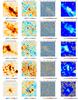 |
Fig. 24 We show the 4° × 4° regions centred around the sources listed in Table 3 in LIL and NILC y and Type 1 and Type 2 CO maps from 2015 release (Planck Collaboration XIII 2014). |
The important difference in our algorithm when compared to Aghanim et al. (2015) is that we also try to identify candidates which may be genuine clusters but with significant CO contamination so that the estimate of the y-distortion signal may not be accurate. The QN of Aghanim et al. (2015) quantifies the average contamination from all sources including dust and CIB while we focus on just one contaminant, the CO emission. Since we specifically concentrate on the CO emission foreground, our classification can be explicitly tested by using the ground based radio telescopes to look for the CO emission lines with high spectral resolution. Of course neither of the algorithms are expected to be perfect and our method is therefore complimentary to that of Aghanim et al. (2015). To summarize, out of a total of 130 clusters with S/N> 6 that we identify with annotation “MOC”, 57 are also classified by Planck Collaboration XXVII (2016) as “Bad” with QN< 0.4. While out of 72 clusters at S/N> 6 identified by Planck Collaboration XXVII (2016) as “Bad” with QN< 0.4, we identify 57 as “MOC” and 7 as “pMOC” and 3 as “IND” and 4 as “pCLG”.
The above discussion suggests an alternative path to validating and improving the reliability of the Planck cluster catalogue. This would involve using radio telescopes to measure and subtract the CO emission in the direction of cluster candidates identified by us in the Planck catalogue as MOC or pMOC. Once an accurate CO emission has been subtracted from HFI frequency maps at these locations, they can be combined to make a y map that is free of CO contamination thus confirming or denying the presence of a cluster at that location and also giving a more reliable measurement of the y-distortion amplitude. Finally we should note that our analysis suggests that the recent stacking studies of y-distortion at positions of galaxies Greco et al. (2015), Ruan et al. (2015) may also have contamination from the CO emission.
6. Conclusions
We have used a parameter fitting algorithm together with model selection to separate the y-type distortion component from the blackbody CMB and the foregrounds components in the Planck data. Using the same approach we also create a CO emission map and use a second level of model selection to identify and distinguish between y-type distortion and CO emission, assuming that in any pixel one component dominates over the other. We validate our algorithms on the real sky using known extragalactic sources of CO emission and clusters of galaxies. The result of our analysis is a minimal CO mask, which we make publicly available. We recommend this mask as the minimal mask when studying y-type distortions in Planck data. Our mask in particular includes regions of significant CO emission which might be missed by masks based solely on highest frequency HFI channels even when the masks are quite aggressive since non-negligible CO emission is coming from the molecular clouds and clumps where the dust emission is relatively weak. In addition to the y-maps free of CO contamination, our algorithm also produces CO-maps free of y-contamination and it complements the standard Dame et al. map Dame et al. (2001) by pointing out regions of high CO emission on the sky at high galactic latitudes not covered by the Dame et al map.
We revisit the Planck catalogue and find evidence of significant contamination from the CO emission, particularly in the unconfirmed candidates. Our simple approach complements the method employed by the Planck collaboration which is based on Aghanim et al. (2015). We suggest a new way of validating the Planck detected clusters by using radio telescopes to look for CO emission in the sources we have identified as molecular clouds. These observations can then be used to subtract the CO emission from Planck maps if non-zero emission is detected and get a clean y-distortion signal if there is indeed a cluster in that direction. Alternatively if no CO emission is detected then it would give confidence that the cluster is a real candidate and the usual follow-up studies can be pursued. We should clarify our identification of a source as a “MOC” just means that it is a potential target for radio observations from ground where such observation might improve the estimate and accuracy of the y-distortion signal. In particular it does not necessarily mean that there is no cluster present in that direction. A large observation program involving more than 100 scientists and targeting CO emission from molecular clouds identified in the Planck data will be underway shortly6 (Wang, priv. comm.). We have added annotations to the Planck cluster catalogue and make our annotated catalogue also publicly available7.
All masks used in this section are publicly available at http://theory.tifr.res.in/~khatri/szresults/
ESO public survey Programme ID: 196.C-0999, PI: Ke Wang, Title: Probing the Early Stages of Star Formation: Unravelling the Structure of Planck Cold Clumps Distributed Throughout the Sky, http://www.eso.org/sci/activities/call_for_public_surveys.html.
Acknowledgments
This paper used observations obtained with Planck (http://www.esa.int/Planck), an ESA science mission with instruments and contributions directly funded by ESA Member States, NASA, and Canada. I acknowledge use of the HEALPix software Górski et al. (2005) (http://healpix.sourceforge.net) and FFP6 simulations generated using the Planck sky model Delabrouille et al. (2013)http://wiki.cosmos.esa.int/planckpla/index.php/Simulation_data. This research has made use of “Aladin sky atlas” developed at CDS, Strasbourg Observatory, France Bonnarel et al. (2000). I also acknowledge useful discussions with Eugene Churazov on component separation methods. I thank Rashid Sunyaev for many useful suggestions and comments on the manuscript.
References
- Aghanim, N., Hurier, G., Diego, J.-M., et al. 2015, A&A, 580, A138 [NASA ADS] [CrossRef] [EDP Sciences] [Google Scholar]
- Akaike, H. 1974, IEEE Transactions on Automatic Control, 19, 716 [Google Scholar]
- Bonnarel, F., Fernique, P., Bienaymé, O., et al. 2000, A&AS, 143, 33 [NASA ADS] [CrossRef] [EDP Sciences] [Google Scholar]
- Challinor, A., & Chon, G. 2005, MNRAS, 360, 509 [NASA ADS] [CrossRef] [Google Scholar]
- Chon, G., Challinor, A., Prunet, S., Hivon, E., & Szapudi, I. 2004, MNRAS, 350, 914 [NASA ADS] [CrossRef] [Google Scholar]
- Dame, T. M., Hartmann, D., & Thaddeus, P. 2001, ApJ, 547, 792 [NASA ADS] [CrossRef] [Google Scholar]
- Delabrouille, J., Cardoso, J.-F., Le Jeune, M., et al. 2009, A&A, 493, 835 [NASA ADS] [CrossRef] [EDP Sciences] [Google Scholar]
- Delabrouille, J., Betoule, M., Melin, J.-B., et al. 2013, A&A, 553, A96 [NASA ADS] [CrossRef] [EDP Sciences] [Google Scholar]
- Dickey, J. M., & Lockman, F. J. 1990, ARA&A, 28, 215 [NASA ADS] [CrossRef] [MathSciNet] [Google Scholar]
- Efstathiou, G. 2004, MNRAS, 349, 603 [NASA ADS] [CrossRef] [Google Scholar]
- Eriksen, H. K., Jewell, J. B., Dickinson, C., et al. 2008, ApJ, 676, 10 [NASA ADS] [CrossRef] [Google Scholar]
- Finkbeiner, D. P., Davis, M., & Schlegel, D. J. 1999, ApJ, 524, 867 [NASA ADS] [CrossRef] [Google Scholar]
- Gold, B., Odegard, N., Weiland, J. L., et al. 2011, ApJS, 192, 15 [Google Scholar]
- Górski, K. M., Hivon, E., Banday, A. J., et al. 2005, ApJ, 622, 759 [NASA ADS] [CrossRef] [Google Scholar]
- Greco, J. P., Hill, J. C., Spergel, D. N., & Battaglia, N. 2015, ApJ, 808, 151 [NASA ADS] [CrossRef] [Google Scholar]
- Hannan, E. J., & Quinn, B. G. 1979, J. Roy. Statist. Soc. B, 41, 190 [Google Scholar]
- Hartmann, D., & Burton, W. B. 1997, Atlas of Galactic Neutral Hydrogen (Cambridge: Cambridge University Press) [Google Scholar]
- Hartmann, D., Kalberla, P. M. W., Burton, W. B., & Mebold, U. 1996, A&AS, 119, 115 [NASA ADS] [CrossRef] [EDP Sciences] [Google Scholar]
- Hartmann, D., Magnani, L., & Thaddeus, P. 1998, ApJ, 492, 205 [NASA ADS] [CrossRef] [Google Scholar]
- Hill, J. C., & Spergel, D. N. 2014, JCAP, 2, 30 [Google Scholar]
- Hivon, E., Górski, K. M., Netterfield, C. B., et al. 2002, ApJ, 567, 2 [NASA ADS] [CrossRef] [Google Scholar]
- Hurier, G., Macías-Pérez, J. F., & Hildebrandt, S. 2013, A&A, 558, A118 [NASA ADS] [CrossRef] [EDP Sciences] [Google Scholar]
- Hurier, G., Douspis, M., Aghanim, N., et al. 2015, A&A, 576, A90 [NASA ADS] [CrossRef] [EDP Sciences] [Google Scholar]
- Khatri, R. 2015, MNRAS, 451, 3321 [NASA ADS] [CrossRef] [Google Scholar]
- Khatri, R., & Sunyaev, R. 2015, JCAP, 8, 013 [NASA ADS] [CrossRef] [Google Scholar]
- Magnani, L., Blitz, L., & Mundy, L. 1985, ApJ, 295, 402 [NASA ADS] [CrossRef] [Google Scholar]
- Magnani, L., Hartmann, D., Holcomb, S. L., Smith, L. E., & Thaddeus, P. 2000, ApJ, 535, 167 [NASA ADS] [CrossRef] [Google Scholar]
- Mizuno, N., Rubio, M., Mizuno, A., et al. 2001, PASJ, 53, L45 [NASA ADS] [Google Scholar]
- Nieten, C., Neininger, N., Guélin, M., et al. 2006, A&A, 453, 459 [NASA ADS] [CrossRef] [EDP Sciences] [Google Scholar]
- Perrott, Y. C., Olamaie, M., Rumsey, C., et al. 2015, A&A, 580, A95 [NASA ADS] [CrossRef] [EDP Sciences] [Google Scholar]
- Piffaretti, R., Arnaud, M., Pratt, G. W., Pointecouteau, E., & Melin, J.-B. 2011, A&A, 534, A109 [NASA ADS] [CrossRef] [EDP Sciences] [Google Scholar]
- Planck Collaboration I. 2011, A&A, 536, A1 [NASA ADS] [CrossRef] [EDP Sciences] [Google Scholar]
- Planck Collaboration IX. 2014, A&A, 571, A9 [NASA ADS] [CrossRef] [EDP Sciences] [Google Scholar]
- Planck Collaboration XI. 2014, A&A, 571, A11 [NASA ADS] [CrossRef] [EDP Sciences] [Google Scholar]
- Planck Collaboration XII. 2014, A&A, 571, A12 [NASA ADS] [CrossRef] [EDP Sciences] [Google Scholar]
- Planck Collaboration XIII. 2014, A&A, 571, A13 [NASA ADS] [CrossRef] [EDP Sciences] [Google Scholar]
- Planck Collaboration XX. 2014, A&A, 571, A20 [NASA ADS] [CrossRef] [EDP Sciences] [Google Scholar]
- Planck Collaboration XXI. 2014, A&A, 571, A21 [NASA ADS] [CrossRef] [EDP Sciences] [Google Scholar]
- Planck Collaboration XXIX. 2014, A&A, 571, A29 [NASA ADS] [CrossRef] [EDP Sciences] [Google Scholar]
- Planck Collaboration XXIX. 2016, A&A, 582, A29 [Google Scholar]
- Planck Collaboration IV. 2016, A&A, in press, DOI: 10.1051/0004-6361/201525809 [Google Scholar]
- Planck Collaboration VII. 2016, A&A, in press, DOI: 10.1051/0004-6361/201525844 [Google Scholar]
- Planck Collaboration XXII. 2016, A&A, in press, DOI: 10.1051/0004-6361/201525826 [Google Scholar]
- Planck Collaboration XXIV. 2016, A&A, in press, DOI: 10.1051/0004-6361/201525833 [Google Scholar]
- Planck Collaboration XXVII. 2016, A&A, in press, DOI: 10.1051/0004-6361/201525823 [Google Scholar]
- Planck Collaboration Int. IV. 2013, A&A, 550, A130 [NASA ADS] [CrossRef] [EDP Sciences] [Google Scholar]
- Planck Collaboration Int. V. 2013, A&A, 550, A131 [NASA ADS] [CrossRef] [EDP Sciences] [Google Scholar]
- Planck Collaboration Int. VIII. 2013, A&A, 550, A134 [NASA ADS] [CrossRef] [EDP Sciences] [Google Scholar]
- Planck Collaboration Int. X. 2013, A&A, 554, A140 [NASA ADS] [CrossRef] [EDP Sciences] [Google Scholar]
- Planck Collaboration Int. XI. 2013, A&A, 557, A52 [NASA ADS] [CrossRef] [EDP Sciences] [Google Scholar]
- Planck Collaboration Int. XXXVI 2016, A&A, 586, A139 [NASA ADS] [CrossRef] [EDP Sciences] [Google Scholar]
- Remazeilles, M., Delabrouille, J., & Cardoso, J.-F. 2011, MNRAS, 410, 2481 [NASA ADS] [CrossRef] [Google Scholar]
- Ruan, J. J., McQuinn, M., & Anderson, S. F. 2015, ApJ, 802, 135 [NASA ADS] [CrossRef] [Google Scholar]
- Rubiño-Martín, J. A., & Sunyaev, R. A. 2003, MNRAS, 344, 1155 [NASA ADS] [CrossRef] [Google Scholar]
- Schwarz, G. 1978, Ann. Math. Statist., 6, 461 [Google Scholar]
- Stuart, A., Ord, J. K., & Arnold, S. 2004, Kendall’s Advanced Theory of Statistics, vol 2A (Sussex: John Wiley & Sons Ltd) [Google Scholar]
- Szapudi, I., Prunet, S., & Colombi, S. 2001, ApJ, 561, L11 [NASA ADS] [CrossRef] [Google Scholar]
- Tristram, M., Macías-Pérez, J. F., Renault, C., & Santos, D. 2005, MNRAS, 358, 833 [NASA ADS] [CrossRef] [Google Scholar]
- Wilson, B. A., Dame, T. M., Masheder, M. R. W., & Thaddeus, P. 2005, A&A, 430, 523 [NASA ADS] [CrossRef] [EDP Sciences] [Google Scholar]
- Wong, T., Hughes, A., Ott, J., et al. 2011, ApJS, 197, 16 [NASA ADS] [CrossRef] [Google Scholar]
- Zeldovich, Y. B., & Sunyaev, R. A. 1969, ApSS, 4, 301 [Google Scholar]
All Tables
Comparison of some clusters where our results differ from that of Aghanim et al. (2015).
All Figures
|
Fig. 1 Coma and Bullet clusters and SMC in Planck released CO Type 2 maps. Clusters show up as fake molecular clouds in J = 2− → 1 maps while strong clusters show up as negative sources in J = 1− → 0 maps. A 5 deg by 5 deg region around each source is shown. |
| In the text | |
|
Fig. 2 CO and y spectrum as seen by different Planck channels after integrating over the detector response and conversion to thermodynamic CMB temperature units. |
| In the text | |
|
Fig. 3 Map of y-type distortion at 10′ resolution constructed from the lowest four Planck HFI channels. Approximately 14.2% of the area is masked. The prominent clusters can clearly be identified. Typical contamination from the foregrounds and noise is of order ~10-6. The ring like systematic features come from the Planck scanning strategy. |
| In the text | |
|
Fig. 4 Map of CO emission at 10′ resolution constructed from the lowest four Planck HFI channels. Approximately 10.2% of the area with extremely high dust emission and clusters are masked. |
| In the text | |
|
Fig. 5 Some external galaxies with different strengths and morphology in CO emission in our y-distortion and CO maps and difference in χ2 between the two model fits. A negative value implies that CO model is favored over the y-distortion. A negative y-distortion source near M51 is a radio point source. Galactic coordinates are shown. |
| In the text | |
|
Fig. 6 Same as Fig. 5 but for the well known galaxy clusters. The |
| In the text | |
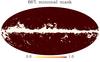 |
Fig. 7 Minimal mask covering 14.16% of the sky and used for Fig. 3. |
| In the text | |
|
Fig. 8 χ2 distribution for the parameter fits by LIL for the y-distortion model and CO model compared with the χ2 distribution for one degree of freedom. |
| In the text | |
|
Fig. 9 Some external galaxies with different strengths and morphology in CO and dust emission are compared for different component separation methods. From top to bottom the galaxies shown are M31, M33, and M82. The last row shows the Coma cluster. |
| In the text | |
|
Fig. 10 1d PDF for NILC, MILCA, and LIL y-maps for the same mask with 51% sky. |
| In the text | |
|
Fig. 11 1d PDF for NILC, MILCA, and LIL y-maps for the same mask with 51% sky and in addition with all the clusters from the second Planck cluster catalogue masked. |
| In the text | |
|
Fig. 12 Our mask with 61% sky fraction calculated using the model selection based approach described in the previous section. |
| In the text | |
|
Fig. 13 Galactic mask released by the Planck collaboration with the y-distortion maps with 58% unmasked fraction. |
| In the text | |
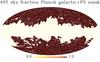 |
Fig. 14 Planck collaboration point source mask added to the galactic mask of Fig. 13. |
| In the text | |
|
Fig. 15 Comparison of different masks for the LIL y-map. |
| In the text | |
|
Fig. 16 Comparison of different masks for the NILC y-map. |
| In the text | |
|
Fig. 17 Comparison of angular power spectra of LIL, MILCA, and NILC y-maps for 60% sky fraction mask. |
| In the text | |
|
Fig. 18 Some of the candidates from Table 2 identified by our algorithm as molecular clouds or having significant contamination from the molecular clouds. |
| In the text | |
|
Fig. 19 Original Planck full channel maps smoothed to 10′ resolution at the location of the second source in Fig. 18 confirm the presence of molecular clouds in the foreground. Note that the scales in the last two maps are strictly positive. |
| In the text | |
|
Fig. 20 HI column density and Planck 857 GHz emission for the sources shown in Fig. 18. The scale of all figures is same as the respective figures in Fig. 18 with the cluster candidates from the Planck catalogue at the centre of the frame. |
| In the text | |
|
Fig. 21 One low S/N case where our test becomes unreliable visually however this preference towards it being a cluster can be inferred. |
| In the text | |
|
Fig. 22 Position on the sky in galactic coordinates of 528 sources from the Planck catalogue identified by us as likely to be clusters or indeterminable (orange circles) and 130 sources strongly likely to be molecular clouds (white triangles). |
| In the text | |
|
Fig. 23 Comparison of the two quality measures: our model selection based Δ( ∑ χ2)CO−y and QN from Planck Collaboration XXVII (2016) based on neural network based approach. |
| In the text | |
|
Fig. 24 We show the 4° × 4° regions centred around the sources listed in Table 3 in LIL and NILC y and Type 1 and Type 2 CO maps from 2015 release (Planck Collaboration XIII 2014). |
| In the text | |
Current usage metrics show cumulative count of Article Views (full-text article views including HTML views, PDF and ePub downloads, according to the available data) and Abstracts Views on Vision4Press platform.
Data correspond to usage on the plateform after 2015. The current usage metrics is available 48-96 hours after online publication and is updated daily on week days.
Initial download of the metrics may take a while.