| Issue |
A&A
Volume 591, July 2016
|
|
|---|---|---|
| Article Number | A130 | |
| Number of page(s) | 26 | |
| Section | Extragalactic astronomy | |
| DOI | https://doi.org/10.1051/0004-6361/201628595 | |
| Published online | 28 June 2016 | |
The TANAMI Multiwavelength Program: Dynamic spectral energy distributions of southern blazars⋆
1 Dr. Remeis Sternwarte & ECAP, Universität Erlangen-Nürnberg, Sternwartstrasse 7, 96049 Bamberg, Germany
e-mail: Felicia.Krauss@fau.de
2 Institut für Theoretische Physik und Astrophysik, Universität Würzburg, Emil-Fischer-Str. 31, 97074 Würzburg, Germany
3 NASA, Goddard Space Flight Center, Greenbelt, MD 20771, USA
4 University of Maryland, Baltimore County, Baltimore, MD 21250, USA
5 Catholic University of America, Washington, DC 20064, USA
6 ASTRON, the Netherlands Institute for Radio Astronomy, PO Box 2, 7990 AA Dwingeloo, The Netherlands
7 CSIRO Astronomy and Space Science, ATNF, PO Box 76, Epping, NSW 1710, Australia
8 Max-Planck-Institut für Radioastronomie, Auf dem Hügel 69, 53121 Bonn, Germany
9 Departament d’Astronomia i Astrofísica, Universitat de València, C/ Dr. Moliner 50, 46100 Burjassot, València, Spain
10 Observatori Astronòmic, Universitat de València, C/ Catedrático José Beltrán no. 2, 46980 Paterna, València, Spain
11 Departamento de Astronomía, Universidad de Concepción, Casilla 160, Chile
12 Institute for Radio Astronomy and Space Research, Auckland University of Technology, Auckland 1010, New Zealand
13 Bundesamt für Kartographie und Geodäsie, 93444 Bad Kötzting, Germany
14 CSIRO Astronomy and Space Science, Canberra Deep Space Communications Complex, PO Box 1035, Tuggeranong, ACT 2901, Australia
15 School of Mathematics & Physics, University of Tasmania, Private Bag 37, Hobart, 7001 Tasmania , Australia
16 Department ofAstrophysics/IMAPP, Radboud University Nijmegen, Heyendaalseweg 135, 6525 AJ Nijmegen, The Netherlands
17 INAF–IAPS, via Fosso del Cavaliere 100, 00033 Rome, Italy
18 Nordic Optical Telescope, Apartado 474, 38700 Santa Cruz de La Palma, Spain
19 Hartebeesthoek Radio Astronomy Observatory, Krugersdorp, South Africa
Received: 25 March 2016
Accepted: 3 May 2016
Context. Simultaneous broadband spectral and temporal studies of blazars are an important tool for investigating active galactic nuclei (AGN) jet physics.
Aims. We study the spectral evolution between quiescent and flaring periods of 22 radio-loud AGN through multiepoch, quasi-simultaneous broadband spectra. For many of these sources these are the first broadband studies.
Methods. We use a Bayesian block analysis of Fermi/LAT light curves to determine time ranges of constant flux for constructing quasi-simultaneous spectral energy distributions (SEDs). The shapes of the resulting 81 SEDs are described by two logarithmic parabolas and a blackbody spectrum where needed.
Results. The peak frequencies and luminosities agree well with the blazar sequence for low states with higher luminosity implying lower peak frequencies. This is not true for sources in high states. The γ-ray photon index in Fermi/LAT correlates with the synchrotron peak frequency in low and intermediate states. No correlation is present in high states. The black hole mass cannot be determined from the SEDs. Surprisingly, the thermal excess often found in FSRQs at optical/UV wavelengths can be described by blackbody emission and not an accretion disk spectrum.
Conclusions. The so-called harder-when-brighter trend, typically seen in X-ray spectra of flaring blazars, is visible in the blazar sequence. Our results for low and intermediate states, as well as the Compton dominance, are in agreement with previous results. Black hole mass estimates using recently published parameters are in agreement with some of the more direct measurements. For two sources, estimates disagree by more than four orders of magnitude, possibly owing to boosting effects. The shapes of the thermal excess seen predominantly in flat spectrum radio quasars are inconsistent with a direct accretion disk origin.
Key words: galaxies: active / BL Lacertae objects: general / quasars: general / relativistic processes
Tables of the fluxes are only available at the CDS via anonymous ftp to cdsarc.u-strasbg.fr (130.79.128.5) or via http://cdsarc.u-strasbg.fr/viz-bin/qcat?J/A+A/591/A130
© ESO, 2016
1. Introduction
Active galactic nuclei (AGN) are supermassive black holes at the center of galaxies that are thought to be powered by accretion (e.g., Antonucci 1993; Urry & Padovani 1995; Abdo et al. 2010a). Radio-loud AGN typically exhibit relativistic outflows of matter, called jets. Blazars constitute an ideal target for multiwavelength studies in order to understand their acceleration mechanisms and their role as potential cosmic-ray emitters. Blazars are a subclass of radio-loud AGN, with their jets oriented at a small angle to the line of sight (Blandford & Rees 1978). They emit nonthermal radiation across the whole electromagnetic spectrum (Urry & Padovani 1995) and show strong variability. Since the possible relationships between their variability in different bands is unclear, quasi-simultaneous observations are required for such studies. The radio to γ-ray spectral energy distributions (SEDs) of these sources generally show two peaks in a log ν−log νFν representation. The lower energy peak is generally attributed to synchrotron radiation from relativistic electrons in the magnetic field of the jet (see Ghisellini 2013, for a review). While both leptonic and hadronic processes likely contribute to the high-energy peak, their relative contributions remain a deeply interesting open question (Abdo et al. 2011b; Böttcher et al. 2013; Mannheim & Biermann 1992; Finke et al. 2008; Sikora et al. 2009; Baloković et al. 2016; Weidinger & Spanier 2015). In the leptonic scenario, the relativistic electrons that produce the synchrotron emission are assumed to upscatter the photons to high energies. This process is called synchrotron self-Compton (SSC). Seed photons from the ambient medium can also contribute by being upscattered to γ-ray energies (Sikora et al. 1994); this consitutes the external Compton (EC) contribution. In the hadronic scenario (e.g., Mannheim 1993), protons and electrons are assumed to be accelerated in the jet. Protons interacting with a UV seed photon field (e.g., thermal emission from the accretion disk) produce pions. Neutral pions decay into high-energy γ-rays, explaining the high-energy emission.
Based on their optical emission lines, blazars can be subdivided into flat-spectrum radio quasars (FSRQs) and BL Lacertae (BL Lac) objects. While FSRQs show broad emission lines (rest-frame equivalent width > 5 Å), BL Lacs typically show none. A few well-known exceptions include OJ 287 (Sitko & Junkkarinen 1985) and BL Lac (Vermeulen et al. 1995). Blazars can also be categorized by their synchrotron peak frequency into low, intermediate and high synchrotron peaked blazars (LSP, ISP, HSP; Padovani & Giommi 1995; Abdo et al. 2010a) with the ISP blazar peak located between 1014 Hz and 1015 Hz. Often, FSRQs exhibit a thermal excess in the optical-UV range with a temperature of ~30 000 K (Sanders et al. 1989; Elvis et al. 1994). This peak, called the “big blue bump” (BBB), is described as a broad peak, as expected from an accretion disk with a wide range of temperatures (Shields 1978; Malkan & Sargent 1982). The origin of the BBB is disputed (Antonucci 2002). Some authors argue for it to stem from the accretion disk (Shields 1978; Malkan & Sargent 1982), alternatively, free-free emission has been proposed (Barvainis 1993). The observed temperature of the feature, however, is lower than what is expected from an accretion disk (Zheng et al. 1997; Telfer et al. 2002; Binette et al. 2005). The origin of the BBB could be reprocessed accretion disk emission from clouds near the broad line region (BLR; Lawrence 2012).
While it is generally recognized that the best way to study blazars is from (near-)simultaneous broadband data (Giommi et al. 1995, 2002, 2012b; von Montigny et al. 1995; Sambruna et al. 1996; Fossati et al. 1998; Nieppola et al. 2006; Padovani et al. 2006), the lack of available simultaneous data often dictates the use of time-averaged data. In non-simultaneous SEDs, physical models can only be poorly constrained.
In addition, elevated levels of flux in the optical/UV, Fermi/LAT, or very high-energy (VHE) instruments, called “flares” or “high states”, often trigger follow-up multiwavelength observations, which lead to the availability of large amounts of quasi-simultaneous data with a paucity of comparable data in a quiescent state. Instruments observing at VHE generally have trouble detecting fainter sources (particularly FSRQs) in quiescent states. An exception is the large campaign on the low state of 1ES 2344+514 (Aleksić et al. 2013). Other campaigns involving a large number of instruments are only available for few bright sources, such as 3C 454.3 (Giommi et al. 2006; Abdo et al. 2009; Vercellone et al. 2009; Pacciani et al. 2010), Mrk 421 (Błażejowski et al. 2005; Donnarumma et al. 2009; Abdo et al. 2011b; Bartoli et al. 2016; Baloković et al. 2016), Mrk 501 (Bartoli et al. 2012; Aleksić et al. 2015; Furniss et al. 2015), 3C 279 (Grandi et al. 1996; Wehrle et al. 1998; Hayashida et al. 2015; Paliya et al. 2015), BL Lac (Abdo et al. 2011a; Wehrle et al. 2016), S5 0716+714 (Rani et al. 2013; Liao et al. 2014; Chandra et al. 2015), and PKS 2155−304 (Aharonian et al. 2009; Abdo et al. 2010a).
In this study we used data from the TANAMI multiwavelength project (Kadler et al. 2015) to construct quasi-simultaneous broadband SEDs for high-energy (HE) γ-ray bright southern blazars. These SEDs include several epochs at different flux levels and have good spectral coverage. We selected the 22 TANAMI blazars that were brightest in the Fermi/LAT band and constructed a total of 81 SEDs with good coverage across the entire spectrum. We obtained SEDs in low, intermediate, and high states for several sources. We used this large sample of SEDs to study the spectral evolution over time, the blazar sequence, Compton dominance, fundamental plane of black holes, and the big blue bump.
The paper is structured as follows. In Sect. 2 we introduce the sample used and its limitations and describe the multiwavelength data and their extraction and analysis. We also include the method of constructing the broadband SEDs, how systematic uncertainties are treated, and caveats of our method. In Sect. 3 we present the results from the broadband fits including results pertaining to the blazar sequence, Compton dominance, thermal excess, and fundamental plane of black holes. We summarize and discuss the results in Sect. 4.
Throughout the paper we use the standard cosmological model with Ωm = 0.3, Λ = 0.7, H0 = 70 km s-1 Mpc-1 (Beringer et al. 2012).
Sources used in the SED catalog.
2. Generation of contemporaneous broadband spectral energy distributions
2.1. Sample selection
The Tracking Active Galactic Nuclei with Austral Milliarcsecond Interferometry (TANAMI1; Ojha et al. 2010 sample includes ~100 AGN in the southern sky at declinations below −30°. It is a flux-limited sample, covering southern flat spectrum sources with catalogued flux densities above 1 Jy at 5 GHz, as well as Fermi detected γ-ray loud blazars in the region of interest. These sources are monitored by TANAMI with Very Long Baseline Interferometry (VLBI) at 8.4 GHz and 22 GHz (X-band and K-band, respectively). In addition to the VLBI monitoring, single dish observations are performed at several additional radio frequencies with the ATCA and Ceduna. These radio observations are complemented with multiwavelength observations, primarily with Swift and XMM-Newton in the X-rays, and the Rapid Eye Mount (REM) telescope at La Silla in the optical. The TANAMI sample is regularly extended by adding bright sources newly detected by Fermi/LAT (Böck et al. 2016).
As a result of the good coverage in wavelength and time, the TANAMI sample is ideal for a study of the behavior of blazar SEDs. Previous studies include detailed studies of the blazars 2142−758 (Dutka et al. 2013), 0208−512 (Blanchard 2013), and PKS 2326-502 (Dutka, submitted).
In this paper we study the multiwavelength evolution of the 22 γ-ray brightest TANAMI sources according to the 3FGL catalog (Acero et al. 2015). Our results are therefore representative of a γ-ray flux-limited sample. The 22 sources are listed in Table 1. We include the IAU B1950 name, 3FGL association, 3FGL catalog name, source classification that we used, the redshift, right ascension and declination, the Galactic absorbing column in the direction of the source and, finally, the number of SEDs that we were able to construct for each of the sources. Our sample includes nine BL Lac type objects, 11 FSRQs, and two blazars of unknown type. The brightness of these sources enabled us to extract Fermi/LAT light curves with 14-day binning. For some of these sources, these are their first broadband SEDs in the literature. While an optical classification of most sources is relatively easy, some sources have contradictory classifications in different AGN catalogs. These are labeled as blazar candidates of unknown type (BCU). One example is 0208−512. In the CGRaBS survey of bright blazars (Healey et al. 2008), this source was listed as a BL Lac type object in agreement with the optical classification from the 12th catalog of quasars and active nuclei (Véron-Cetty & Véron 2006). It was classified as a FSRQ, however, based on optical emisison lines by Impey & Tapia (1988). The 5th Roma BZCAT lists the source as a BZU (blazar of uncertain or transitional type) and describes it as a transition object, but lists it as an FSRQ (Massaro et al. 2009). Possible misclassifications did not change any of our results, as we generally did not treat the two populations differently and find many of the results are not dependent on the source classification. A redshift of 1.45 is often used for 0332−403 (Hewitt & Burbidge 1987), but Shen et al. (1998) point out that the origin of this value is unknown. It is further worth noting that 0521−365 is often not considered a blazar, but regarded as a transitional object between a broad line radio galaxy and a steep spectrum radio quasar with a VLBI morphology similar to a misaligned blazar (D’Ammando et al. 2015).
Having selected the sources, we generated contemporaneous broadband SEDs for observational periods where our sources were determined to be at a relatively constant level of γ-ray activity. These periods are determined using a Bayesian blocks analysis of Fermi/LAT light curves (Sect. 2.2), for which we then searched for contemporaneous observations in other energy bands (Sect. 2.3).
2.2. Fermi/LAT light curve analysis
The lack of simultaneous observation campaigns on most sources means that we often have to rely on quasi-simultaneous data when assembling the SED for an AGN. These SEDs are only representative of the true SED if the data included are from times when the source emission did not change appreciably. With the launch of Fermi in 2008, we have access to continuous γ-ray light curves of blazars, which are ideal for identifying flux states and applying a criterion to separate the data into time ranges of similar flux.
We calculated Fermi/LAT (Atwood et al. 2009) light curves for the time period August 4, 2008 through January 1, 2015 using the reprocessed Pass 7 data (v9r32p5) and the P7REP_SOURCE_V15 instrumental response functions (IRF; Ackermann et al. 2012) and a region of interest (ROI) of 10°. The data were separated into time bins of 14 d, on which we perform a likelihood analysis. The input model is based on point sources from the 3FGL catalog (Acero et al. 2015) and further includes spatial and spectral templates for the Galactic (gll_iem_v05_rev1) and isotropic (iso_source_v05) diffuse emission. The first step was to define a criterion for the time ranges. A wide variety of methods are used for defining quasi-simultaneity in multiwavelength studies. Some studies utilize a flux or count rate threshold (Błażejowski et al. 2005), and other methods include fixed time bins (Giommi et al. 2012b; Carnerero et al. 2015; Tagliaferri et al. 2015), double exponential forms that are fit to the light curve (Valtaoja et al. 1999; Abdo et al. 2010b; Hayashida et al. 2015), and “by eye” definitions (Tanaka et al. 2011; D’Ammando et al. 2013). These methods are either model dependent or do not take the amount of variation into account. A source might show strong, nondiscrete variations during a flare, which are not separated. These variations are not useful for studying quiescent SEDs either.
We decided to choose time ranges based on a statistical tool known as the Bayesian blocks algorithm. The Bayesian block method is nonparametric, i.e., the data are not described by a model and evaluated. Local (nonperiodic) variability in the light curve is found with a maximum likelihood approach by determining change points where the flux is inconsistent with being at a constant level (Scargle 1998; Scargle et al. 2013). Using an Interactive Spectral Interpretation System (Houck & Denicola 2000) adaption of the code of Scargle et al. (ISIS; 2013, M. Kühnel, available online2, we found the global optimum division of the light curve into segments of constant flux. While this assumption of states of constant flux is in reality not correct, as sources rarely vary in a discontinuous way, this approach is still very powerful in identifying time ranges of source “states” where the flux is at least statistically constant. Here we adapted a significance of the change points at the 95% confidence level. Such a relatively low value was chosen as we want to keep the number of false negatives (where real changes in flux are missed) low. Introducing a low number of false positives, where constant flux is seen as a change point, however, does not harm our analysis. If a constant flux is interpreted as a change point, it segments the data more than necessary. In the worst case this could lead to two missed broadband spectra if, through the segmentation, the multiwavelength data in either time range is not sufficient for constructing a broadband SED. Based on the 95% confidence level, we estimate that out of the 81 SEDs, only ~4 are based on a false-positive detection of a change in flux. The Fermi/LAT light curves are shown in Appendix A.1. The Fermi/LAT data points are shown in black, while the segmentation by the Bayesian blocks is shown in dark gray. The average flux across the whole light curve is shown in pink. We additionally show available multiwavelength data above the light curve at the corresponding times of the observations. Blocks with a sufficient amount of multiwavelength data are indcated in color and are labeled with Greek letters.
We ensure that the flux at γ-ray energies is statistically constant, but no such criterion can be applied to other wavelengths because of a lack of good cadence observations. It is possible that variability in the X-ray, optical, or radio band is missed in Fermi/LAT and averaged over or completely absent. This effect might contribute to the problems of broadband fitting. Typically blazar monitoring has shown that often the largest and fastest relative changes in flux occur at high and very high-energy γ-rays. Variability in the radio occurs on much longer timescales, which is consistent with the outward traveling of material from the base of the jet and becoming optically thin at different locations.
2.3. Quasi-simultaneous time periods
As a result of the large uncertainty of individual flux measurements in fainter AGN, the Bayesian blocks analysis can yield segments longer than a year during which the γ-ray flux is found to be statistically constant. This behavior can hide true variations in flux. We therefore subdivided Bayesian blocks into a new size if they are longer than one year, depending on their Fermi/LAT flux in the time range. The new blocks are at least (2, 5, 10, 25, or 42) × 14 d bins in size, if the Fermi/LAT flux in the time range is greater than 1 × 10⁻⁶, 0.5 × 10⁻⁶, 1 × 10⁻⁷, or 1 × 10⁻⁸ ph s-1 cm-2, respectively. This selection of fluxes and time bins accounts for longer integration time needed for a source with low flux to obtain a Fermi/LAT spectrum of good quality, and is based on experience. For a time bin of 370 d duration with a flux of 2 × 10⁻⁷ ph s-1 cm-2, for example, the new time range would be 10 × 14 d = 140 d. We obtained 370 d/140 d = 2.64 new bins for this new block size, which means that we subdivided the original interval into ⌊ 2.64 ⌋ = 2 bins with a length of 185 days each.
Time periods that include γ-ray, X-ray, optical, and VLBI observations are then used for quasi-simultaneous SEDs. Earlier works have shown that the radio flux varies on longer timescales than the γ-rays (Soldi et al. 2008). We therefore also included time periods that have γ-ray, X-ray, and optical data in the same block, as well as VLBI observations inside the block, or close to the block start or end. Close to the block is defined as within a time range 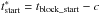 and
and 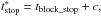 where c = max { 0.6Δt,50 d } and where Δt is the length of the block. The smaller value, 50 d, was chosen because the radio emission varies on much longer timescales. Therefore, even for a very short block of 14 days, for example, it is acceptable to use radio data 50 days prior to the start of the block. For longer time periods of quiescence, it is acceptable to use VLBI data that is offset from the start or to stop of the block by 60% of the block length. The value 60% is arbitrary based on the variability timescales of the VLBI flux. In the case of the previous example, Δt = 185 d and therefore c = 111 d, such that radio data from an interval of 111 d + 185 d + 111 d = 407 d length would be considered. The considered time range was this large in only a small number of sources. In sources with large error bars, considerable time averaging had to be performed to obtain a good quality Fermi/LAT spectrum. This is why the original sample was limited to ensure that time averaging is only necessary in a few cases. Thus the time interval exceeds 365 days in 24 of the 81 SEDs.
Blocks can be divided, according to their average flux ranges, into three categories: high, intermediate, and low flux states. We compared the flux in a block with the average flux across the whole light curve to determine its “state”. Blocks with a flux between 0.8 and 1.5 of their average flux were labeled as intermediate states. The number of SEDs with the source in the low state is relatively small. As expected, sources were found to be close to their average flux most of the time. In the high state, the large number of triggers on such flaring blazars and the higher overall source flux allow for better statistics.
2.4. Fitting strategy
Having selected the time intervals with sufficient data, we extracted broadband spectra for each interval. Broadband fitting is generally performed on energy flux spectra in the νFν-representation. This approach is very problematic, however, especially in the X-ray and γ-ray regime, as the low spectral resolution of the instruments used in these bands makes it mathematically impossible to recover the source spectral shape and flux in an unambiguous way by “unfolding” (e.g., Lampton et al. 1976; Broos et al. 2010; Getman et al. 2010). These “unfolded” flux densities are in general biased by the shape of the spectral model that was used in obtaining them (Nowak et al. 2005). For very broad energy bands and strongly energy-dependent spectra, which are present in blazar spectra, the unfolded flux densities can be in error by a factor of a few. To avoid these problems, we used ISIS (ISIS; Houck & Denicola 2000) and treat all data sets in detector space. ISIS allows us to use data with an assigned response function (e.g., Swift/XRT and Swift/UVOT data) in combination with data that are only available as flux or flux density, such as the radio data, some of the optical data sets, or Fermi/LAT data. A diagonal matrix was assigned to those without an available response function. All data modeling was performed in detector space; we use unfolded data only for display purposes. We use the model-independent approach discussed by Nowak et al. (2005) for the unfolding. As this approach is still biased by assuming a constant flux over each spectral bin, the residuals shown in our figures, which were calculated in detector space, can disagree with the photon data converted to flux values.
We further caution that the methods used to obtain the fluxes in the different energy bands are not identical. The Fermi/LAT fluxes and most of the optical data points are model dependent, while the X-ray, Swift/UVOT, and XMM-Newton/OM fluxes are model independent. These uncertainties should be covered by the added systematic uncertainties, which are described in the following.
The data reduction approach performed for the instruments entering our analysis is as follows:
-
Fermi/LAT:
We calculate Fermi/LAT spectra for the indi-vidual time periods as determined from the Fermi/LAT lightcurve. The adopted systematic uncertainty of the flux is 5%,due to approximations in the instrumental response function(IRFs) and uncertainties in the PSF shape and the effectivearea3.In addition, to show the average γ-ray flux, our SED figures also show unfolded spectra from the 3FGL, which cover the time period 2008 August to 2012 July.
-
Swift/XRT:
Swift (Gehrels et al. 2004) data are from a TANAMI fill-in program and were supplemented with archival data. The data were reduced with the most recent software package (HEASOFT 6.17)4 and calibration database. For the windowed timing/photon counting mode a systematic uncertainty of 5%/10% has been adopted following Romano et al. (2005).
-
XMM-Newton/pn and MOS:
Data from the three CCDs on XMM-Newton (Turner et al. 2001; Strüder et al. 2001) were reduced using the SAS 14.0.05. According to the official calibration documentation6, uncertainties in the absolute flux calibration are up to 5%, which we used as the systematic uncertainty for the pn detector and the MOS cameras.
-
Swift/UVOT:
The UVOT data are from the same observations as the Swift/XRT data. They were reduced with the most recent version of HEASOFT using standard methods. The systematic uncertainty for the Swift/UVOT detector is 2%. Contributions to the uncertainty include the change in filter sensitivity, i.e., the effective area. The uncertainty due to coincidence loss is less than 0.01 mag (less than 1%; Breeveld et al. 2005; Poole et al. 2008; Breeveld et al. 2010, 2011).
-
XMM-Newton/OM:
The systematic uncertainty of the XMM-Newton/OM was determined to be ~0.1 mag. This value does not include the uncertainty in the zero points. We therefore used 3% as an estimate of the combined systematics7.
- SMARTS:
SMARTS is an optical/IR blazar monitoring program using the SMARTS 1.3 m telescope, and ANDICAM at CTIO (Bonning et al. 2012). This program monitors bright southern Fermi/LAT blazars on a monthly basis. The photometric systematic uncertainty for the SMARTS program is ~0.05 mag with deviations up to 0.1 mag. We therefore used 0.07 mag for the systematic uncertainty, but it does not include the uncertainty in the zero points. Bonning et al. (2012) uses the zero points given by Persson et al. (1998) and Bessell et al. (1998) for the J filter, which gives a value of 1589 mJy. Buxton et al. (2012) use the value from Frogel et al. (1978) and Elias et al. (1982), which is given as 1670 mJy. We used the value by Elias et al. (1982).
- REM:
Based on photometry, the systematic uncertainty is 0.05 mag (R. Nesci, priv. comm.). This value does not include the uncertainty of the zero points.
TANAMI VLBI observations were performed with the Australian Long Baseline Array (LBA) in combination with telescopes in South Africa, Chile, Antarctica, and New Zealand at 8.4 GHz. Details of the correlation of the data, the subsequent calibration, imaging, and image analysis can be found in Ojha et al. (2010). We used the TANAMI core fluxes in our multiwavelength analysis, which excludes flux contributions from the extended jet in the case of noncompact sources. Contributions to the SED at X-ray and γ-ray energies is expected to originate from the inner regions, close to the base of the jet. Core radio fluxes are therefore expected to be representative of the same region as the high-energy data. The statistical errors of VLBI flux measurements are currently not well determined. We added a conservative 20% flux uncertainty that covers statistical and systematic errors. TANAMI VLBI observations are supported by flux-density measurements with the Australia Telescope Compact Array (ATCA; Stevens et al. 2012) and the Ceduna 30 m telescope (McCulloch et al. 2005).
Data from the following instruments are shown in the SED figures in Appendix A to better illustrate the average spectral shape of the sources. They were not included in the spectral fits since no time selection was possible on these data sets.
-
INTEGRAL:
Spectra for two of the 22 sources were includedfrom the HEAVENS online tool (Winkleret al. 2003; Walteret al. 2010). The data aredominated by Poisson statistics and no systematic errors had to beadded.
-
Swift/BAT:
BAT data are based on updated 104-month BAT survey maps (see Baumgartner et al. 2013, for a description of the BAT survey). No calibration uncertainty for the flux values are given for the Swift/BAT instrument. We added an uncertainty of 0.75% to the Swift/BAT data, following the uncertainty quoted by Baumgartner et al. (2013) for broadband BAT light curves.
-
Wide-Field Infrared Survey Explorer (WISE):
data from the ALLWISE catalog (Wright et al. 2010) are in the infrared waveband. Contributions to the photometric uncertainty of WISE data include source confusion (negligible outside the Galactic plane), uncertainty in zero points and in background estimation, and uncertainty of the photometric calibration (~ 7%8; Wright et al. 2010). The uncertainty of the zero points depends strongly on the filter. It lies between 4 and 20% (for W4)9. We used an average uncertainty of 14.5% and apply the correction factor appropriate for a Fν ∝ ν-1 spectrum in the conversion of magnitudes to fluxes (Wright et al. 2010).
-
2MASS:
the 2MASS point source catalog (PSC; Skrutskie et al. 2006) photometric uncertainty is hard to determine, as the data were taken over many months, with varying weather, seeing, atmospheric transparency, background, and moonlight contamination. The average uncertainty is quoted as 0.02 mag for bright sources above a Galactic latitude of 75°10. we used a systematic uncertainty of 0.05 mag to account for other latitudes. This value does not include systematic uncertainties of the zero points.
-
Planck:
we included the aperture photometry values from the Planck Catalog of Compact Sources (Planck Collaboration XXVIII 2014) for information purposes only. Above 100 GHz, sources outside the Galactic plane have a contamination from CO of up to 6%. The photometric calibration uncertainty is less than 1% below 217 GHz and less than 10% at frequencies between 217 GHz and 900 GHz (Planck Collaboration XXVIII 2014). We added an uncertainty of 10% to the Planck data to account for the CO contamination and the photometric calibration uncertainty.
2.5. Fitting the broadband spectrum
The aim of this paper is to obtain an overall understanding of the spectral behavior of our source sample and how it depends on primary source parameters. Physical models often have the problem of a large number of unknown parameters such as the black hole mass, jet properties, etc. (e.g., Böttcher et al. 2013), which lead to significant correlations between individual parameters. We describe the data with the empirical logpar model (Massaro et al. 2004), a parabola in log Fν-log ν-space. The logpar model 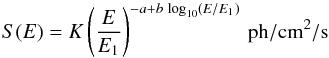 (1)is parametrized by its normalization K, the photon index a at the energy E1, and the curvature of the parabola b at energy E1.
Two parabolas were necessary to describe the low and high-energy hump. This continuum is modified by absorption and extinction (tbnew and redden, respectively) and by a blackbody component where necessary. The final model in ISIS-syntax is  (2)where Nph(E) is the photon flux. The curvature and slope of the logarithmic parabolas are strongly correlated. When deriving the peak frequency and peak flux/luminosity and their respective errors, error propagation overestimates the resulting uncertainty of these parameters. The resulting errors are often larger than the values, thus conveying no useful information, as it is very unlikely that the peak error is larger than more than two orders of magnitude. The error bars have therefore been omitted from the plots in the results section where they are not useful. We estimated the true uncertainty by shifting the peak position and comparing the χ2 values. For sources with good to average coverage, the total uncertainty is small (~half an order of magnitude). The total uncertainty is one order of magnitude for sources with missing coverage close to the peak. This is shown in the lower left corner of the corresponding figures. It is harder to determine the uncertainty for the Compton dominance, and we conservatively estimate an order of magnitude.
The blackbody(1) component in Eq. (2)describes the BBB, an excess at optical to ultraviolet wavelengths that was first seen in 3C 273 (Shields 1978). In some sources (e.g., Seyfert galaxies, and some BL Lac objects) with weak continuum emission, the emission of the host galaxy is not outshone by the nonthermal continuum emission (e.g., NGC 4051, Maitra et al. 2011). This feature is very similar in shape to the BBB, but located at lower energies, corresponding to lower temperatures of ~ 6000 K. The origin of the BBB at higher temperatures of ~ 30 000 K is still debated. In many studies of blazar SEDs, the BBB is treated as background to the nonthermal emission and is often assumed to be the accretion disk. Typically this feature is visible in FSRQs (Jolley et al. 2009, and references therein). In this work, we modeled the BBB emission with a single-temperature blackbody. In a few cases, a multi-temperature blackbody diskbb model, i.e., emission from an accretion disk with T(r) ∝ r− 3/4 (Mitsuda et al. 1984; Makishima et al. 1986) is required to describe the BBB shape. Figure 1 shows an example of the complete model.
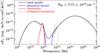 |
Fig. 1 Broadband spectral model of 0402−362 with two logarithmic parabolas including reddening and absorption (blue), a dereddened and reddened blackbody (red, red dashed), and the total unabsorbed model (black). |
Because of the very distinct features imposed by interstellar absorption in the X-ray band, in our spectral fits we first determined the hydrogen equivalent column, NH, from a power law fit to the X-ray data only. Such a simple absorbed power law fit worked well in almost all of the cases and no source with a large excess above the Galactic NH was found. In the final broadband fits, we fixed the absorbing column NH to the value determined by the best fit to the X-ray data or to the Galactic 21 cm value. The Galactic absorption was used if the best-fit χ2 was high, or the best-fit value consistent with the Galactic 21 cm value. As the extinction at infrared, optical, and UV wavelengths is due to the same material that absorbs X-rays, we modeled the optical extinction based on the NH value that is used for the X-ray data, converting it to AV from X-ray dust scattering halo measurements of Predehl & Schmitt (1995) as modified by Nowak et al. (2012) for the revised abundance of the interstellar medium. This approach worked very well, contrary to many works that require an optical extinction correction that is separate from the X-ray modeling. We speculate that this is because these investigation used the original Predehl & Schmitt (1995) formulae and therefore obsolete abundances.
We caution that a possible uncertainty exists in the fit to the X-ray data, which often have large errors (~ 50%) as a result of short exposure observations by Swift/XRT. The Galactic value from the LAB survey has an uncertainty of ~30%, due to stray radiation, unresolved structures, and the assumption of optical transparency (Kalberla et al. 2005). An additional problem is that the X-ray modeling assumes a fixed (Galactic) abundance, which might be the wrong assumption for the absorption in the host galaxy.
Occasionally, the lack of data necessitated some parameters to be fixed at a typical value in order to find a good fit, especially for high-peaked BL Lac sources, where the peak of the high-energy hump lies above Fermi energies and is not covered by our data. It was not possible in these cases to constrain the curvature of the parabola well from the data. Further, because of scarce data around the peak frequencies (typically in the sub-mm and MeV range), the exact spectral shape of the two bumps is unclear. Although the two log-parabolas work remarkably well here and an averaged spectrum of 3C 273 (Türler et al. 1999) is remarkably parabola-like in shape, some physical models predict steep bends or additional components (Mannheim 1993; Böttcher et al. 2009). In addition, in a few cases, such as 1424−418, the parabola shape did not describe the data well, especially the high-energy hump, as the X-ray spectrum is harder than what is expected from the parabola fit.
We use a χ2 approach to determine the goodness-of-fit. This method is not statistically sound, as the errors on the VLBI data are only estimated and they are likely too large. In relative terms, the (reduced) χ2 values still give a good estimate of the goodness-of-fit, but are not indicative of an absolute goodness-of-fit, i.e., in the probability of the model.
3. Results and discussion
Based on the methods outlined above, we fitted all 81 spectra with the spectral model of Eq. (2). Of the 22 sources 12 have more than two quasi-simultaneous SEDs, and ten have only two quasi-simultaneous SEDs. The fit results are listed in Table A.1. The table shows that even though the logarithmic parabolas are not a physical model, they can describe the broadband behavior very well, reaching low χ2 values. While this does not indicate the probability of the model, the relative reduced χ2 values give an estimate of the goodness-of-fit. It is surprising that they reach low values as many instruments are not flux cross-calibrated. We note that FSRQs tend to have an index that is too soft to describe the Swift/XRT and Fermi/LAT spectrum perfectly. In some sources the LAT spectrum constrains the curvature of the parabola well, for which the X-ray spectral indices are too soft (see, e.g., 1424−418). The reason for this behavior might be from a spectral break in the MeV energy range. Other possibilities include an accretion disk component in the soft X-rays or a pion decay signature at MeV energies.
We find one source, 2005−489, with a peculiar excess in the hard X-rays above 5 keV, which can be described with a thermal blackbody, but likely only due to a lack of data above 10 keV. It might be possible to explain this with a hadronic proton-synchrotron signature, but the origin is as yet unclear (see Sect. 3.5).
In the following sections we describe the behavior of individual parameters in greater detail. For some sources the redshift is unknown. While all broadband SEDs are modeled without k-corrections, the analysis, e.g., of source fluxes or peak positions often requires knowledge of the redshift. Sources without redshifts are therefore not included in the results, unless noted otherwise.
3.1. The peak positions
3.1.1. Blazar sequence
The blazar sequence posits that more luminous blazars have lower peak frequencies (Fossati et al. 1998; Ghisellini et al. 1998). While it is heavily debated (e.g., Giommi et al. 2012a,b), it is generally observed for most sources with known redshift, although sources with low luminosities at low peak frequencies have been found (Nieppola et al. 2006; Meyer et al. 2011; Giommi et al. 2012a). Sources at high luminosities and high peak frequencies are still missing, however, possibly owing to the lack of redshift information. Meyer et al. (2011) propose a modified blazar sequence, where more luminous blazars are more efficient at accretion. Sources with lower peak luminosities and higher peak frequencies than expected are interpreted as misaligned, leading to a shift in the peak.
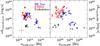 |
Fig. 2 Peak frequency (k-corrected) and peak luminosity for the synchrotron peak (left) and the high-energy peak (right). The estimated uncertainty is given in the lower left corner for sources with average coverage (orange) and for SEDs with a lack of data near the peak position (gray). |
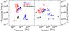 |
Fig. 3 “Inverted blazar sequence”: HE peak luminosity (left) vs. peak synchrotron frequency (k-corrected) and vice versa (right). The estimated uncertainty is given in the lower left corner for sources with average coverage (orange) and for SEDs with a lack of data near the peak position (gray). |
Figure 2 shows the k-corrected peak frequencies and peak luminosities for all 20 sources in our sample for which a redshift measurement is available. The synchrotron peak results are consistent with the blazar sequence with a gap between 1014 and 1015 Hz. This gap was also seen in 3LAC (Ackermann et al. 2015) and was named the Fermi blazars’ divide (Ghisellini et al. 2009). See Sect. 3.2 for a further discussion of this feature.
We also find one source, 0521−365, with a lower peak frequency and peak luminosity than expected from the blazar sequence. It is interesting to note, but likely a coincidence, that the peak of this source is perpendicular to the blazar sequence at the location of the gap.
While the positions of the high-energy peak seem to generally follow the blazar sequence, the spread is much wider, which is consistent with expectations from a SSC model. When “inverting” the blazar sequence by looking at the synchrotron peak frequency versus the HE peak luminosity, it still follows the blazar sequence. The opposite is not true (Fig. 3). The HE peak frequency vs. the synchrotron luminosity shows a rising and falling slope (or a V-shape flipped on the horizontal axis), which, when going back to the regular blazar sequence, might also be visible there.
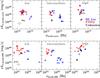 |
Fig. 4 Peak frequencies and peak luminosities, separated into low, intermediate, and high states for the synchrotron peak (top row) and high-energy peak (bottom row). While the low and intermediate states follow the blazar sequence for both peaks, the high-energy peak in both states show a peculiar, almost inverted behavior, although the number of sources (especially BL Lacertae objects) is too low for any conclusive evidence. The estimated uncertainty is given in the lower left corner of the left panels for sources with average coverage (orange) and for SEDs with a lack of data near the peak position (gray). |
Figure 4 shows the blazar sequence separated by the activity of the source at a given time. The upper panel shows the location of the synchrotron peak, and the lower panel shows the position of the high-energy peak. Both panels are separated into low, intermediate, and high states. We find that in the intermediate state (and possibly in the low state), the sources follow the blazar sequence (Fig. 2). In the high state the synchrotron peak results are inconclusive and seem to scatter. We find, as previously seen, that high-peaked BL Lac objects show a much lower occurrence of large outbursts in HE γ-rays, and our sample includes no high-peaked SED (above 1014.5 Hz) in a high state. Even when we take this lack of data into account, the blazar sequence slope of the high-energy peak in the high state is drastically different from the intermediate state, possibly showing an increase in peak frequency with peak luminosity.
To see whether this behavior is statistically significant, we also looked at individual behavior. We find that in the intermediate state the high-energy peak tends to move toward lower frequencies, while it moves toward higher frequencies in high states. This behavior is discernible for the sources 0521−365, 0537−441, and 1454−354. For 0208−512, 0332−376, 0426−380, and 0402−362 only one of the effects is visible, likely because of a lack of data (see Fig. A.2). No disagreeing trends were found for the other sources, but some SEDs lack information from all states, for example, 0402−362 only has two high state SEDs, so no information about the peak shift is available. While this behavior has not been documented for a large sample, a “harder-when-brighter” trend is often seen in the X-ray spectra of flaring blazars and other AGN consistent with a peak shift to higher frequencies (Zamorani et al. 1981; Avni & Tananbaum 1982; Pian et al. 1998; Vignali et al. 2003; Emmanoulopoulos et al. 2012). For a number of flaring Fermi/LAT sources, a hardening of the spectral index has also been observed (Abdo et al. 2010c,d), which might be useful in the future for discriminating between intermediate and flaring states, though no physical explanation is readily available.
3.1.2. Spectral index and peak position
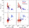 |
Fig. 5 Behavior of the synchrotron (left) and HE (right) peak frequency as a function of the photon index seen in the Fermi/LAT (top) and Swift/XRT bands (bottom). |
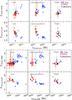 |
Fig. 6 Synchrotron (top) and HE (bottom) peak frequency vs. the photon index seen by Swift/XRT (top) and Fermi/LAT (bottom) separated by low, intermediate, and high states. |
The correlations between the spectral indices seen in Fermi/LAT and Swift/XRT and the synchrotron peak frequency, are documented well in the 3FGL catalog (Acero et al. 2015). Correlations with the high-energy peak are less studied. All spectral indices are shown in Fig. 5, and in Fig. 6 they are separated into low, intermediate, and high states. The top panel of the figure shows the synchrotron peak frequency versus the XRT and LAT indices, while the lower panel shows the high-energy peak frequency versus the XRT and LAT indices. It is interesting to note that the LAT index shows varying behavior in the bottom panel of the top plot (synchrotron peak frequency) in Fig. 6, depending on source state, but not in the bottom panel of the bottom plot (HE peak frequency). This change in the high state is consistent with a difference in synchrotron and high-energy peak behavior of the sources. In the low and intermediate states, the LAT index shows a correlation with the synchrotron peak frequency, indicative of correlated processes. The data seems more scattered for SEDs in the high state. This change is indicative of a change in the jet properties during a high state, such as an acceleration of the jet flow (Marscher et al. 2010).
3.1.3. Compton dominance and the blazar sequence
Giommi et al. (2012b) suggest that the blazar sequence is due to the selection bias of the observed samples. The sources missing in the blazar sequence are expected to peak in the optical/UV. These sources should be the brightest among the optical-selected blazars. Giommi et al. (2012b) argue that these sources are dominated by jet emission in the optical, making it nearly impossible to determine their redshift spectroscopically. The argument is therefore that these sources exist, and are known, but no luminosities are available. Therefore, Finke (2013) uses the Compton dominance, Fpeak,HE/Fpeak,sync, a redshift independent quantity to verify the existence of the blazar sequence, and also finds a lack of sources at high peak frequencies and luminosities.
While we might miss low luminosity sources in the TANAMI sample, we would expect to have found sources with high luminosities at high peak frequencies if they exist. These are expected to be bright and have hard spectral indices in Fermi/LAT. As our sample is representative of a γ-ray flux-limited sample, it is possible that we miss bright sources peaking in the optical if their Compton dominance is low, i.e., if their high-energy peak is faint, possibly even fainter than the synchrotron peak.
Consistent with earlier findings (Giommi et al. 2012b; Finke 2013), Fig. 7 shows that there is a redshift-independent correlation between the ratio of the peak fluxes and the peak frequency. The sequence can be explained physically by increasing power leading to larger external radiation fields and a larger Compton dominance. Higher Compton scattering leads to faster cooling and a lower cutoff of high-energy photons, possibly explaining the observed blazar sequence.
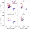 |
Fig. 7 Top left: Compton dominance for all SEDs for all sources (no k-correction). The blazars’ divide is particularly strong; only few sources are found between 1014 and 1015 Hz. Top right and bottom: same as above, but SEDs are separated into low, intermediate, and high states. The estimated uncertainty is given in the lower left corner of the top right panel in gray. |
Looking at the state separated behavior (Fig. 7, bottom and top right), while the number of SEDs in the high state is low, the behavior during high states is different from the low and intermediate states. As for the blazar sequence, the low and intermediate states are consistent with expectations from the blazar sequence and FSRQs at higher Compton dominances. In the high state, the Compton dominance shows a large scatter. We further generate the Compton dominance for the bolometric fluxes, instead of the peak flux.
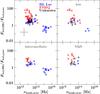 |
Fig. 8 Top left: bolometric Compton dominance for all SEDs for all sources (no k-correction). The blazars’ divide is particularly strong. Top right and bottom: same as above, but SEDs are separated into low, intermediate, and high states. The estimated uncertainty is given in the lower left corner of the top right panel in gray. |
The bolometric fluxes are calculated by integrating over each of the two best-fit parabola functions separately (Fig. 8). The patterns in Figs. 7 and 8 are very similar. While the scatter is lower when using bolometric fluxes, it shows that the peak position is a reliable tracer of the bolometric flux.
3.2. The Fermi blazars’ divide
In the blazar sequence and Compton dominance a large gap is visible, which seems to separate FSRQs and BL Lac objects between 1014 and 1015 Hz. This gap has also been seen in the 3LAC (Ackermann et al. 2015) and is now named the Fermi blazars’ divide, as first discussed by Ghisellini et al. (2009). These authors propose a physical difference in these objects with a separation of objects into low and high efficiency accretion flows. In our γ-ray flux limited sample, however, this separation is much stronger than in the 3LAC, suggesting a contribution of selection effects. These selection effects can contribute in the same way as to the blazar sequence, i.e., we would expect a lack of redshifts in objects peaking in the optical range (1014–1015 Hz), which would show a featureless spectrum due to a dominant jet component. Furthermore, the extinction in the UV and far UV, as well as the photoelectric absorption of soft X-rays in our Galaxy, hamper the detection of blazars peaking in this energy range, which are exactly those peak frequencies missing in the blazars’ divide. We expect that this can fully explain the Fermi blazars’ divide and is also consistent with observations of black hole binaries, which do not show a gap between accretion states.
Selection effects are able to explain the blazars’ divide, while the argument is less clear for the blazar sequence, which is found even in the Compton dominance, which is redshift independent. While selection effects can explain many of the observed features, it is peculiar that no source has been found at high peak frequencies and luminosities so far.
3.3. The big blue bump
It is generally believed that the thermal excess seen in many FSRQ objects and in a small number of BL Lac objects is the thermal emission from the accretion disk (Shields 1978; Malkan & Sargent 1982). An alternative model explains the BBB with free-free emission from the hot corona of the supermassive black hole (Barvainis 1993). While no conclusive evidence for either theory has been presented, several problems with the accretion disk scenario have been noted, namely, the temperature, ionization, timescale, coordination problems (see Lawrence 2012 for a summary). The temperature problem states that the observed temperatures at ~30 000 K are too low for what would be expected (~76 000 K). Lawrence (2012) proposes a reprocessing of the accretion disk emission by clouds in the BLR and is able to explain all four problems.
Parameters of the fundamental plane of black hole.
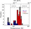 |
Fig. 9 Histogram of observed blackbody temperatures for all SEDs. Blackbody temperatures at ~6000 K (indicated in gray with a vertical line) very likely represent a detection of the host galaxy. A temperature of 30 000 K is indicated with another vertical gray line. |
Concerning the temperature, our results are consistent with what has been previously found (Zheng et al. 1997; Telfer et al. 2002; Scott et al. 2004; Binette et al. 2005; Shang et al. 2005). The temperature remains below ~32 000 K for all sources. Some BL Lac objects exhibit temperatures of ~6000 K (see Fig. 9, shown with a gray vertical line). Such cold blackbodies are very likely emission from the host galaxy, which would support the theory of a weak disk and inefficient accretion in BL Lac objects. Gravitational redshifting decreases the observed temperature, but even taking this effect into account would only slightly increase the temperatures by ~3000 K, which is still nowhere near the expected temperature for an accretion disk.
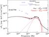 |
Fig. 10 Spectral energy distribution of the α state of 2142−758, with the best-fit single temperature blackbody (purple) and best-fit multitemperature accretion disk spectrum (red). |
In general, the spectral shape of the thermal excess is also inconsistent with an accretion disk origin. For all SEDs, the thermal excess can be described well by a single temperature blackbody. For an accretion disk extending from a few to several hundreds or thousands of gravitational radii a large range in temperature would be expected because of the r− 3/4 temperature profile of accretion disks with further slight stretching of the spectrum by gravitational redshifting. Figure 10 shows that the shape is reasonably constrained by Swift/UVOT. The red curve shows the spectrum expected from a simple multitemperature accretion disk. This diskbb model is not able to describe the narrow shape or a single temperature blackbody (purple line in Fig. 10). While this evidence is not conclusive owing to the low spectral resolution of the UVOT, it is nevertheless indicative of a more complex disk structure, which might be puffed up and warped or truncated, leading to changes in the thermal emission. Further theoretical and observational studies are necessary to determine the origin and shape of the BBB.
3.4. The black hole mass, MBH
We study how the properties of the SED depend on the black hole mass. The fundamental plane of black holes (Merloni et al. 2003; Gallo et al. 2003; Falcke et al. 2004; Körding et al. 2006; Gültekin et al. 2009, 2014; Plotkin et al. 2012; Bonchi et al. 2013; Saikia et al. 2015; Nisbet & Best 2016, and references therein) relates the radio and X-ray luminosity to the black hole mass, 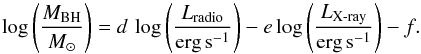 (3)The parameters d, e, and f depend on the source populations. Table 2 lists typical recent values for AGN. Here Lradio is the radio flux density measured at the frequency νradio listed in Table 2, while LX - ray is the X-ray flux in the 2−10 keV band. We caution that the radio luminosities listed are not “real” luminosities, as the differential flux at the given radio frequency is simply multiplied by
  , instead of using an integrated flux in a waveband.
Black hole mass measurements, based on measurements of the BBB (for FSRQs) and variability arguments (BL Lacs), only exist for 8 of the 20 sources in our sample and are taken from Ghisellini et al. (2010). We note that for some sources different black hole mass measurements exist (e.g., 0208−512; Stacy et al. 2003) that vary by an order of magnitude. We therefore use the fundamental plane to estimate the black hole mass and compare the estimates with measurements, where available. We use the distance-corrected radio flux density from the best-fit parabola model at the same frequency as used in each of the studies. The X-ray, 2–10 keV luminosity is taken from the separate fit to the X-ray data. We use all SEDs from this work and the corresponding X-ray and radio luminosities (where a redshift measurement is available, see Table 1) and calculated estimated black hole masses following Merloni et al. (2003), Körding et al. (2006), and Nisbet & Best (2016). Our results are presented in Table 3. For the results from Gültekin et al. (2009), we use Eq. (4) in their paper, with the parameters listed in Eq. (6), where a linear regression was performed to find an equation for an estimate of the black hole mass. For sources with more than one SED, the black hole mass estimates are averaged. The masses before averaging scatter depend on the source state with a maximum factor of 5 between the lowest and the highest estimate.
Black hole masses as measured and as estimated from the fundamental plane of black holes.
All estimates, except those using the parameters from Bonchi et al. (2013), are lower than the measured values, and the largest offset is that from the Merloni et al. (2003) parameters. Applying the relation by Bonchi et al. (2013) gives a very good agreement (less than a factor of 3) with the measurement values for several sources such as 0208−512, 0537−441, 1057−797, and 1454−354. The largest difference is seen between the measurement and estimate for 0447−439 with four orders of magnitude between the estimate using the Bonchi et al. (2013) parameters, and six orders of magnitude using the Merloni et al. (2003) parameters.
While a large scatter is observed for the fundamental plane (Nisbet & Best 2016), it probably does not explain a difference of four or six orders of magnitude. A possibility is that the relativistic boosting affects the observed masses in supermassive black holes, but not the Galactic black holes. However, this would imply that the intrinsic black hole masses in some of the AGN are much lower than previously believed. The uncertainties on the parameters of the fundamental plane are large; these are represented in the large uncertainties of the black hole mass estimates.
3.5. The strange SED of 2005−489
In general, all SEDs are described well by two log parabolas and a blackbody to describe the excess. A well-known VHE emitter, 2005−489 (Aharonian et al. 2005) is the only source with a strong deviation from this model. Piner & Edwards (2014) presented VLBI data of the source. The multiwavelength SED was studied several times (Kaufmann et al. 2009; H.E.S.S. Collaboration et al. 2010), with the H.E.S.S. Collaboration arguing about a hard, separate spectral component emerging in the X-ray observations in September 2005. This is in agreement with our results of the source during a high state. While over most of the energy range it shows a nonthermal parabolic behavior, its X-ray behavior in the high state (α) seems to be inconsistent with a leptonic model. In the low state (β), the photon index Γ = 2.28 ± 0.12 perfectly fits the parabolic shape; we note that the 104-month averaged BAT data point seems to indicate a small excess above a pure power law. While this is not conclusive, the photon index Γ = 1.70 ± 0.04 in the high state is inconsistent with the parabolic model (and a synchrotron model as well). The excess is reminiscent of a hadronic proton-synchrotron signature in the spectrum, while the LAT data might also show a dip in the spectrum, possibly due to a hadronic pion decay signature. While this evidence is not conclusive, it is the first source to show a clear deviation with a large difference in the photon index within a time span of less than two years. A caveat of this SED is the long time range over which the data were averaged in LAT, but it does not explain the change in index and the inconsistency between the Swift/UVOT and Swift/XRT data.
4. Summary and conclusions
We have studied a mainly γ-ray selected sample of southern blazars in the framework of the TANAMI project. We chose the 22 Fermi/LAT brightest sources from the TANAMI sample. This approach allowed us to use the LAT light curves with a Bayesian blocks algorithm to determine states of statistically constant flux. For time ranges with quasi-simultaneous data in the X-ray and radio band, we constructed broadband SEDs. We show that a “harder-when-brighter” trend is observed in the high state of the high-energy peak, shifting it to higher frequencies. The Compton dominance that we find is in agreement with previous results from the literature. When separated by source state, the Compton dominance in the high state shows a larger scatter and no discernible trend. We further study the bolometric Compton dominance using the integrated fluxes of peaks fit with parabolas. The scatter in this bolometric Compton dominance is lower, but it shows that the peak flux is a reliable tracer of the bolometric flux.
We study the temperature range and shape of the BBB. We find that the temperatures are consistent with previous results, showing temperatures that are too low for the expected accretion disk emission. It can possibly be explained by reprocessing the accretion disk emission by BLR clouds, which is also able to solve other problems. We also find that unexpectedly a single temperature model can best explain all BBBs, which is inconsistent with an accretion disk origin. It is unclear whether this is true for all blazars. No detailed model exists for a more realistic accretion disk that might be thick and/or warped. It is unclear how this would change the expected thermal emission.
We further study the fundamental plane of black holes as a tool for estimating black hole masses. We find that the parameters by Bonchi et al. (2013) for many sources are in good agreement with the black hole masses from Ghisellini et al. (2010), while this is not the case for other parameter estimates (those from Merloni et al. 2003; Körding et al. 2006; Gültekin et al. 2009; Nisbet & Best 2016), however the uncertainties are dominated by systematic effects and are very large. This shows that choosing the source population introduces selection effects. For a few sources, such as 0447−439, the measured mass is not in agreement with any of the parameters with a very large offset of greater than four orders of magnitude. We suggest that this might be due to boosting effects. This result would imply, however, that some AGN black hole masses are much lower than previously suspected.
Acknowledgments
We thank the referee for helpful comments. We thank S. Cutini for her useful comments. We thank S. Markoff for helpful discussions. We thank J. Perkins, L. Baldini, and S. Digel for carefully reading the manuscript. We thank M. Buxton for her help with the SMARTS data. We acknowledge support and partial funding by the Deutsche Forschungsgemeinschaft grant WI 1860-10/1 (TANAMI) and GRK 1147, Deutsches Zentrum für Luft- und Raumfahrt grants 50 OR 1311 and 50 OR 1103, and the Helmholtz Alliance for Astroparticle Physics (HAP). This research was funded in part by NASA through Fermi Guest Investigator grants NNH09ZDA001N, NH10ZDA001N, NNH12ZDA001N, and NNH13ZDA001N-FERMI. This research was supported by an appointment to the NASA Postdoctoral Program at the Goddard Space Flight Center, administered by Oak Ridge Associated Universities through a contract with NASA. E.R. was partially supported by the Spanish MINECO project AYA2012-38491-C02-01 and by the Generalitat Valenciana project PROMETEO II/2014/057. We thank J. E. Davis for the development of the slxfig module that was used to prepare the figures in this work. We thank T. Johnson for the Fermi/LAT SED scripts, which were used to calculate the Fermi/LAT spectra. This research has made use of a collection of ISIS scripts provided by the Dr. Karl Remeis-Observatory, Bamberg, Germany at http://www.sternwarte.uni-erlangen.de/isis/. The Long Baseline Array and Australia Telescope Compact Array are part of the Australia Telescope National Facility, which is funded by the Commonwealth of Australia for operation as a National Facility managed by CSIRO.
This paper has made use of up-to-date SMARTS optical/near-infrared light curves that are available at www.astro.yale.edu/smarts/glast/home.php.
The Fermi LAT Collaboration acknowledges generous ongoing support from a number of agencies and institutes that have supported both the development and the operation of the LAT as well as scientific data analysis. These include the National Aeronautics and Space Administration and the Department of Energy in the United States, the Commissariat à l’Energie Atomique and the Centre National de la Recherche Scientifique/Institut National de Physique Nucléaire et de Physique des Particules in France, the Agenzia Spaziale Italiana and the Istituto Nazionale di Fisica Nucleare in Italy, the Ministry of Education, Culture, Sports, Science and Technology (MEXT), High Energy Accelerator Research Organization (KEK) and Japan Aerospace Exploration Agency (JAXA) in Japan, and the K.A. Wallenberg Foundation, the Swedish Research Council and the Swedish National Space Board in Sweden. Additional support for science analysis during the operations phase is gratefully acknowledged from the Istituto Nazionale di Astrofisica in Italy and the Centre National d’Études Spatiales in France.
References
- Abdo, A. A., Ackermann, M., Ajello, M., et al. 2009, ApJ, 699, 817 [NASA ADS] [CrossRef] [Google Scholar]
- Abdo, A. A., Ackermann, M., Agudo, I., et al. 2010a, ApJ, 716, 30 [NASA ADS] [CrossRef] [Google Scholar]
- Abdo, A. A., Ackermann, M., Ajello, M., et al. 2011a, ApJ, 730, 101 [NASA ADS] [CrossRef] [Google Scholar]
- Abdo, A. A., Ackermann, M., Ajello, M., et al. 2010b, ApJ, 722, 520 [NASA ADS] [CrossRef] [Google Scholar]
- Abdo, A. A., Ackermann, M., Ajello, M., et al. 2010c, ApJ, 710, 1271 [NASA ADS] [CrossRef] [Google Scholar]
- Abdo, A. A., Ackermann, M., Ajello, M., et al. 2010d, ApJ, 710, 810 [NASA ADS] [CrossRef] [Google Scholar]
- Abdo, A. A., Ackermann, M., Ajello, M., et al. 2011b, ApJ, 736, 131 [NASA ADS] [CrossRef] [Google Scholar]
- Acero, F., Ackermann, M., Ajello, M., et al. 2015, ApJS, 218, 23 [Google Scholar]
- Ackermann, M., Ajello, M., Albert, A., et al. 2012, ApJS, 203, 4 [NASA ADS] [CrossRef] [Google Scholar]
- Ackermann, M., Ajello, M., Atwood, W. B., et al. 2015, ApJ, 810, 14 [NASA ADS] [CrossRef] [Google Scholar]
- Aharonian, F., Akhperjanian, A. G., Aye, K.-M., et al. 2005, A&A, 436, L17 [NASA ADS] [CrossRef] [EDP Sciences] [Google Scholar]
- Aharonian, F., Akhperjanian, A. G., Anton, G., et al. 2009, ApJ, 696, L150 [NASA ADS] [CrossRef] [Google Scholar]
- Aleksić, J., Antonelli, L. A., Antoranz, P., et al. 2013, A&A, 556, A67 [NASA ADS] [CrossRef] [EDP Sciences] [Google Scholar]
- Aleksić, J., Ansoldi, S., Antonelli, L. A., et al. 2015, A&A, 573, A50 [NASA ADS] [CrossRef] [EDP Sciences] [Google Scholar]
- Antonucci, R. 1993, ARA&A, 31, 473 [Google Scholar]
- Antonucci, R. 2002, in Astrophysical Spectropolarimetry. XII Canary Islands Winter School of Astrophysics, Puerto de la Cruz, Tenerife, Spain, eds. J. Trujillo-Bueno, F. Moreno-Insertis, & F. Sánchez, 151 [Google Scholar]
- Atwood, W. B., Abdo, A. A., Ackermann, M., et al. 2009, ApJ, 697, 1071 [NASA ADS] [CrossRef] [Google Scholar]
- Avni, Y., & Tananbaum, H. 1982, ApJ, 262, L17 [NASA ADS] [CrossRef] [Google Scholar]
- Bajaja, E., Arnal, E. M., Larrarte, J. J., et al. 2005, A&A, 440, 767 [NASA ADS] [CrossRef] [EDP Sciences] [Google Scholar]
- Baloković, M., Paneque, D., Madejski, G., et al. 2016, ApJ, 819, 156 [NASA ADS] [CrossRef] [Google Scholar]
- Bartoli, B., Bernardini, P., Bi, X. J., et al. 2012, ApJ, 758, 2 [NASA ADS] [CrossRef] [Google Scholar]
- Bartoli, B., Bernardini, P., Bi, X. J., et al. 2016, ApJS, 222, 6 [NASA ADS] [CrossRef] [Google Scholar]
- Barvainis, R. 1993, ApJ, 412, 513 [NASA ADS] [CrossRef] [Google Scholar]
- Baumgartner, W. H., Tueller, J., Markwardt, C. B., et al. 2013, ApJS, 207, 19 [NASA ADS] [CrossRef] [EDP Sciences] [Google Scholar]
- Beasley, A. J., Gordon, D., Peck, A. B., et al. 2002, ApJS, 141, 13 [NASA ADS] [CrossRef] [Google Scholar]
- Beringer, J., Arguin, J.-F., Barnett, R. M., et al. 2012, Phys. Rev. D, 86, 010001 [Google Scholar]
- Bessell, M. S., Castelli, F., & Plez, B. 1998, A&A, 333, 231 [NASA ADS] [Google Scholar]
- Binette, L., Magris, C. G., Krongold, Y., et al. 2005, ApJ, 631, 661 [NASA ADS] [CrossRef] [Google Scholar]
- Blanchard, J. M. 2013, Ph.D. Thesis, Univ. Tasmania Australia [Google Scholar]
- Blandford, R. D., & Rees, M. J. 1978, in BL Lac Objects, ed. A. M. Wolfe (Univ. Pittsburgh Press), 328 [Google Scholar]
- Błażejowski, M., Blaylock, G., Bond, I. H., et al. 2005, ApJ, 630, 130 [NASA ADS] [CrossRef] [Google Scholar]
- Böck, M., Kadler, M., Müller, C., et al. 2016, A&A, 590, A40 [NASA ADS] [CrossRef] [EDP Sciences] [Google Scholar]
- Bonchi, A., La Franca, F., Melini, G., Bongiorno, A., & Fiore, F. 2013, MNRAS, 429, 1970 [NASA ADS] [CrossRef] [Google Scholar]
- Bonning, E., Urry, C. M., Bailyn, C., et al. 2012, ApJ, 756, 13 [NASA ADS] [CrossRef] [Google Scholar]
- Böttcher, M., Reimer, A., & Marscher, A. P. 2009, ApJ, 703, 1168 [NASA ADS] [CrossRef] [Google Scholar]
- Böttcher, M., Reimer, A., Sweeney, K., & Prakash, A. 2013, ApJ, 768, 54 [NASA ADS] [CrossRef] [Google Scholar]
- Breeveld, A. A., Curran, P. A., Hoversten, E. A., et al. 2010, MNRAS, 406, 1687 [NASA ADS] [Google Scholar]
- Breeveld, A. A., Poole, T. S., James, C. H., et al. 2005, in UV, X-Ray, and Gamma-Ray Space Instrumentation for Astronomy XIV, ed. O. H. W. Siegmund, SPIE Conf. Ser., 5898, 391 [Google Scholar]
- Breeveld, A. A., Landsman, W., Holland, S. T., et al. 2011, in AIP Conf. Ser. 1358, eds. J. E. McEnery, J. L. Racusin, & N. Gehrels, 373 [Google Scholar]
- Broos, P. S., Townsley, L. K., Feigelson, E. D., et al. 2010, ApJ, 714, 1582 [NASA ADS] [CrossRef] [Google Scholar]
- Browne, I. W. A., Savage, A., & Bolton, J. G. 1975, MNRAS, 173, 87P [NASA ADS] [Google Scholar]
- Buxton, M. M., Bailyn, C. D., Capelo, H. L., et al. 2012, AJ, 143, 130 [NASA ADS] [CrossRef] [Google Scholar]
- Carnerero, M. I., Raiteri, C. M., Villata, M., et al. 2015, MNRAS, 450, 2677 [NASA ADS] [CrossRef] [Google Scholar]
- Chandra, S., Zhang, H., Kushwaha, P., et al. 2015, ApJ, 809, 130 [NASA ADS] [CrossRef] [Google Scholar]
- Craig, N., & Fruscione, A. 1997, AJ, 114, 1356 [NASA ADS] [CrossRef] [Google Scholar]
- D’Ammando, F., Antolini, E., Tosti, G., et al. 2013, MNRAS, 431, 2481 [NASA ADS] [CrossRef] [Google Scholar]
- D’Ammando, F., Orienti, M., Tavecchio, F., et al. 2015, MNRAS, 450, 3975 [NASA ADS] [CrossRef] [Google Scholar]
- Donnarumma, I., Vittorini, V., Vercellone, S., et al. 2009, ApJ, 691, L13 [NASA ADS] [CrossRef] [Google Scholar]
- Dutka, M. S., Ojha, R., Pottschmidt, K., et al. 2013, ApJ, 779, 174 [NASA ADS] [CrossRef] [Google Scholar]
- Elias, J. H., Frogel, J. A., Matthews, K., & Neugebauer, G. 1982, AJ, 87, 1029 [NASA ADS] [CrossRef] [Google Scholar]
- Elvis, M., Wilkes, B. J., McDowell, J. C., et al. 1994, ApJS, 95, 1 [NASA ADS] [CrossRef] [Google Scholar]
- Emmanoulopoulos, D., Papadakis, I. E., McHardy, I. M., et al. 2012, MNRAS, 424, 1327 [NASA ADS] [CrossRef] [Google Scholar]
- Falcke, H., Körding, E., & Markoff, S. 2004, A&A, 414, 895 [NASA ADS] [CrossRef] [EDP Sciences] [Google Scholar]
- Falomo, R., Maraschi, L., Treves, A., & Tanzi, E. G. 1987, ApJ, 318, L39 [NASA ADS] [CrossRef] [Google Scholar]
- Falomo, R., Pesce, J. E., & Treves, A. 1993, ApJ, 411, L63 [NASA ADS] [CrossRef] [Google Scholar]
- Fey, A. L., Ma, C., Arias, E. F., et al. 2004, AJ, 127, 3587 [NASA ADS] [CrossRef] [Google Scholar]
- Fey, A. L., Ojha, R., Quick, J. F. H., et al. 2006, AJ, 132, 1944 [NASA ADS] [CrossRef] [Google Scholar]
- Finke, J. D. 2013, ApJ, 763, 134 [NASA ADS] [CrossRef] [Google Scholar]
- Finke, J. D., Dermer, C. D., & Böttcher, M. 2008, ApJ, 686, 181 [NASA ADS] [CrossRef] [Google Scholar]
- Fossati, G., Maraschi, L., Celotti, A., Comastri, A., & Ghisellini, G. 1998, MNRAS, 299, 433 [NASA ADS] [CrossRef] [Google Scholar]
- Frogel, J. A., Persson, S. E., Matthews, K., & Aaronson, M. 1978, ApJ, 220, 75 [NASA ADS] [CrossRef] [Google Scholar]
- Furniss, A., Noda, K., Boggs, S., et al. 2015, ApJ, 812, 65 [NASA ADS] [CrossRef] [Google Scholar]
- Gallo, E., Fender, R. P., & Pooley, G. G. 2003, MNRAS, 344, 60 [NASA ADS] [CrossRef] [Google Scholar]
- Gehrels, N., Chincarini, G., Giommi, P., et al. 2004, ApJ, 611, 1005 [NASA ADS] [CrossRef] [Google Scholar]
- Getman, K. V., Feigelson, E. D., Broos, P. S., Townsley, L. K., & Garmire, G. P. 2010, ApJ, 708, 1760 [NASA ADS] [CrossRef] [Google Scholar]
- Ghisellini, G. 2013, in The Innermost Regions of Relativistic Jets and Their Magnetic Fields, Granada, Spain, EPJ Web Conf., 61, 5001 [CrossRef] [EDP Sciences] [Google Scholar]
- Ghisellini, G., Celotti, A., Fossati, G., Maraschi, L., & Comastri, A. 1998, MNRAS, 301, 451 [NASA ADS] [CrossRef] [Google Scholar]
- Ghisellini, G., Maraschi, L., & Tavecchio, F. 2009, MNRAS, 396, L105 [NASA ADS] [Google Scholar]
- Ghisellini, G., Tavecchio, F., Foschini, L., et al. 2010, MNRAS, 402, 497 [NASA ADS] [CrossRef] [Google Scholar]
- Giommi, P., Ansari, S. G., & Micol, A. 1995, A&ASS, 109, 267 [NASA ADS] [Google Scholar]
- Giommi, P., Capalbi, M., Fiocchi, M., et al. 2002, in Blazar Astrophysics with BeppoSAX and Other Observatories, eds. P. Giommi, E. Massaro, & G. Palumbo, Proc. of workshop, ASI Sp. Publ., 63 [Google Scholar]
- Giommi, P., Blustin, A. J., Capalbi, M., et al. 2006, A&A, 456, 911 [NASA ADS] [CrossRef] [EDP Sciences] [Google Scholar]
- Giommi, P., Padovani, P., Polenta, G., et al. 2012a, MNRAS, 420, 2899 [NASA ADS] [CrossRef] [Google Scholar]
- Giommi, P., Polenta, G., Lähteenmäki, A., et al. 2012b, A&A, 541, A160 [NASA ADS] [CrossRef] [EDP Sciences] [Google Scholar]
- Grandi, P., Urry, C. M., Maraschi, L., et al. 1996, ApJ, 459, 73 [NASA ADS] [CrossRef] [Google Scholar]
- Gültekin, K., Cackett, E. M., Miller, J. M., et al. 2009, ApJ, 706, 404 [NASA ADS] [CrossRef] [Google Scholar]
- Gültekin, K., Cackett, E. M., King, A. L., Miller, J. M., & Pinkney, J. 2014, ApJ, 788, L22 [NASA ADS] [CrossRef] [Google Scholar]
- Hayashida, M., Nalewajko, K., Madejski, G. M., et al. 2015, ApJ, 807, 79 [Google Scholar]
- Healey, S. E., Romani, R. W., Taylor, G. B., et al. 2007, ApJS, 171, 61 [NASA ADS] [CrossRef] [Google Scholar]
- Healey, S. E., Romani, R. W., Cotter, G., et al. 2008, ApJS, 175, 97 [NASA ADS] [CrossRef] [Google Scholar]
- Heidt, J., Tröller, M., Nilsson, K., et al. 2004, A&A, 418, 813 [NASA ADS] [CrossRef] [EDP Sciences] [Google Scholar]
- H.E.S.S. Collaboration, Acero, F., Aharonian, F., et al. 2010, A&A, 511, A52 [NASA ADS] [CrossRef] [EDP Sciences] [Google Scholar]
- Hewitt, A., & Burbidge, G. 1987, ApJS, 63, 1 [NASA ADS] [CrossRef] [Google Scholar]
- Houck, J. C., & Denicola, L. A. 2000, in Astronomical Data Analysis Software and Systems IX, eds. N. Manset, C. Veillet, & D. Crabtree, ASP Conf. Ser., 216, 591 [Google Scholar]
- Hunstead, R. W., & Murdoch, H. S. 1980, MNRAS, 192, 31P [NASA ADS] [Google Scholar]
- Hunstead, R. W., Murdoch, H. S., & Shobbrook, R. R. 1978, MNRAS, 185, 149 [NASA ADS] [Google Scholar]
- Impey, C. D., & Tapia, S. 1988, ApJ, 333, 666 [NASA ADS] [CrossRef] [Google Scholar]
- Jackson, C. A., Wall, J. V., Shaver, P. A., et al. 2002, A&A, 386, 97 [NASA ADS] [CrossRef] [EDP Sciences] [Google Scholar]
- Jauncey, D. L., Batty, M. J., Wright, A. E., Peterson, B. A., & Savage, A. 1984, ApJ, 286, 498 [NASA ADS] [CrossRef] [Google Scholar]
- Johnston, K. J., Fey, A. L., Zacharias, N., et al. 1995, AJ, 110, 880 [NASA ADS] [CrossRef] [Google Scholar]
- Jolley, E. J. D., Kuncic, Z., Bicknell, G. V., & Wagner, S. 2009, MNRAS, 400, 1521 [NASA ADS] [CrossRef] [Google Scholar]
- Jones, D. H., Saunders, W., Colless, M., et al. 2004, MNRAS, 355, 747 [NASA ADS] [CrossRef] [Google Scholar]
- Jones, D. H., Read, M. A., Saunders, W., et al. 2009, MNRAS, 399, 683 [NASA ADS] [CrossRef] [Google Scholar]
- Kadler, M., Ojha, R., & TANAMI Collaboration. 2015, Astron. Nachr., 336, 499 [NASA ADS] [CrossRef] [Google Scholar]
- Kalberla, P. M. W., Burton, W. B., Hartmann, D., et al. 2005, A&A, 440, 775 [NASA ADS] [CrossRef] [EDP Sciences] [Google Scholar]
- Kaufmann, S., Hauser, M., Kosack, K., et al. 2009, in 2009 Fermi Symposium, eConf. Proc. C091122 [Google Scholar]
- Körding, E., Falcke, H., & Corbel, S. 2006, A&A, 456, 439 [NASA ADS] [CrossRef] [EDP Sciences] [Google Scholar]
- Lampton, M., Margon, B., & Bowyer, S. 1976, ApJ, 208, 177 [NASA ADS] [CrossRef] [Google Scholar]
- Lawrence, A. 2012, MNRAS, 423, 451 [NASA ADS] [CrossRef] [Google Scholar]
- Liao, N. H., Bai, J. M., Liu, H. T., et al. 2014, ApJ, 783, 83 [NASA ADS] [CrossRef] [Google Scholar]
- Ma, C., Arias, E. F., Eubanks, T. M., et al. 1998, AJ, 116, 516 [NASA ADS] [CrossRef] [Google Scholar]
- Maitra, D., Miller, J. M., Markoff, S., & King, A. 2011, ApJ, 735, 107 [NASA ADS] [CrossRef] [Google Scholar]
- Makishima, K., Maejima, Y., Mitsuda, K., et al. 1986, ApJ, 308, 635 [NASA ADS] [CrossRef] [Google Scholar]
- Malkan, M. A., & Sargent, W. L. W. 1982, ApJ, 254, 22 [NASA ADS] [CrossRef] [Google Scholar]
- Mannheim, K. 1993, A&A, 269, 67 [NASA ADS] [Google Scholar]
- Mannheim, K., & Biermann, P. L. 1992, A&A, 253, L21 [NASA ADS] [Google Scholar]
- Marscher, A. P., Jorstad, S. G., Larionov, V. M., et al. 2010, ApJ, 710, L126 [NASA ADS] [CrossRef] [Google Scholar]
- Massaro, E., Perri, M., Giommi, P., & Nesci, R. 2004, A&A, 413, 489 [NASA ADS] [CrossRef] [EDP Sciences] [Google Scholar]
- Massaro, E., Giommi, P., Leto, C., et al. 2009, A&A, 495, 691 [NASA ADS] [CrossRef] [EDP Sciences] [Google Scholar]
- McCulloch, P. M., Ellingsen, S. P., Jauncey, D. L., et al. 2005, AJ, 129, 2034 [NASA ADS] [CrossRef] [Google Scholar]
- Merloni, A., Heinz, S., & di Matteo, T. 2003, MNRAS, 345, 1057 [NASA ADS] [CrossRef] [Google Scholar]
- Meyer, E. T., Fossati, G., Georganopoulos, M., & Lister, M. L. 2011, ApJ, 740, 98 [NASA ADS] [CrossRef] [Google Scholar]
- Mitsuda, K., Inoue, H., Koyama, K., et al. 1984, PASJ, 36, 741 [NASA ADS] [Google Scholar]
- Nieppola, E., Tornikoski, M., & Valtaoja, E. 2006, A&A, 445, 441 [NASA ADS] [CrossRef] [EDP Sciences] [Google Scholar]
- Nisbet, D. M., & Best, P. N. 2016, MNRAS, 455, 2551 [NASA ADS] [CrossRef] [Google Scholar]
- Nowak, M. A., Wilms, J., Heinz, S., et al. 2005, ApJ, 626, 1006 [NASA ADS] [CrossRef] [Google Scholar]
- Nowak, M. A., Neilsen, J., Markoff, S. B., et al. 2012, ApJ, 759, 95 [NASA ADS] [CrossRef] [Google Scholar]
- Ojha, R., Kadler, M., Böck, M., et al. 2010, A&A, 519, A45 [NASA ADS] [CrossRef] [EDP Sciences] [Google Scholar]
- Pacciani, L., Vittorini, V., Tavani, M., et al. 2010, ApJ, 716, L170 [NASA ADS] [CrossRef] [Google Scholar]
- Padovani, P., & Giommi, P. 1995, ApJ, 444, 567 [NASA ADS] [CrossRef] [Google Scholar]
- Padovani, P., Giommi, P., Ábrahám, P., Csizmadia, S., & Moór, A. 2006, A&A, 456, 131 [NASA ADS] [CrossRef] [EDP Sciences] [Google Scholar]
- Paliya, V. S., Sahayanathan, S., & Stalin, C. S. 2015, ApJ, 803, 15 [NASA ADS] [CrossRef] [Google Scholar]
- Persson, S. E., Murphy, D. C., Krzeminski, W., Roth, M., & Rieke, M. J. 1998, AJ, 116, 2475 [NASA ADS] [CrossRef] [Google Scholar]
- Peterson, B. A., Jauncey, D. L., Condon, J. J., & Wright, A. E. 1976, ApJ, 207, L5 [NASA ADS] [CrossRef] [Google Scholar]
- Pian, E., Vacanti, G., Tagliaferri, G., et al. 1998, ApJ, 492, L17 [NASA ADS] [CrossRef] [Google Scholar]
- Piner, B. G., & Edwards, P. G. 2014, ApJ, 797, 25 [NASA ADS] [CrossRef] [Google Scholar]
- Planck Collaboration XXVIII. 2014, A&A, 571, A28 [NASA ADS] [CrossRef] [EDP Sciences] [Google Scholar]
- Plotkin, R. M., Markoff, S., Kelly, B. C., Körding, E., & Anderson, S. F. 2012, MNRAS, 419, 267 [NASA ADS] [CrossRef] [Google Scholar]
- Poole, T. S., Breeveld, A. A., Page, M. J., et al. 2008, MNRAS, 383, 627 [NASA ADS] [CrossRef] [Google Scholar]
- Predehl, P., & Schmitt, J. H. M. M. 1995, A&A, 293, 889 [NASA ADS] [Google Scholar]
- Rani, B., Krichbaum, T. P., Fuhrmann, L., et al. 2013, A&A, 552, A11 [NASA ADS] [CrossRef] [EDP Sciences] [Google Scholar]
- Romano, P., Cusumano, G., Campana, S., et al. 2005, in UV, X-Ray, and Gamma-Ray Space Instrumentation for Astronomy XIV, ed. O. H. W. Siegmund, SPIE Conf. Ser., 5898, 369 [Google Scholar]
- Saikia, P., Körding, E., & Falcke, H. 2015, MNRAS, 450, 2317 [NASA ADS] [CrossRef] [Google Scholar]
- Sambruna, R. M., Maraschi, L., & Urry, C. M. 1996, ApJ, 463, 444 [NASA ADS] [CrossRef] [Google Scholar]
- Sanders, D. B., Phinney, E. S., Neugebauer, G., Soifer, B. T., & Matthews, K. 1989, ApJ, 347, 29 [NASA ADS] [CrossRef] [Google Scholar]
- Sbarufatti, B., Ciprini, S., Kotilainen, J., et al. 2009, AJ, 137, 337 [NASA ADS] [CrossRef] [Google Scholar]
- Scargle, J. D. 1998, ApJ, 504, 405 [NASA ADS] [CrossRef] [Google Scholar]
- Scargle, J. D., Norris, J. P., Jackson, B., & Chiang, J. 2013, ApJ, 764, 167 [NASA ADS] [CrossRef] [Google Scholar]
- Scott, J. E., Kriss, G. A., Brotherton, M., et al. 2004, ApJ, 615, 135 [NASA ADS] [CrossRef] [Google Scholar]
- Shang, Z., Brotherton, M. S., Green, R. F., et al. 2005, ApJ, 619, 41 [NASA ADS] [CrossRef] [Google Scholar]
- Shaw, M. S., Romani, R. W., Cotter, G., et al. 2012, ApJ, 748, 49 [CrossRef] [Google Scholar]
- Shen, Z.-Q., Wan, T.-S., Moran, J. M., et al. 1998, AJ, 115, 1357 [NASA ADS] [CrossRef] [Google Scholar]
- Shields, G. A. 1978, Nature, 272, 706 [NASA ADS] [CrossRef] [Google Scholar]
- Sikora, M., Begelman, M. C., & Rees, M. J. 1994, ApJ, 421, 153 [NASA ADS] [CrossRef] [Google Scholar]
- Sikora, M., Stawarz, Ł., Moderski, R., Nalewajko, K., & Madejski, G. M. 2009, ApJ, 704, 38 [NASA ADS] [CrossRef] [Google Scholar]
- Sitko, M. L., & Junkkarinen, V. T. 1985, PASP, 97, 1158 [NASA ADS] [CrossRef] [Google Scholar]
- Skrutskie, M. F., Cutri, R. M., Stiening, R., et al. 2006, AJ, 131, 1163 [NASA ADS] [CrossRef] [Google Scholar]
- Soldi, S., Türler, M., Paltani, S., et al. 2008, A&A, 486, 411 [NASA ADS] [CrossRef] [EDP Sciences] [Google Scholar]
- Stacy, J. G., Vestrand, W. T., & Sreekumar, P. 2003, ApJ, 598, 216 [NASA ADS] [CrossRef] [Google Scholar]
- Stevens, J., Edwards, P. G., Ojha, R., et al. 2012, in 2012 Fermi & Jansky Proc.: Our Evolving Understanding of AGN, eConf. Proc. C1111101 [Google Scholar]
- Strüder, L., Briel, U., Dennerl, K., et al. 2001, A&A, 365, L18 [NASA ADS] [CrossRef] [EDP Sciences] [Google Scholar]
- Tagliaferri, G., Ghisellini, G., Perri, M., et al. 2015, ApJ, 807, 167 [NASA ADS] [CrossRef] [Google Scholar]
- Tanaka, Y. T., Stawarz, Ł., Thompson, D. J., et al. 2011, ApJ, 733, 19 [NASA ADS] [CrossRef] [Google Scholar]
- Telfer, R. C., Zheng, W., Kriss, G. A., & Davidsen, A. F. 2002, ApJ, 565, 773 [NASA ADS] [CrossRef] [Google Scholar]
- Türler, M., Paltani, S., Courvoisier, T. J.-L., et al. 1999, A&AS, 134, 89 [NASA ADS] [CrossRef] [EDP Sciences] [Google Scholar]
- Turner, M. J. L., Abbey, A., Arnaud, M., et al. 2001, A&A, 365, L27 [NASA ADS] [CrossRef] [EDP Sciences] [Google Scholar]
- Urry, C. M., & Padovani, P. 1995, PASP, 107, 803 [NASA ADS] [CrossRef] [Google Scholar]
- Valtaoja, E., Lähteenmäki, A., Teräsranta, H., & Lainela, M. 1999, ApJS, 120, 95 [NASA ADS] [CrossRef] [Google Scholar]
- Vercellone, S., Chen, A. W., Vittorini, V., et al. 2009, ApJ, 690, 1018 [NASA ADS] [CrossRef] [Google Scholar]
- Vermeulen, R. C., Ogle, P. M., Tran, H. D., et al. 1995, ApJ, 452, L5 [NASA ADS] [CrossRef] [Google Scholar]
- Véron-Cetty, M.-P., & Véron, P. 2006, A&A, 455, 773 [NASA ADS] [CrossRef] [EDP Sciences] [Google Scholar]
- Vignali, C., Brandt, W. N., & Schneider, D. P. 2003, AJ, 125, 433 [NASA ADS] [CrossRef] [Google Scholar]
- von Montigny, C., Bertsch, D. L., Chiang, J., et al. 1995, ApJ, 440, 525 [NASA ADS] [CrossRef] [Google Scholar]
- Walter, R., Rohlfs, R., Meharga, M. T., et al. 2010, PoS(INTEGRAL 2010)162 [Google Scholar]
- Wehrle, A. E., Pian, E., Urry, C. M., et al. 1998, ApJ, 497, 178 [NASA ADS] [CrossRef] [Google Scholar]
- Wehrle, A. E., Grupe, D., Jorstad, S. G., et al. 2016, ApJ, 816, 53 [NASA ADS] [CrossRef] [Google Scholar]
- Weidinger, M., & Spanier, F. 2015, A&A, 573, A7 [NASA ADS] [CrossRef] [EDP Sciences] [Google Scholar]
- White, G. L., Jauncey, D. L., Wright, A. E., et al. 1988, ApJ, 327, 561 [NASA ADS] [CrossRef] [Google Scholar]
- Winkler, C., Courvoisier, T. J.-L., Di Cocco, G., et al. 2003, A&A, 411, L1 [NASA ADS] [CrossRef] [EDP Sciences] [Google Scholar]
- Wisotzki, L., Christlieb, N., Bade, N., et al. 2000, A&A, 358, 77 [NASA ADS] [Google Scholar]
- Wright, E. L., Eisenhardt, P. R. M., Mainzer, A. K., et al. 2010, AJ, 140, 1868 [NASA ADS] [CrossRef] [Google Scholar]
- Zamorani, G., Henry, J. P., Maccacaro, T., et al. 1981, ApJ, 245, 357 [NASA ADS] [CrossRef] [Google Scholar]
- Zheng, W., Kriss, G. A., Telfer, R. C., Grimes, J. P., & Davidsen, A. F. 1997, ApJ, 475, 469 [NASA ADS] [CrossRef] [Google Scholar]
Appendix A: Results: Light curves and SEDs
Appendix A.1: Fermi/LAT light curves
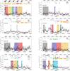 |
Fig. A.1 Fermi/LAT light curves for all sources with a known redshift, from August 4, 2008 up to January 1, 2015. A Bayesian blocks analysis was performed on the data and is shown in dark gray. The horizontal pink line shows the average flux over the full light curve. Observations by Swift, XMM-Newton, REM, SMARTS, Ceduna, ATCA, or VLBI are indicated with a line at the corresponding time. Blocks with sufficient data for a broadband SED are shown in color and labeled with Greek letters. The colors correspond to the colors used in the broadband spectra. |
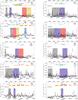 |
Fig. A.1 continued. |
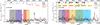 |
Fig. A.1 continued. |
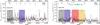 |
Fig. A.2 Fermi/LAT light curves for both sources without a known redshift, from August 4, 2008 up to 2015 January 1. A Bayesian blocks analysis was performed on the data and is shown in dark gray. The horizontal pink line shows the average flux over the full light curve. Observations by Swift, REM, Ceduna, and VLBI are indicated with a line at the corresponding time. Blocks with sufficient data for a broadband SED are shown in color and labeled with Greek letters. The colors correspond to the colors used in the broadband spectra. |
Appendix A.2: Broadband spectral energy distributions
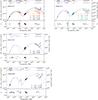 |
Fig. A.3 Broadband spectral energy distributions of all sources with a redshift in the log log νFν representation. For sources with more than 3 states with sufficient data, the plots were split into two parts to ensure that the SEDs are easily visible. Fit models are shown in dashed lines if archival data had to be included in the fit. For sources with a thermal excess in the optical/UV, a blackbody was included (dotted). The instruments (including their spectral range) are shown above the spectrum. The colors correspond to the colors used in the light curve. The best -fit reduced χ2 value is shown at the bottom right for every state. Residuals are shown in the lower panel. The spectra have not been k-corrected. |
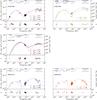 |
Fig. A.3 continued. |
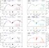 |
Fig. A.3 continued. |
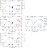 |
Fig. A.3 continued. |
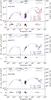 |
Fig. A.3 continued. |
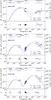 |
Fig. A.3 continued. |
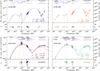 |
Fig. A.3 continued. |
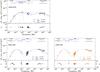 |
Fig. A.4 Broadband spectral energy distributions for both sources without a redshift in the log log νFν representation. For sources with more than 3 states with sufficient data, the plots were split into two parts to ensure that the SEDs are easily visible. Fit models are shown in dashed lines if archival data had to be included in the fit. For sources with a thermal excess in the optical/UV, a blackbody was included (dotted). The instruments (including their spectral range) are shown above the spectrum. The colors correspond to the colors used in the light curve. The best-fit reduced χ2 value is shown at the bottom right for every state. Residuals are shown in the lower panel. The spectra have not been k-corrected. |
Appendix A.3: Fit results
Fit results for all individual SEDs, listed by source and state.
continued.
All Tables
Black hole masses as measured and as estimated from the fundamental plane of black holes.
All Figures
|
Fig. 1 Broadband spectral model of 0402−362 with two logarithmic parabolas including reddening and absorption (blue), a dereddened and reddened blackbody (red, red dashed), and the total unabsorbed model (black). |
| In the text | |
|
Fig. 2 Peak frequency (k-corrected) and peak luminosity for the synchrotron peak (left) and the high-energy peak (right). The estimated uncertainty is given in the lower left corner for sources with average coverage (orange) and for SEDs with a lack of data near the peak position (gray). |
| In the text | |
|
Fig. 3 “Inverted blazar sequence”: HE peak luminosity (left) vs. peak synchrotron frequency (k-corrected) and vice versa (right). The estimated uncertainty is given in the lower left corner for sources with average coverage (orange) and for SEDs with a lack of data near the peak position (gray). |
| In the text | |
|
Fig. 4 Peak frequencies and peak luminosities, separated into low, intermediate, and high states for the synchrotron peak (top row) and high-energy peak (bottom row). While the low and intermediate states follow the blazar sequence for both peaks, the high-energy peak in both states show a peculiar, almost inverted behavior, although the number of sources (especially BL Lacertae objects) is too low for any conclusive evidence. The estimated uncertainty is given in the lower left corner of the left panels for sources with average coverage (orange) and for SEDs with a lack of data near the peak position (gray). |
| In the text | |
|
Fig. 5 Behavior of the synchrotron (left) and HE (right) peak frequency as a function of the photon index seen in the Fermi/LAT (top) and Swift/XRT bands (bottom). |
| In the text | |
|
Fig. 6 Synchrotron (top) and HE (bottom) peak frequency vs. the photon index seen by Swift/XRT (top) and Fermi/LAT (bottom) separated by low, intermediate, and high states. |
| In the text | |
|
Fig. 7 Top left: Compton dominance for all SEDs for all sources (no k-correction). The blazars’ divide is particularly strong; only few sources are found between 1014 and 1015 Hz. Top right and bottom: same as above, but SEDs are separated into low, intermediate, and high states. The estimated uncertainty is given in the lower left corner of the top right panel in gray. |
| In the text | |
|
Fig. 8 Top left: bolometric Compton dominance for all SEDs for all sources (no k-correction). The blazars’ divide is particularly strong. Top right and bottom: same as above, but SEDs are separated into low, intermediate, and high states. The estimated uncertainty is given in the lower left corner of the top right panel in gray. |
| In the text | |
|
Fig. 9 Histogram of observed blackbody temperatures for all SEDs. Blackbody temperatures at ~6000 K (indicated in gray with a vertical line) very likely represent a detection of the host galaxy. A temperature of 30 000 K is indicated with another vertical gray line. |
| In the text | |
|
Fig. 10 Spectral energy distribution of the α state of 2142−758, with the best-fit single temperature blackbody (purple) and best-fit multitemperature accretion disk spectrum (red). |
| In the text | |
|
Fig. A.1 Fermi/LAT light curves for all sources with a known redshift, from August 4, 2008 up to January 1, 2015. A Bayesian blocks analysis was performed on the data and is shown in dark gray. The horizontal pink line shows the average flux over the full light curve. Observations by Swift, XMM-Newton, REM, SMARTS, Ceduna, ATCA, or VLBI are indicated with a line at the corresponding time. Blocks with sufficient data for a broadband SED are shown in color and labeled with Greek letters. The colors correspond to the colors used in the broadband spectra. |
| In the text | |
|
Fig. A.1 continued. |
| In the text | |
|
Fig. A.1 continued. |
| In the text | |
|
Fig. A.2 Fermi/LAT light curves for both sources without a known redshift, from August 4, 2008 up to 2015 January 1. A Bayesian blocks analysis was performed on the data and is shown in dark gray. The horizontal pink line shows the average flux over the full light curve. Observations by Swift, REM, Ceduna, and VLBI are indicated with a line at the corresponding time. Blocks with sufficient data for a broadband SED are shown in color and labeled with Greek letters. The colors correspond to the colors used in the broadband spectra. |
| In the text | |
|
Fig. A.3 Broadband spectral energy distributions of all sources with a redshift in the log log νFν representation. For sources with more than 3 states with sufficient data, the plots were split into two parts to ensure that the SEDs are easily visible. Fit models are shown in dashed lines if archival data had to be included in the fit. For sources with a thermal excess in the optical/UV, a blackbody was included (dotted). The instruments (including their spectral range) are shown above the spectrum. The colors correspond to the colors used in the light curve. The best -fit reduced χ2 value is shown at the bottom right for every state. Residuals are shown in the lower panel. The spectra have not been k-corrected. |
| In the text | |
|
Fig. A.3 continued. |
| In the text | |
|
Fig. A.3 continued. |
| In the text | |
|
Fig. A.3 continued. |
| In the text | |
|
Fig. A.3 continued. |
| In the text | |
|
Fig. A.3 continued. |
| In the text | |
|
Fig. A.3 continued. |
| In the text | |
|
Fig. A.4 Broadband spectral energy distributions for both sources without a redshift in the log log νFν representation. For sources with more than 3 states with sufficient data, the plots were split into two parts to ensure that the SEDs are easily visible. Fit models are shown in dashed lines if archival data had to be included in the fit. For sources with a thermal excess in the optical/UV, a blackbody was included (dotted). The instruments (including their spectral range) are shown above the spectrum. The colors correspond to the colors used in the light curve. The best-fit reduced χ2 value is shown at the bottom right for every state. Residuals are shown in the lower panel. The spectra have not been k-corrected. |
| In the text | |
Current usage metrics show cumulative count of Article Views (full-text article views including HTML views, PDF and ePub downloads, according to the available data) and Abstracts Views on Vision4Press platform.
Data correspond to usage on the plateform after 2015. The current usage metrics is available 48-96 hours after online publication and is updated daily on week days.
Initial download of the metrics may take a while.