| Issue |
A&A
Volume 591, July 2016
|
|
|---|---|---|
| Article Number | A16 | |
| Number of page(s) | 20 | |
| Section | The Sun | |
| DOI | https://doi.org/10.1051/0004-6361/201528053 | |
| Published online | 03 June 2016 | |
Twisted versus braided magnetic flux ropes in coronal geometry
II. Comparative behaviour
Department of Mathematical SciencesDurham University,
Durham
DH1 3LE,
UK
e-mail:
This email address is being protected from spambots. You need JavaScript enabled to view it.
Received: 28 December 2015
Accepted: 2 March 2016
Abstract
Aims. Sigmoidal structures in the solar corona are commonly associated with magnetic flux ropes whose magnetic field lines are twisted about a mutual axis. Their dynamical evolution is well studied, with sufficient twisting leading to large-scale rotation (writhing) and vertical expansion, possibly leading to ejection. Here, we investigate the behaviour of flux ropes whose field lines have more complex entangled/braided configurations. Our hypothesis is that this internal structure will inhibit the large-scale morphological changes. Additionally, we investigate the influence of the background field within which the rope is embedded.
Methods. A technique for generating tubular magnetic fields with arbitrary axial geometry and internal structure, introduced in part I of this study, provides the initial conditions for resistive-MHD simulations. The tubular fields are embedded in a linear force-free background, and we consider various internal structures for the tubular field, including both twisted and braided topologies. These embedded flux ropes are then evolved using a 3D MHD code.
Results. Firstly, in a background where twisted flux ropes evolve through the expected non-linear writhing and vertical expansion, we find that flux ropes with sufficiently braided/entangled interiors show no such large-scale changes. Secondly, embedding a twisted flux rope in a background field with a sigmoidal inversion line leads to eventual reversal of the large-scale rotation. Thirdly, in some cases a braided flux rope splits due to reconnection into two twisted flux ropes of opposing chirality – a phenomenon previously observed in cylindrical configurations.
Conclusions. Sufficiently complex entanglement of the magnetic field lines within a flux rope can suppress large-scale morphological changes of its axis, with magnetic energy reduced instead through reconnection and expansion. The structure of the background magnetic field can significantly affect the changing morphology of a flux rope.
Key words: magnetohydrodynamics (MHD) / magnetic fields / methods: numerical / Sun: corona / Sun: magnetic fields
© ESO, 2016
1. Introduction
The presence of complex magnetic field line topologies in the corona is now well established. There is now almost overwhelming evidence that bundles (ropes) of twisted magnetic field lines play a central role in the formation of coronal eruptions and coronal mass ejections (CMEs; Schmieder et al. 2013; Cheng et al. 2013). These flux ropes could emerge from below the photosphere (Okamoto et al. 2008; MacTaggart & Hood 2009b; Hood et al. 2012; Archontis et al. 2014), or be formed in the corona through shearing motions at the photosphere and/or the reconnection of neighbouring fields (Mackay & Van Ballegooijen 2006; Aulanier et al. 2010; Cheng et al. 2011). Once established, there are also several conjectured means by which these flux ropes become unstable and erupt/eject; perhaps the most popular mechanisms are the torus and kink instabilities (Schmieder et al. 2013). The torus instability concerns the expansion of a toroidal current ring (a twisted flux rope) embedded in background potential magnetic field (see e.g. Kliem & Török 2006). If the background field decays sufficiently rapidly then the expansion loses control. Simulations of twisted magnetic fields embedded in dipolar background fields have found that if the torus instability condition holds then the fields can erupt, while if not then the expansion is confined (van Ballegooijen & Martens 1989; Liu 2008; Aulanier et al. 2010; Démoulin & Aulanier 2010). The kink instability of straight and toroidal flux ropes occurs when the internal twisting of the rope reaches a critical threshold and the rope kinks, taking a more complex axial shape in order to partially relieve the energy associated with twisting (e.g. Török & Kliem 2005; Liu 2008; Kliem et al. 2010, 2012). This rotation can then often lead to significant reconnection, releasing the plasma associated with the rope as a CME (Kliem et al. 2010). Typically it is found that eruptions only occur when the conditions required for the torus instability are satisfied (Schmieder et al. 2013; Kliem et al. 2012; Liu et al. 2016).
Significant attention has also been paid to the possibility of braiding of the coronal field, often motivated by attempts to understand coronal heating. The term braiding in this context is not necessarily precise, but is generally understood to mean fields whose field lines are entangled such that there will be multiple regions interspersed by sharp magnetic gradients where thin layers of strong current reside (“current sheets”). In such regions, reconnection – the changing entanglement of the field lines through ohmic dissipation – is promoted, leading to a rise in heating (see e.g. Janse et al. 2010). Parker conjectured that the extremely low resistivity of the corona means field lines can only initially untangle at a negligible rate, allowing photospheric footpoint motions to build up the field’s complexity until a significant number of strong current sheets form, kicking the reconnection process into action (Parker 1972; Janse et al. 2010). A significant number of studies have attempted to test this hypothesis (e.g., Galsgaard & Nordlund 1996; Craig & Sneyd 2005; Berger & Asgari-Targhi 2009; Ng et al. 2012; Rappazzo & Parker 2013; Yeates et al. 2014; Pontin et al. 2011), though so far there has been no definitive conclusions drawn. One study in particular, van Ballegooijen et al. (2014), using more realistic modelling of flux ropes in the transition region, found braiding to be a dynamic phenomenon with significant complexity built up in the coronal body of the rope, away from a static equilibrium.
Studies of braided flux ropes have shown a significant difference in the evolution of braided and twisted flux ropes (e.g., Yeates et al. 2010; Wilmot-Smith et al. 2011; Wyper & Pontin 2014; Yeates et al. 2015; van Ballegooijen et al. 2014). However, all of the studies mentioned considered the evolution of the field within a fixed domain (though van Ballegooijen et al. 2014 considered a realistic tube morphology). As discussed in the first paragraph, studies of twisted flux ropes have shown that significant internal twisting can lead to dramatic changes in rope morphology, yet there has been no attempt to test what effect braiding would have on global flux rope morphology. In Part I of this study (Prior & Yeates 2016), we proposed to explore the relationship between the internal structure of a flux rope and the dynamics of its global morphology. A reliable technique for generating flux ropes of arbitrary axial geometry and internal structure was developed, and tentative initial simulations demonstrated that the behaviour of a sigmoidal braided flux rope was significantly different from that of a twisted flux rope with the same axial geometry. However, both flux ropes were fairly stable in the sense that there was no major (further) kinking of the ropes. It is possible that this was a result of the background field preventing the rope from further kinking. A second possible factor was the initial choice of a constant density distribution. Studies of twisted flux ropes have found that starting simulations with initial density distributions which decay in some way proportionally to the background field leads to far more significant expansion of the flux rope, and possibly eruption (Török & Kliem 2003, 2005; Aulanier et al. 2010). In this study we include flux ropes embedded in a background dipolar potential field, a situation in which it is known that twisted flux ropes are kink unstable given sufficient internal twist (Török & Kliem 2005; Kliem et al. 2010, 2012).
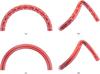 |
Fig. 1 Figures depicting the changing internal topology of a flux tube caused by its large scale writhing. Panel a) depicts a twisted bundle of curves whose axis is a planar curve, while b) depicts the same field after a kinking deformation, showing how a section of the bundle at its apex has straightened out. Panels c) and d) depict corresponding figures but for an initially untwisted bundle. The apex becomes twisted through the kinking in d) where twist was reduced in b). |
There is some reason to think that the interplay between the global sigmoidal geometry of the tube and its internal topology might lead to differing behaviour of internally braided and internally twisted flux ropes, as we now explain. A key aspect of the active region studies such as Fan & Gibson (2007), Kliem et al. (2004, 2010, 2012), Leake et al. (2014), is that cylindrical flux ropes with significant internal twisting become unstable and kink (writhe) in order to relieve the energy associated with twisting, by reducing the amount of twisting through counter-rotation (see Fig. 1). Mathematically one can quantify this exchange through the Călugăreanu theorem (Berger & Prior 2006). This concerns the magnetic helicity H of a flux tube, a topological measure of the flux-weighted inter-winding of its field lines which is an ideal invariant and approximately conserved in the corona (Berger 1984). The Călugăreanu theorem shows how the helicity can be linearly decomposed into total twisting  of the field lines around the tube’s axis and the writhe
  , a measure of the non-planar contortion of the tube’s axis and the extent to which it winds around itself globally, i.e.
 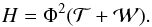 (1)Here Φ is the net magnetic flux across the tube’s cross section.
The most common starting configuration in a number of erupting flux rope studies is a section of a toroidal tube (e.g. Fan & Gibson 2007; Kliem et al. 2004, 2010, 2012; Leake et al. 2014). In this case  and the tube’s helicity is entirely due to twisting. As the tube kinks, tends to increase in magnitude, so to conserve H the twist decreases in magnitude, as shown in Fig. 1a → b. Figures 1c and d demonstrate that the loss of twisting is due to the contortion of the flux rope’s axis, providing a counter-rotation to the twisting. However, for a braided field such as the pigtail braid superimposed on a kinked flux rope structure, the total contribution due to the linking perpendicular to the direction of the tube’s axis (a generalisation of ) is zero. This reflects the well-known property of the pigtail braid that non of its strands are pairwise interlinked (Berger 1991), so that it adds nothing to the sum H. Thus helicity conservation prevents the tube from lowering braiding by deforming with an increase in writhing. Geometrically this represents the fact that contortion of the tube’s axis can only provide a counter-rotation, which cannot undo a more intricate braiding pattern in the same way it can twisted structure. So the path to decreasing energy through writhing used by the kink instability would not likely be available for more complex braided flux ropes. This observation makes it plausible that it might not be energetically beneficial for a braided tube to kink, and thus that flux tubes with braided field patterns may well have more stable global morphology than their twisted counterparts, all else being equal.
In what follows we test the hypothesis that braided internal structure could stabilise flux ropes in situations where twisted fields become unstable, using a number of example fields.
2. Creating the flux ropes
We now briefly review the technique for creating magnetic flux ropes with arbitrary axial geometry introduced in Part I of this study (Prior & Yeates 2016). We consider ropes embedded in a Cartesian coordinate system (x,y,z). The ultimate aim is to define a tube (of possibly varying radius) whose interior is filled with a specified set of curves; that is to say, we specify its precise topology. A divergence-free field B whose field lines have this exact topology is then created.
The tube’s axis is specified by a curve r(s): [ 0,L ] → R3. A right-handed moving orthonormal basis (d1,d2,d3) is defined for r with d3 = r′(s) / | r′(s) | being the unit tangent vector of r, d1 a vector field always normal to d3 (d1·d3 = 0) and d2 = d3 × d1. We shortly give an extra condition to define d1 uniquely. The use of such moving frames is standard in thin rod and polymer elasticity (Antman 2005). This basis can then be extended to form a curvilinear coordinate system by defining a map T(s,ρ,θ): [ 0,L ] × [ 0,1 ] × S1 → R3 as  (2)This coordinate system is shown in Fig. 2a. The radius function R determines the (possibly) varying width of the tube, whilst the coordinate ρ marks concentric tubular surfaces foliating the domain. The evolution of this basis with s, the arclength of r(s), is determined by the linear ODEs
 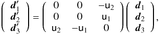 (3)where u1 and u2 are functions determining the curvature of r1 about the two orthogonal directions d1 and d2. Equation (3) defines d1 uniquely up to an initial condition. Readers familiar with the differential geometry of tubes will recognise that, for this choice of basis, d1 is parallel-transported along r (Bishop 1975). The precise means of constructing this basis for a given curve r was detailed in part I of this study (Prior & Yeates 2016). This choice of framing means that the curves of fixed coordinates R = const. and θ = const. will follow the shape of the tube (Fig. 2b), i.e. it is the simplest possibly topology given the tube’s shape. One can then impart more complex topology on the tube by specifying functions ρ(s) and θ(s) for each curve of the field, a simple example being ρ(s) = const. and
  for all curves, which will generate a twisted tube with total twist
  (Fig. 2c).
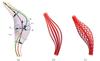 |
Fig. 2 Illustrations of the curvilinear geometry used in this study. Panel a): curvilinear coordinate system T(s,ρ,θ); also shown in green is an example curve as well as the orthonormal basis (d1,d2,d3). Panel b): domain T filled with field lines created by parallel transport, while panel c): domain T filled with twisted field lines. |
2.1. Generating the magnetic field
A set of curves determined by the functions ρ(s) and θ(s) determine a unit tangent field N at all points in the domain T. We turn this field into a divergence-free field B by writing B = φN and solving the PDE  (4)whose solution via the method of characteristics (integrating along field lines f(s)) is
  (5)where φ0 is the distribution of φ on the surface s = 0. In summary, to define the flux rope magnetic field we have to specify:
-
1.
The tube’s basic geometry through r(s) and the radius function R(s), which determines its (possibly) varying thickness.
-
2.
The internal topology, through functions ρ(s) and θ(s) determining the paths of curves in the domain.
-
3.
The magnetic flux distribution φ0 on one end of the tube.
We then integrate (5) to determine the full field. A further embellishment of this process is to select a finite number of curves ri from the original tube T and to create smaller tubular fields surrounding each curve ri. In this way, a pigtail braided field with sigmoidal axis was created in Part I (an example is shown later in Fig. 5). A second approach to increasing the complexity of the field is to define fields which partly overlap, creating a composite field with more complex internal topology. This is used in what follows to develop a version of the braided field used in Yeates et al. (2010, 2015), Wilmot-Smith et al. (2011).
There are a number of technical issues involved in creating such fields in practice, particularly with regards to the matter of sampling the field on a finite grid for numerical simulations and ensuring it is sufficiently divergence free when discretised. We refer the reader to Part I for details, it suffices here to say these issues were surmounted and we have reliable code which creates the fields. One other issue dealt with in the original study is the question of how well the tubular co-ordinate system is defined, which depends on the geometry of the curve r(s). In Part I, specific conditions for the positive-definiteness of the Jacobian of the map T were established. The fairly obvious conclusion was that curves with very high curvature can only support tubes with a restricted width, in order for this coordinate system to make sense. For the typical flux ropes seen in the coronal region this is not generally an issue.
2.2. Embedding the rope over a inversion line
In Part I, we demonstrated how to embed the flux rope over the inversion line of a specified boundary flux distribution, where filaments are generally observed to form (Mackay et al. 2010). The basic idea is obtain a smooth 2D curve σ(s) fitted to the inversion line and then choose so height function z(s) to create a curve r(s) = (σx(s),σy(s),z(s)) which would then project down onto the inversion line (some examples are shown in Fig. 3). This curve can then be used as the axis of the tube T containing the flux rope.
3. Magnetic fields used in this study
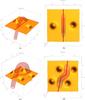 |
Fig. 3 Boundary flux distributions for the background field in this study, and their associated tubular domains T. Panels a) and b): dipolar flux distribution, with the straight inversion line shown in red. Panels c) and d): sigmoidal dipole distribution, with Z-shaped inversion line. |
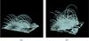 |
Fig. 4 Magnetic field lines of the background fields used in this study: a) dipolar, and b) sigmoidal dipole. |
3.1. Background field
We embed our tubular field Bt in a force-free background Bb, ∇ × Bb = αBb, which is an appropriate choice for the low corona where the magnetic pressure dominates the plasma pressure (e.g. Priest 2003). The tubes are defined in a domain {− π ≤ x,y ≤ π,0 ≤ z ≤ 3π}. For simplicity here we choose a linear force-free field on the volume z> 0, specified by choosing a constant α and a photospheric (z = 0) flux distribution.
The first field, generated from a dipolar distribution, is similar to that used in Török & Kliem (2005), Mackay & Van Ballegooijen (2006), MacTaggart & Hood (2009b), Kliem et al. (2010), Aulanier et al. (2010), Cheng et al. (2011), Kliem et al. (2012), Hood et al. (2012), Archontis et al. (2014). The second, a field generated from a staggered pair of dipoles, is the type used in Prior & Berger (2012) and in Part I. The inversion line of the boundary flux has a noticeably sigmoidal morphology and is dominated by a deformed-arch topology. In what follows we refer to this field as the “sigmoidal dipole”. The dipolar field is chosen because the behaviour of a twisted flux rope embedded in this field is well documented; in particular, we know it should lead to instability and large scale rotation, if the flux rope twist exceeds a critical value (Török & Kliem 2005). The aim will be to see how braided fields relax in a similar situation. The sigmoidal dipole distribution is then used to see if the conclusions drawn from the dipolar case can be generalised. We only actually present results for α = 0 for the dipolar case and α = 0.5 for the sigmoidal dipole field (this is the value used in Part I). Though simulations with differing α values were run, the differences in evolution proved not to be significant.
For the dipolar case we choose the boundary flux to take the form 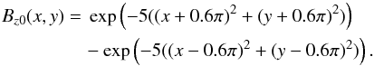 (6)This distribution and its inversion line are shown in Figs. 3a and b, along with the flux rope domain T in which we embed our fields. Note that the flux rope itself will generate two additional sources to the boundary flux distribution. The sigmoidal dipole background is given by
 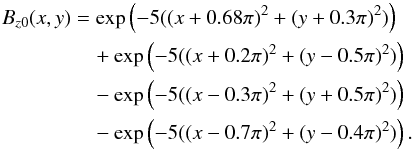 (7)The distribution and its inversion line are shown in Figs. 3c and d, along with the flux rope domain T in which we embed our fields. The inversion line has has a z-shaped morphology meaning when we insert our flux rope it will have a sigmoidal morphology at the start of the simulation. In both cases we then generate the linear force-free field in z> 0 using the method detailed in Prior & Berger (2012). Example field lines for both cases can be seen in Fig. 4: in both cases there is a clear arcade of field lines looping over the inversion line.
3.2. Internal rope topologies
In this paper, we consider four different internal structures for the flux rope, each embedded in the same tube T (as shown in Fig. 3).
3.2.1. Uniform twist
As mentioned above, the choices R = const. and define a field with uniform twist and a total rotation of  radians. In the flux rope simulations of Török & Kliem (2005), a (part) toroidal tube embedded in a dipolar potential, a value of
  was found to be the threshold twist above which the tube was kink unstable. In both cases we chose values above this threshold leading the ropes to kink. The tube R is 0.5.
3.2.2. Pigtail braid
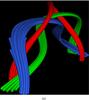 |
Fig. 5 Field lines of the pigtail field used in this study. |
The pigtail braid, shown in Fig. 5 is made up of three flux ropes ri which interlink within a tube T, whose axis r has the morphology of the inversion line. The axes of the three sub-tubes are defined by the functions 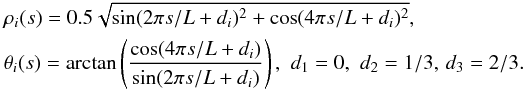 (8)We then create tubular fields Bi in tubes Ti of fixed radius Ri = 0.2 around each of these axes (Fig. 5). In this study we choose the fields to have no internal twisting.
3.2.3. B4 braid
This is based on the numerical experiments of Wilmot-Smith et al. (2009, 2011), Russell et al. (2015), where a family of braided magnetic fields were created using series of n opposing pairs of rotations through an angle π rad at staggered distances along the tube’s length. In this case we use 4 pairs of opposing twist so this would be a B4 field (in the notation of Wilmot-Smith et al. (2009) this would be an E4 field, but we prefer “B” to indicate “braided”). In this study we once again define a curve r which follows the inversion line of the tube. We then define two curves ri,i = 1,2 as 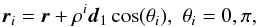 (9)with d1 the parallel-transported vector field, defined by the solution to (3). These curves are then used to define two tubes Ti,i ∈ 1,2. The values of ρi and the tube radii Ri are chosen so that the tubes have significant overlap (Figs. 6a and b). For the dipolar case we choose Ri = 0.4 and ρi = 0.3, and for the sigmoidal dipole case Ri = 0.5 and ρi = 0.35. We then define the fields within the tubes with the following topology functions:
 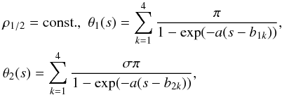 (10)with σ = −1 and b11<b21<b12<b22<b13<b23<b14<b24. This creates a series of staggered half twists of the field, with the twist occurring sequentially in tube T1 then T2 then T1 again etc. The choice σ = −1 means that the rotations have opposing chirality. In practice the values of b1i,b2i and a are chosen so that there is no overlap (when one tube has twisted field lines, the field lines of tube 2 are created by parallel transport). It can be seen in Fig. 6c that a subset of the curves are then braided. These two prescriptions of θ1 / 2 can be used to make fields B1 and B2; the B4 field is their sum BB4 = B1 + B2. If the tube axis is a straight line (the tube a cylinder), then the helicity of BB4 is zero (Wilmot-Smith et al. 2009). In our more general tube geometries there may be a non zero helicity due to the writhe of the tube axis (see Berger & Prior 2006; Prior & Yeates 2014).
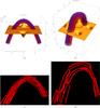 |
Fig. 6 Visualisations of the B4 and T4 fields. Panels a) and b): overlapping tubular domains in the dipolar and sigmoidal dipole backgrounds respectively. Panels c) and d): magnetic field lines of the corresponding field. In B4 c) the sequentially applied twists have opposing chirality and field lines are braided, whilst in T4 d) the twists have the same chirality and field lines are twisted (non-uniformly). |
In Wilmot-Smith et al. (2011) a similar field, embedded in a cylindrical tube, was shown to split into two force-free flux ropes of opposing twist through reconnection, entirely contrary to the Taylor relaxation hypothesis. An explanation for this phenomenon was proposed recently by Russell et al. (2015) though it is beyond the scope of the discussion here.
3.2.4. T4 field
The T4 field is the same as the B4 field given by Eq. (10) but with σ = 1, so that the sequential twists applied to each tube have the same sign. Even when the axis curve r is straight this field has a net helicity as it has a net sense of rotation (Fig. 6d). As the notation T4 indicates, this is a twisted field, though the twisting is non-uniform. In Wilmot-Smith et al. (2011) a similar field embedded in a cylindrical tube was shown to merge into a single force-free flux rope.
3.3. Boundary flux
For each field we must specify a boundary flux distribution φ0(ρ,θ) at one end of the tube. As in Part I, we choose a radially-symmetric distribution φ0(ρ,θ) = 0.5φc(cos(πρ)−1), with φc a constant determining the maximum strength of the field. In our simulations the maximum strength of the background field is 1, so choosing the value φc dictates the field strength of the tubular field relative to the background. We ran simulations with values of 1, 3 and 6. The larger the relative strength of the flux tube, the less its motion was constrained by the background field, but in general there were no significant differences in the evolution of the fields that merited presenting the results for each choice of φc. In what follows we present (primarily) the results for φc = 3.
4. Numerical simulations
The superpositions Bt + Bb for each of the fields described in Sect. 3 define a set of initial configurations for our magnetic field. These fields will not generally be in equilibrium, unlike the toroidal twisted fields used in Fan & Gibson (2007), Kliem et al. (2004, 2010, 2012), Leake et al. (2014), for which an equilibrium within the background dipole field can be found (Titov & Démoulin 1999; Titov et al. 2014). The relative complexity of the combinations of our background field, tube morphology, and internal structure make finding an analytical equilibrium unfeasible. There is evidence that braiding is a dynamic phenomenon (van Ballegooijen et al. 2014), and it is reasonable that we might see complex internal structures built up relatively quickly in the corona. In this paper, we investigate whether these configurations would either relax to a configuration whose global morphology is similar to the original configuration, or if they undergo significant large-scale motions (like the kink instability). Our prediction is that braided flux ropes (the pigtail and B4 fields) will experience significantly less change in axis geometry (global morphology) than their twisted counter parts (the uniform twist and T4 fields), though both might experience significant changes in internal structure. To keep things simple, we avoid boundary motions. This allows us to focus on the questions of how the processes of ideal evolution and resistive reconnection alter the field.
4.1. Magnetohydrodynamic (MHD) equations
We evolve the initial field Bt + Bb using the Lare3D Lagrangian-remap code (Arber et al. 2001) to solve the resistive-MHD equations on a Cartesian box {− π ≤ x,y ≤ π,0 ≤ z ≤ 3π}, at resolution 264 × 264 × 396. The initial tube’s maximum height is less than 4 so this gives room for any reasonable vertical expansion, which we expect from kink (and or torus) unstable flux ropes in at least one case. On the z = 0 boundary we use line-tied boundary conditions, while on all other boundaries we use Lare’s open boundary conditions, based on a simplified Riemann characteristic model. This allows waves to exit the system, a feature not present in the simulations of Part I which used line-tied conditions on all boundaries. The code solves the following equations: 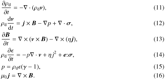 Here ρd is the mass density, v the plasma velocity, B the magnetic field, j the current density, p the plasma pressure, σ the stress tensor, ϵ the specific internal energy, η the resistivity, e the strain tensor, and γ = 5 / 3. The equations are non-dimensionalised in Lare by setting a length scale L0, magnetic field strength B0 and density ρ0; we chose L0 = B0 = ρ0 = 1. In these units, one unit of time is equal to the time taken by an Alfvén wave with B = ρ = 1 to move a unit distance in the box. The viscous term ∇·σ in Eq. (12) has a shock viscosity to prevent unphysical oscillations and approximate the jump in entropy across shocks. In addition we used a background viscosity of 0.01 as an aid to numerical stability. Whilst in practice we would expect little viscosity in the corona, this value was used to reduce the computational time so that significant evolution of the fields could be observed. This approach is consistent with other studies (e.g. Fan & Gibson 2007; Kliem et al. 2004, 2010, 2012; MacTaggart & Hood 2009b; Hood et al. 2012). The shock viscosity takes the form given in Bareford et al. (2013), and we use the same successful parameter values ν1 = 0.1, ν2 = 0.5. There is a corresponding heating term e:σ in Eq. (14). The simulations presented here use a uniform resistivity of 5 × 10⁻⁴ (a value found by experience to be similar to the numerical resistivity for the grid we employ). The initial velocity is assumed to vanish everywhere so that any motion will result from the field attempting to relax to equilibrium. Finally we initialise with ϵ = 0.01 and
  , i.e. a mass density that decays with the background field. In Part I, constant values of ρd = 1 and ϵ = 0.01 were used; the only other difference in the system and its parameters from those used in Part I is the addition of a non-zero background viscosity as discussed above. We adopt the varying density here as it was shown in Török & Kliem (2003) to produce a much more significant flux rope eruption than a constant initial distribution. Since the aim is to compare the difference in behaviour of the rope’s global morphology we would like to promote such changes as much as possible. Finally with the non-dimensionalisation used in Lare the plasma beta can be shown to be 2ρϵ(γ − 1) /B2, which for our choice of density is
 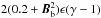 (Arber et al. 2001). In regions originally occupied by only the background field (strength 1 at the z = 0 boundary) this is ≈ 0.016. The typical strength of the initial rope field is 3 and we have placed it in a region where the background field is weak to negligible (the inversion line). so the plasma beta is approximately 0.014. Both values are reasonable for the corona (Priest 2003).
The simulations were run until the time step (imposed by the CFL condition) became impracticably small. This was likely the result of a build up of significant small scale flows through reconnection, as well as the possibility of boundary effects (it is hard to avoid some degree of wave reflection in such simulations; see the discussion in Hood et al. 2012). As we shall see, there was a significant drop in the Lorentz force for each simulation and the magnetic energies were found to approach asymptoptic limits.
4.2. Diagnostics
We follow the same approach to analyse the changing flux tube geometry as adopted in Part I. Firstly we plot magnetic field lines anchored at the initial base of the tubular field Bt at t = 0, the points on z = 0 at which Bz> 0. In what follows we refer to the field lines emanating from this subdomain as the “core” field. The likely occurrence of reconnection with the background field means some of these field lines may not end up being part of the rope, and other field lines not initially forming part of the rope may reconnect to join the rope’s bulk. That said, we feel this is a sensible means of gauging the changing geometry of the rope, an assumption justified by the plots detailed in what follows. In panels a−c of Figs. 7, 9, 10, 12 and 15 these curves are shown embedded in the background field to display their effect on this field. The three strands of the pigtail field are given different colours in an attempt to observe the reconnection-led mixing of the strands. In addition, we plot the core field as seen in projection from above (panels d−f of Figs. 7, 9, 10, 12 and 15). This is done in order to observe the rotation (or lack thereof) of the core. We also plot contours of a fixed current density in order to observe the changing current structure of the fields (panels g−i Figs. 7, 9, 10, 12 and 15). A value | j | = 1 was chosen as it was found to have significant representative structure across the timescale of all simulations.
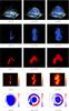 |
Fig. 7 Figures depicting the evolution of the uniform twist field embedded in a dipolar background field. The three times used are t = 0,4.75,9.5 shown from left to right respectively. Panels a)−c): core embedded in the background field. Panels d)−f): core from above. Panels g)−i): current contours of the field. Panels j)−l): emission proxy E(x,y). Panels m)−o): local twisting distribution Lf(x,y). |
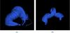 |
Fig. 8 Visualisations of the internal structure which develops in the uniform twist field, showing a) the core field at t = 9.5; and b) a subset of radius 0.1 whose structure is significantly more kinked than the morphology visible in a). |
4.2.1. Emission proxy E
Given a point P in the domain, we trace the field line passing through it. We then integrate the square of the current density along this field line and average. We label this quantity  ; the emission proxy is then an attempt to imitate the line-of-sight viewpoint by integrating in z
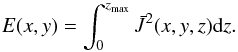 (17)This is not intended to be a direct prediction of how the rope would be observed at a particular wavelength in coronal observations, as that would require inclusion of more detailed thermodynamics in the model (e.g. thermal conduction). It is rather a first order approximation accounting for only ohmic heating and assuming that heat conduction is much faster along magnetic field lines than across them. This proxy has been used in previous studies of non-linear coronal field models where accurate density and temperature distributions are not available (e.g. Cheung & DeRosa 2012). We calculate this quantity across the whole plane z = 0 (panels j−l of Figs. 7, 9, 10, 12 and 15).
4.2.2. Local twist distribution Lf
A quantitative measure of the field’s internal geometry which we measure is the average local twisting of each field line. For a field line f(l) of arclength L whose footpoint coordinates are (xf,yf), we define the integrated quantity 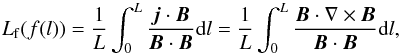 (18)which represents the mean rotation of the local field lines around f(l). It is not quite the same as the twist which appears in the Călugăreanu theorem, but it is a reasonable measure of the effective twisting of local field lines (Liu et al. 2016). For a linear force-free field, j·B = αB·B and Lf is just the linear force-free parameter α, which would be constant throughout the domain. This quantity was calculated for relaxing braided and twisted cylindrical fields in Wilmot-Smith et al. (2011), Yeates et al. (2015). These authors found that a twisted field relaxed to a force-free state with a single sign of α within the tube, although the surrounding background field prevented it from reaching the spatially constant α predicted by the Taylor relaxation hypothesis. By contrast, they found braided tubes to relax to form two force-free flux tubes with equal α values but opposite sign, entirely contrary to the Taylor hypothesis. Similar findings were observed in Part I. Here we consider the distribution Lf(x,y) of average local twisting for each field line anchored at points (x,y) (panels m−o of Figs. 7, 9, 10, 12 and 15 ). Since we are really interested in the flux rope core we restrict this measure to the (x,y) coordinates of the fields core (this is a disjoint domain for the pigtail field).
5. Results: dipolar background
5.1. Uniform twist
As is clear in the field line plots Figs. 7a−f, the field has undergone the expected kink instability with a significant S-shaped morphology developing. The current contours, Figs. 7g−i, and emission proxy E(x,y), Figs. 7j−l, reflect this kinking. Previous simulations (Fan & Gibson 2007; Kliem et al. 2004, 2010, 2012) indicate that the evolution would have to be followed for a significant time in order to observe whether the rope erupts or not. However, in this study we would like to compare a number of different fields, and we judged the significant extra computational time to be unnecessary given that the eventual evolution has been studied in significant detail previously.
The local twist distribution Lf(x,y), Figs. 7m−o, is initially dominated by a significant domain of constant negative value, consistent with the uniform twist specified in the initial field. By t = 4.9 this core has shrunken significantly. At t = 9.5 the core is relatively small; it is also surrounded by a thin positive ring and then a second negative ring. This indicates that a rope has developed in the centre of the core which has a different morphology from the outer structure seen in Figs. 7a−f. This is confirmed in Fig. 8 where the core field is plotted, first with a radius 0.5 at t = 9.5, the radius of the initial core (panel a), and second with a radius of 0.1 at the same time (panel b). The morphology of the inner core b is significantly more kinked than the outer core a, though the chirality of this kinking is the same for both fields (both are S-shaped).
5.2. Pigtail braid
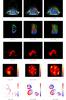 |
Fig. 9 Figures depicting the evolution of the pigtail field embedded in a dipolar background field. The three times used are t = 0,4.75,9.5 shown from left to right respectively. Panels a)−c): core embedded in the background field. Panels d)−f): core from above. Panels g)−i): current contours of the field. Panels j)−l): emission proxy E(x,y). Panels m)−o): local twisting distribution Lf(x,y). |
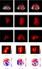 |
Fig. 10 Figures depicting the evolution of the B4 field embedded in a dipolar background field. The three times used are t = 0,2.25,4.5 shown from left to right respectively. Panels a)−c): core embedded in the background field. Panels d)−f): core from above. Panels g)−i): current contours of the field. Panels j)−l): emission proxy E(x,y). Panels m)−o): local twisting distribution Lf(x,y). |
The field line evolution of the pigtail field, represented in Figs. 9a−f, is somewhat difficult to interpret. The initial configuration (a and d) is significantly affected by the background field (through the sum Bt + Bb), as evidenced by a number of field lines which peel off the initial braided structure. (The pigtail nature of the initial field is clearer in the current contour plot of Fig. 9g.) By contrast to the twisted field (Fig. 7), there is no obvious global rotation of the structure, but it does expand significantly. It appears that there are still collections of field lines of the same colour in panels b and c of Figs. 9, indicating some of the braided structure is preserved. Aside from this observation it is hard to draw any clear conclusions regarding the geometry of this field’s evolution from these figures.
The current contours shown in Figs. 9g−i show that the braided structure evolves into a significantly fractured structure, with a single large twisted sheet between the core and the background arcade. By comparison the twisted flux rope maintains its tubular structure and has an untwisted current sheet covering the internal structure (Figs. 7g−i). One can view this sheet as the edge of the core field, while the more complex sheet structure for the pigtail case reflects how this field maintains some separation of the original three strands present in Fig. 9a. This is consistent with the observation that the fields lines of differing colours still show significant organisation (panels b and c of Figs. 9).
The emission proxy E(x,y) initially indicates the braided structure, as well as having a significant contribution from the field lines peeling off the braid (Fig. 9j). By t = 4.5, Fig. 9k, the emission has dispersed significantly though there remains some trace of the initial pigtail structure over the inversion line. In l, t = 9.5, we see regions of relatively high E values either side of the inversion line (top left and bottom right), representing field lines that have reconnected with the background field. There is also still a faint trace of the initial pigtail structure.
The t = 0 local twisting distribution Lf(x,y) is mostly zero inside the braid footpoints (Fig. 9m), as the field lines inside the sub-tubes have no twist. There are some thinner domains of positive and negative twisting on the boundary, which result from the influence of the background field in the sum Bb + Bt. At t = 4.75 (Fig. 9n) and t = 9.5 (Fig. 9o), the field has significant internal twisting structure. There are regions for which Lf has both positive and negative signs, and there is a good degree of mixing of these regions. It is hard to draw any simple conclusions other than the fact that the internal topology of the field is still significantly complex and far from the uniform Lf value one would expect for a linear force-free flux rope (the core has not reached the Taylor state).
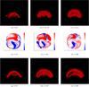 |
Fig. 11 Figures depicting the tendency of the B4 field to split into two flux ropes of opposing sign. Panels a)−c) the core field shown in Figs. 10a−f as viewed from the side. Panels d)−f) local twisting distributions Lf(x,y) of the B4 field for a simulation, whose core field lines are shown in panels g)−i), and whose maximum field strength is comparable to that of the background field (the flux rope of the field in panels a)−c) is a factor 3 stronger than in panels g)−i)). |
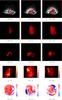 |
Fig. 12 Figures depicting the evolution of the T4 field embedded in a dipolar background field. The three times used are t = 0,2,3.9 shown from left to right respectively. Panels a)−c): core embedded in the background field. Panels d)−f): core from above. Panels g)−i): current contours of the field. Panels j)−l): emission proxy E(x,y). Panels m)−o) the local twisting distribution Lf(x,y). |
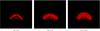 |
Fig. 13 Figures depicting the tendency of the T4 field to form a uniformly twisted flux rope. |
5.3. B4 braid
The field line evolution of the B4 field is represented in snapshots at t = 0,2.25,4.5 in Figs. 10a−f. There appears to be little change in global morphology of the field’s core (rotation), although we shall see shortly that there is a significant change in the internal structure. It is also clear that there is a significant degree of reconnection with the background field. The current contours evolve to develop multiple smaller current structures in the core’s interior (Fig. 10g−i), in addition to a larger sheet structure which encases the core field. The formation of small scale structures is consistent with the B4 cylindrical braiding experiments of Wilmot-Smith et al. (2011), though the larger encasing current sheet is unique to this simulation, resulting from the background field.
The emission proxy E(x,y) is shown in Fig. 10j−l at t = 0,2.25,4.5. The pattern remains consistent, save a drop in peak value. There is a clear contribution from the core’s axis at the centre of the distribution – this is directly above the inversion line of the photospheric flux distribution. In addition, there are contributions on either side of the main axis from field lines that connect between the background field and the B4 field, visible in Figs. 10a−f. The distribution is similar to that of the pigtail field (Figs. 9j−l), except the emission above the inversion line is much more significant for the B4 field (relative), consistent with the relative lack of expansion shown by this field by comparison to the pigtail field.
The local twisting distribution Lf(x,y) (Figs. 10m−o) initially has two islands of strong positive and negative values, in addition there is a good deal of mixing of thin contorted strips of positive and negative value. This is reasonably consistent with the similar distribution of the field used in Wilmot-Smith et al. (2011) – cf. Fig. 10m with Fig. 11 of Wilmot-Smith et al. (2011), where Lf is labelled α∗. The mixing is slightly less extreme our case, which is probably due to the spacing of the twists in the field. Nonetheless there is still significant mixing indicating a complex internal topology. The evolution seems to lead to a decrease in area of the initial positive and negative islands (Figs. 10n and o).
In Fig. 11a−c, we see the fields of Figs. 10d−e viewed side on. It is clear the field splits into two distinct flux ropes of opposite chirality (as in Wilmot-Smith et al. 2011), however, it is clear that there are still multiple field lines which cannot be assigned to either tube. This explains the mixed patterns still surrounding the flux rope twisting islands seen in Figs. 10n and o. On this subject, we briefly report on the simulation of the B4 field with a lower value of the peak flux φc = 1, so that the background field strength is similar to the strength of the B4 field. In this case the simulation ran for longer, allowing further reconnection to reduce the mixing of the Lf(x,y) distribution significantly (Fig. 11d−e). This corresponds with a much cleaner separation of the field into two flux ropes (Fig. 11f−h).
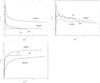 |
Fig. 14 Scaled energy plots for the four field types embedded in a dipolar background with energies scaled by their initial values. Panel a): difference in (scaled) magnetic energy Eb from the initial value; b): scaled kinetic energy Eke, and c): difference in scaled internal energy Eint from its initial value. |
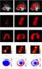 |
Fig. 15 Figures depicting the evolution of the uniform twist field embedded in a sigmoidal dipole background field. The three times used are t = 0,7.5,15 shown from left to right respectively. Panels a)−c): core embedded in the background field. Panels d)−f): core from above. Panels g)−i): current contours of the field. Panels j)−l): emission proxy E(x,y). Panels m)−o): local twisting distribution Lf(x,y). |
5.4. T4 field
The field line evolution of the T4 field is represented at t = 0,2,3.9 in Figs. 12a−f. There is little obvious change in global morphology of the field’s core, similar to the B4 field lines (Figs. 10a−f), though there is a little more expansion of the core for the T4 field. At t = 2 a significant current sheet has formed at the bottom of the core field (Fig. 12h), but unlike the B4 field (Fig. 10g−i) there is no small scale structure. By t = 3.9 (Fig. 12h) this sheet has increased in area.
The evolution of the emission proxy E(x,y) is shown in Fig. 12j−l. It differs significantly from the B4 fields evolution (Fig. 10j−l). At t = 0 (Fig. 12j) there is a clear contribution from the core’s central axis directly above the inversion line of the photospheric flux distribution, with additional contributions on either side of the main axis resulting from the field lines which peel off the structure due to interference of the background field and the T4 field (see Figs. 12a−f). By t = 2 (Fig. 12k) the central core distribution appears to have formed a thin S-shaped morphology (which is relatively weak by comparison to the reconnected field lines). By t = 3.9 (Fig. 12l) the central core’s contribution has receded to a thin S-shape, the strongest contributions are from the reconnected field lines.
The local twisting distribution Lf(x,y) is initially dominated by a large island of positive twisting (Fig. 12), this is to be expected as the initial twists of the T4 field are all right-handed. This distribution is qualitatively similar to the initial Lf(x,y) distribution of the uniform-twist field shown in Fig. 7m−o (swapping blue for red as the earlier field has negative twist). As the field evolves, the initial island shrinks in relative size indicative of significant reconnection with the backgound field. The smaller island forms a more uniformly twisted core, as confirmed in Fig. 13a−c where we see the field from the side. This is consistent with the simulations of Wilmot-Smith et al. (2009), Yeates et al. (2010).
5.5. Comparative conclusions
Comparison of the uniform-twist and pigtail fields suggests that increased complexity of the rope’s internal structure restricts the potential for significant global changes in morphology, save expansion of the tube. This is further reinforced by the fact that the B4 field shows no significant large scale change in morphology, rather a significant change in internal topology through splitting. It is also true that the T4 field does not rotate, despite forming a flux rope, though it is likely the twist is not sufficient for the kink instability to occur.
With regard to evolution of the internal structure, the two “twisted” fields – the uniform-twist and T4 fields – both have local twisting distributions Lf(x,y) with a dominant sign, indicative of the initial twisting in the fields (negative for the uniformly-twist field and positive for the T4 field). By contrast, the pigtail and B4 fields seem to relax to maintain a (rough) balance of both positive and negative twist. So the initially braided fields maintain an internal topology which is topologically distinct from a single twisted flux rope.
In comparing the two braided fields – the pigtail and B4 fields – we note that the initially complex B4 field develops a significant degree of organisation through the formation of two distinct flux ropes. This corresponds to a significant decrease in the mixing of positive and negative twisting in its Lf(x,y) distribution (Fig. 11g−i). By comparison the pigtail Lf(x,y) distribution quickly develops a significantly mixed distribution, indicative of a complex internal topology, and this does not seem to have simplified by the end of the simulation. This is likely due to the B4 field being a single, well-mixed, tubular field whose internal topology is changed by internal reconnection, whilst significantly altering the topology of the braided field would require significant reconnection of three distinct fields.
These differences in internal structure might well translate into observable differences; indeed, the emission proxy distributions E(x,y) for each case differ significantly. The uniform-twist field starts with a clear emission line which deforms to form a very obvious sigmoidal pattern. The pigtail braid on the other hand evolves into a significantly fractured emission pattern. Partly this may be because of the interaction of the background field and the core, which seems to be more significant than in the uniform-twist case. It is also a result of the fact that the braid cores are able to expand without significantly altering the field’s topology (thus reducing the current). The more complex internal entanglement of the T4 and B4 fields seems to dramatically inhibit expansion and rotation by comparison. This is reflected in emission patterns which change much less significantly over time. The B4 field – the most complex internal topology – leaves a significant trace above the inversion line, much like the twisted field initially, but this line does not change (save changing emission magnitude), consistent with the assumption that braiding/complex entanglement can inhibit large scale motion. We also note that the more complex internal topologies – pigtail, B4 and T4 – tend to interfere with the background field more than the uniformly twisted field, evidenced by the number of field lines which peel off the core field structure in panels a−f of Figs. 9, 10, and 12 and their significant contribution to the emission proxy (panels j−l of Figs. 9, 10, and 12).
The evolution of the magnetic energy Eb, kinetic energy Eke and internal energy Eint, for the four fields, is shown in Fig. 14. The initial magnetic energies of the four fields are: uniform−twist = 2.18, pigtail braid = 1.861, B4 braid = 3.33914, and T4 Field = 3.33901. In Fig. 14 we rescale all energies by their initial magnetic energy Eb(0) for relative comparison. We also scale the time by an Alfvén time  , using the root of the magnetic energy as a proxy of the mean strength of each field. The scaled differences Eb(t) − Eb(0) are shown in Fig. 14. In all cases the magnetic energy is decreasing exponentially, with a rapid loss in energy associated with the field’s initial expansion. The pigtail, B4, and T4 energies drop by the largest amount, and the B4 and T4 fields show a sharper initial fall than the pigtail field. The pigtail, T4 and B4 differences appear to be plateauing, whilst the uniform-twist field still has significant gradient at the last point of observation. This is because the uniform-twist field is still in the process of rising when the simulation was stopped. The fact that the B4, T4, and pigtail fields lose a larger percentage of their initial energy suggests that the fields are indeed showing a preference for energy reduction through internal topological changes rather than large scale morphological changes.
The kinetic energy shows a sharp rise in all cases, due to the rapid expansion of the tubes, then begins to drop steadily. The decrease for the B4 and T4 fields is significantly faster. Indeed for the field shown in Figs. 11d−f, for whom the relative strength of the field is comparable to the background, the kinetic energy drops close to 0. The twisted field is still rising so we should expect its kinetic energy to remain non-zero. None of the pigtail simulations had vanishing kinetic energy. Further analysis of these showed that the significant velocities are between the three pigtail strands, suggesting the continued presence of significant reconnective activity.
The internal energy of the B4, T4, and pigtail fields shows a rapid initial increase falling to a less rapid but steady increase. The twisted field does not show such a rapid initial increase. Further analysis showed internal energy to be dominated by viscous dissipation. It is likely the slower initial increase of the twisted field is caused by its kinking rather than solely expanding.
As a final note, we observe that the energy plots for the B4 and T4 fields are remarkably similar, though not identical. Several factors likely explain this. Firstly, the initial energies of the two fields are the same and both have the same total magnitude of twist. Secondly, the bulk change in shape of the two tubes, namely expansion but no rotation, is very similar. So changes in the background field would be quite similar (cf. Figs. 10a−c and 12a−c). We conclude that the energy is dominated by these large scale considerations, i.e., energy totals and bulk changes in structure. The differences due to local reconnection inside the tube seem to affect the energy to a lesser degree.
Finally the Lorentz force of all fields shows a significant decrease. For the uniform twist field, at t = 0 the maximum value of J·B/B2 is 42.8251 and the mean value is 0.061. At t = 9.5 the maximum value is 0.912 and the mean value 0.016. For the pigtail field the t = 0 maximum value is 38.2371 and the mean value 0.16722, at t = 9.5 the maximum value is 1.694 and the mean value 0.0161. For the B4 braid the initial maximum value is 56.2325 and the mean value 0.162003 at t = 4.5 the maximum is 3.2096 and the mean value 0.02428. For the T4 field the initial maximum value is 56.6086 and the mean value 0.161798 at t = 3.9 the maximum is 2.17032 and the mean value 0.021223. In all cases this reflects significant relaxation towards a force-free state.
6. Results: sigmoidal dipole background
Simulations with all four internal topologies were also run with tubes embedded in the sigmoidal dipole background. In general the results confirmed the observations of the dipolar case. In order to keep this report concise we do not detail the results here, except for the twisted field, which was the one case in which a genuinely novel observation was made.
6.1. Uniform twist
The field line evolution is depicted at t = 0,7.5 ,15 in Figs. 15a−f. Panels a−c indicate expansion of the core and, in addition, a comparison of c to a and b indicates that the apex of the field is rising, similar to the dipole case (Fig. 7), though perhaps less markedly. This expansion is also evident in the current contour plots of Figs. 15g−i. By contrast to the dipolar case, the rotation of the field is not of a consistent chirality. The change in morphology evident in Fig. 15d to e, suggests a counter-clockwise rotation of the apex of the core; whilst the change in morphology observable in Fig. 15e to f indicates a clockwise rotation. This observation is confirmed by the emission proxy E(x,y) shown in Figs. 15j−l. As indicated in Figs. 7d−f the expected apex rotation of a flux rope with negative internal twisting is a counter-clockwise rotation, unless the rope dips, see (e.g. Török et al. 2010). This convention assumes an initially toroidal flux rope so we should not necessarily have expected it to apply in this initially sigmoidal case. But it is of interest that the first attempt to rotate which the core makes follows this pattern. We speculate that this initial rotation is frustrated by the configuration of the background field, which provides a repulsive force resisting the initial kinking motion and the pathway for the field to relax.
The evolution of the local twist distribution Lf(x,y) (Figs. 15m−o) is very similar to the evolution of the dipole case (Figs. 7m−o). There is initially a large island of negative Lf representing the initial uniformly twisted core of the rope. From m to n the magnitude and size of this domain decreases as the rope undergoes expansion and writhing deformations. In n there is a ring of positive Lf values encircling the twisted sub-core. From Figs. 15n to o the only significant change is that a significant section of the positive ring changes from positive Lf to negative Lf. This is likely due to reconnection with the background field.
The main conclusion is that the configuration of the background can have a significant effect on the evolution of the flux rope. There is evidence here that the non-linear evolution of the field resulting from the kink instability is eventually suppressed by the background field.
7. Conclusions
Using a new technique for generating magnetic flux ropes of arbitrary axial geometry and and internal structure, developed in Part I of this study (Prior & Yeates 2016), we created a set of flux ropes embedded in force-free background fields generated from both dipolar and sigmoidal dipole photospheric flux distributions. The flux ropes included a uniformly-twisted field, a pigtail braid field composed of three distinct flux tubes, a single-tube field whose internal field lines were braided (B4), and a similar field T4 whose internal field lines were (non-uniformly) twisted. The last two fields emulate the numerical experiments of Wilmot-Smith et al. (2009), Yeates et al. (2015), Russell et al. (2015) in a field with realistic coronal tube morphology.
Section 5 reported the results of simulations of flux tubes with toroidal axial morphology, embedded in a dipolar background field, with each of the four internal structures. In all cases, they relaxed to states with significantly reduced Lorentz force. The uniform twist field underwent the expected kink instability leading to significant global rotation of the structure; this was reflected in the emission proxy plots which showed a clear sigmoidal morphology. The pigtail field did not lead to any large scale motion, only a significant expansion reflected in the emission proxy plots, which showed dispersion due to expansion of the pigtail’s core (yielding a significantly fractured emission pattern). These conclusions are broadly in line with the preliminary results of Part I. Both the B4 and T4 fields – which had more complex internal field structure – showed significantly less expansion than either the uniform twist or pigtail fields. Comparing the evolution of the B4 and T4 fields, there was noticeably less expansion of the B4 field, a fact particularly reflected in the emission proxy distributions. Both began with a strong line of emission along the initial axis of the flux rope. This structure persisted in the B4 field but was reduced to a weak thin sigmoidal shape in the T4 field. The local twisting distributions Lf(x,y) in the core of the twisted fields (uniform twist and T4) tended to have one dominant sign, whilst the braided fields (pigtail and B4) developed mixed local twisting distributions with roughly equal amounts of both positive and negative twisting. This indicates that the significant difference in initial internal topology between the twisted and braided fields was maintained throughout the simulations.
A second observation was that the B4 and T4 fields both showed the development of significant internal organisation. The B4 field coalesced to form two flux ropes of opposing sign (Figs. 11), whilst the T4 formed one flux rope of roughly uniform twist (Fig. 13). Similar evolution was observed for the numerical experiments of Wilmot-Smith et al. (2009), Yeates et al. (2015), Russell et al. (2015) in which the fields were defined in cylindrical tubes. An explanation for this separation has been developed in the cylindrical case (Russell et al. 2015); roughly speaking, fields with zero net initial helicity but a significantly tangled initial distribution develop into two flux ropes of equal and opposite twist, thus preserving the net sum helicity, whilst a field with net helicity will develop into a single flux rope whose twist matches the initial helicity of the field. Separating positive and negative regions of twist as in B4 allows efficient minimisation of energy on a short timescale, given that full dissipation of the entanglement would require a much longer, diffusive, timescale. The two-tube configuration minimises further reconnection as the fields are near-parallel where they meet, and the tubes repel one another. Our simulations provide some evidence that this topological rearrangement can occur in more realistic coronal geometries, even when the tube is given the extra degree of freedom to change axial morphology.
The overarching conclusion from these results it that the internal topology of a flux rope can have a significant effect on the global behaviour of the flux rope. Tangled/braided topologies will tend to inhibit large scale changes in flux rope morphology by comparison to simply twisted structures. The significant difference in emission proxy distributions suggests that the effect of these differences might be observable. The energy analysis of the fields show that the B4, T4 and pigtail fields lose a larger percentage of their initial magnetic energy (which is significantly higher for the B4 and T4 fields), further evidence that the internal topological re-arrangement the fields undergo offers a preferable path to energy loss than a deformation which promotes writhing of the tube; this contrasts to the twisted tube which has a simple internal topology and preferences the loss in energy through writhing.
Section 6 reported the results of simulations of a uniform twist flux tube embedded in a sigmoidal dipole background field, the only internal structure which showed a significant difference in behaviour in comparison to the dipolar background. The twisted flux rope initially attempted to rotate with a counter-clockwise rotation, as expected from the twist-writhe conversion observed for twisted flux ropes (Török et al. 2010); however, seemingly frustrated by the background field, it then reversed this rotation to create a sigmoidal flux rope with a similar morphology to the inversion line’s Z-shape. This provides some evidence that the particular distribution of the background field might have significant effect on the ensuing morphology of the flux rope. In Part I, the same simulation was performed with a constant initial density distribution, whereas here we used a density decaying with the square of the background field strength. The second stage of counter-rotation observed was not observed in the simulation of Part I, indicating that the initial density distribution can also have a significant effect.
It is hoped that this study provides some insight into the effect of the internal topology of a flux rope on its ensuing evolution, as well as some information about how the morphology of the background field might dictate its behaviour. Additionally through the emission proxy E(x,y) (Sect. 4.2) we have given some suggestion as to how these differences might be identified through observation. However, accurate predictions of how these structures would be observed by specific instruments is beyond the scope of our study, and would require more realistic treatment of the energy equation (cf. Lionello et al. 2009).
A number of future studies could help build upon these ideas. One area of significant interest is the emergence of both twisted and untwisted flux ropes through the photosphere into the lower corona, and how they affect the existing field in this region (MacTaggart & Hood 2009a,b; Fang et al. 2010; Moreno-Insertis & Galsgaard 2013; MacTaggart 2011). One might ask whether a braided/tangled flux tube would be able to emerge from the convection zone? Then, if so, what would its effect on the surrounding region be? Could we differentiate the emergence of a tangled field from twisted flux emergence? One might also inquire whether one could destabilise a braided tangled field with twisting boundary motions (cause it to kink and erupt), or vice-versa could the input of complex boundary motions stabilise a twisted flux rope? The ultimate aim of such studies would be to provide some concrete relationship between (potentially) observable quantities – such as photospheric boundary motions, the background field, and regions in the field with significant current (leading to electromagnetic emission) – and the resulting behaviour of the flux rope. This could then be used as a predictive tool for both flux rope behaviour and also the likely internal topology of ejected flux ropes.
References
- Antman, S. S. 2005, Nonlinear problems of elasticity, Applied Mathematical Sciences, vol. 107 (New York: Springer) [Google Scholar]
- Arber, T., Longbottom, A., Gerrard, C., & Milne, A. 2001, J. Comp. Phys., 171, 151 [Google Scholar]
- Archontis, V., Hood, A., & Tsinganos, K. 2014, ApJ, 786, L21 [NASA ADS] [CrossRef] [Google Scholar]
- Aulanier, G., Török, T., Démoulin, P., & DeLuca, E. E. 2010, ApJ, 708, 314 [Google Scholar]
- Bareford, M., Hood, A., & Browning, P. 2013, A&A, 550, A40 [NASA ADS] [CrossRef] [EDP Sciences] [Google Scholar]
- Berger, M. A. 1984, Geophys. Astrophys. Fluid Dyn., 30, 79 [NASA ADS] [CrossRef] [Google Scholar]
- Berger, M. A. 1991, J. Phys. A: Math. General, 24, 4027 [NASA ADS] [CrossRef] [Google Scholar]
- Berger, M. A., & Asgari-Targhi, M. 2009, ApJ, 705, 347 [NASA ADS] [CrossRef] [Google Scholar]
- Berger, M. A., & Prior, C. 2006, J. Phys. A: Math. General, 39, 8321 [Google Scholar]
- Bishop, R. L. 1975, Am. Math. Monthly, 82, 246 [CrossRef] [Google Scholar]
- Cheng, X., Zhang, J., Liu, Y., & Ding, M. 2011, ApJ, 732, L25 [NASA ADS] [CrossRef] [Google Scholar]
- Cheng, X., Zhang, J., Ding, M., Liu, Y., & Poomvises, W. 2013, ApJ, 763, 43 [NASA ADS] [CrossRef] [Google Scholar]
- Cheung, M. C., & DeRosa, M. L. 2012, ApJ, 757, 147 [NASA ADS] [CrossRef] [Google Scholar]
- Craig, I., & Sneyd, A. 2005, Sol. Phys., 232, 41 [NASA ADS] [CrossRef] [Google Scholar]
- Démoulin, P., & Aulanier, G. 2010, ApJ, 718, 1388 [NASA ADS] [CrossRef] [Google Scholar]
- Fan, Y., & Gibson, S. 2007, ApJ, 668, 1232 [Google Scholar]
- Fang, F., Manchester, W., Abbett, W. P., & van der Holst, B. 2010, ApJ, 714, 1649 [NASA ADS] [CrossRef] [Google Scholar]
- Galsgaard, K., & Nordlund, Å. 1996, J. Geophys. Res.: Space Phys., 101, 13445 [NASA ADS] [CrossRef] [Google Scholar]
- Hood, A. W., Archontis, V., & MacTaggart, D. 2012, Sol. Phys., 278, 3 [NASA ADS] [CrossRef] [Google Scholar]
- Janse, Å., Low, B., & Parker, E. 2010, Phys. Plasmas, 17, 092901 [NASA ADS] [CrossRef] [Google Scholar]
- Kliem, B., & Török, T. 2006, Phys. Rev. Lett., 96, 255002 [NASA ADS] [CrossRef] [PubMed] [Google Scholar]
- Kliem, B., Titov, V., & Török, T. 2004, A&A, 413, L23 [NASA ADS] [CrossRef] [EDP Sciences] [Google Scholar]
- Kliem, B., Linton, M., Török, T., & Karlickỳ, M. 2010, Sol. Phys., 266, 91 [NASA ADS] [CrossRef] [Google Scholar]
- Kliem, B., Török, T., & Thompson, W. 2012, Sol. Phys., 281, 137 [NASA ADS] [Google Scholar]
- Leake, J. E., Linton, M. G., & Antiochos, S. K. 2014, ApJ, 787, 46 [NASA ADS] [CrossRef] [Google Scholar]
- Lionello, R., Linker, J. A., & Mikić, Z. 2009, ApJ, 690, 902 [CrossRef] [Google Scholar]
- Liu, Y. 2008, ApJ, 679, L151 [NASA ADS] [CrossRef] [Google Scholar]
- Liu, R., Kliem, B., Titov, V. S., et al. 2016, ApJ, 818, 148 [NASA ADS] [CrossRef] [Google Scholar]
- Mackay, D., & Van Ballegooijen, A. 2006, ApJ, 641, 577 [NASA ADS] [CrossRef] [Google Scholar]
- Mackay, D. H., Karpen, J. T., Ballester, J. L., Schmieder, B., & Aulanier, G. 2010, Space Sci. Rev., 151, 333 [NASA ADS] [CrossRef] [Google Scholar]
- MacTaggart, D. 2011, A&A, 531, A108 [NASA ADS] [CrossRef] [EDP Sciences] [Google Scholar]
- MacTaggart, D., & Hood, A. W. 2009a, A&A, 508, 445 [NASA ADS] [CrossRef] [EDP Sciences] [Google Scholar]
- MacTaggart, D., & Hood, A. W. 2009b, A&A, 507, 995 [NASA ADS] [CrossRef] [EDP Sciences] [Google Scholar]
- Moreno-Insertis, F., & Galsgaard, K. 2013, ApJ, 771, 20 [NASA ADS] [CrossRef] [Google Scholar]
- Ng, C., Lin, L., & Bhattacharjee, A. 2012, ApJ, 747, 109 [NASA ADS] [CrossRef] [Google Scholar]
- Okamoto, T. J., Tsuneta, S., Lites, B. W., et al. 2008, ApJ, 673, L215 [NASA ADS] [CrossRef] [Google Scholar]
- Parker, E. 1972, ApJ, 174, 499 [NASA ADS] [CrossRef] [Google Scholar]
- Pontin, D., Wilmot-Smith, A., Hornig, G., & Galsgaard, K. 2011, A&A, 525, A57 [NASA ADS] [CrossRef] [EDP Sciences] [Google Scholar]
- Priest, E. R. 2003, in Dynamic Sun, ed. B. N. Dwivedi (CUP), 217 [Google Scholar]
- Prior, C., & Berger, M. 2012, Sol. Phys., 278, 323 [NASA ADS] [CrossRef] [Google Scholar]
- Prior, C., & Yeates, A. 2014, ApJ, 787, 100 [Google Scholar]
- Prior, C., & Yeates, A. 2016, A&A, 587, A125 [NASA ADS] [CrossRef] [EDP Sciences] [Google Scholar]
- Rappazzo, A., & Parker, E. 2013, ApJ, 773, L2 [NASA ADS] [CrossRef] [Google Scholar]
- Russell, A. J., Yeates, A. R., Hornig, G., & Wilmot-Smith, A. L. 2015, Phys. Plasmas, 22, 032106 [NASA ADS] [CrossRef] [Google Scholar]
- Schmieder, B., Démoulin, P., & Aulanier, G. 2013, Adv. Space Res., 51, 1967 [NASA ADS] [CrossRef] [Google Scholar]
- Titov, V., & Démoulin, P. 1999, A&A, 351, 707 [NASA ADS] [Google Scholar]
- Titov, V. S., Török, T., Mikic, Z., & Linker, J. A. 2014, ApJ, 790, 163 [NASA ADS] [CrossRef] [Google Scholar]
- Török, T., & Kliem, B. 2003, A&A, 406, 1043 [NASA ADS] [CrossRef] [EDP Sciences] [Google Scholar]
- Török, T., & Kliem, B. 2005, ApJ, 630, L97 [Google Scholar]
- Török, T., Berger, M. A., & Kliem, B. 2010, A&A, 516, A49 [NASA ADS] [CrossRef] [EDP Sciences] [Google Scholar]
- van Ballegooijen, A., & Martens, P. 1989, ApJ, 343, 971 [NASA ADS] [CrossRef] [Google Scholar]
- van Ballegooijen, A., Asgari-Targhi, M., & Berger, M. 2014, ApJ, 787, 87 [NASA ADS] [CrossRef] [Google Scholar]
- Wilmot-Smith, A., Hornig, G., & Pontin, D. 2009, ApJ, 696, 1339 [NASA ADS] [CrossRef] [Google Scholar]
- Wilmot-Smith, A., Pontin, D., Yeates, A., & Hornig, G. 2011, A&A, 536, A67 [NASA ADS] [CrossRef] [EDP Sciences] [Google Scholar]
- Wyper, P., & Pontin, D. 2014, Phys. Plasmas, 21, 102102 [NASA ADS] [CrossRef] [Google Scholar]
- Yeates, A., Hornig, G., & Wilmot-Smith, A. 2010, Phys. Rev. Lett., 105, 085002 [NASA ADS] [CrossRef] [Google Scholar]
- Yeates, A., Bianchi, F., Welsch, B., & Bushby, P. 2014, A&A, 564, A131 [NASA ADS] [CrossRef] [EDP Sciences] [Google Scholar]
- Yeates, A., Russell, A., & Hornig, G. 2015, Proc. Roy. Soc. A, 471, 20150012 [NASA ADS] [CrossRef] [Google Scholar]
All Figures
|
Fig. 1 Figures depicting the changing internal topology of a flux tube caused by its large scale writhing. Panel a) depicts a twisted bundle of curves whose axis is a planar curve, while b) depicts the same field after a kinking deformation, showing how a section of the bundle at its apex has straightened out. Panels c) and d) depict corresponding figures but for an initially untwisted bundle. The apex becomes twisted through the kinking in d) where twist was reduced in b). |
| In the text | |
|
Fig. 2 Illustrations of the curvilinear geometry used in this study. Panel a): curvilinear coordinate system T(s,ρ,θ); also shown in green is an example curve as well as the orthonormal basis (d1,d2,d3). Panel b): domain T filled with field lines created by parallel transport, while panel c): domain T filled with twisted field lines. |
| In the text | |
|
Fig. 3 Boundary flux distributions for the background field in this study, and their associated tubular domains T. Panels a) and b): dipolar flux distribution, with the straight inversion line shown in red. Panels c) and d): sigmoidal dipole distribution, with Z-shaped inversion line. |
| In the text | |
|
Fig. 4 Magnetic field lines of the background fields used in this study: a) dipolar, and b) sigmoidal dipole. |
| In the text | |
|
Fig. 5 Field lines of the pigtail field used in this study. |
| In the text | |
|
Fig. 6 Visualisations of the B4 and T4 fields. Panels a) and b): overlapping tubular domains in the dipolar and sigmoidal dipole backgrounds respectively. Panels c) and d): magnetic field lines of the corresponding field. In B4 c) the sequentially applied twists have opposing chirality and field lines are braided, whilst in T4 d) the twists have the same chirality and field lines are twisted (non-uniformly). |
| In the text | |
|
Fig. 7 Figures depicting the evolution of the uniform twist field embedded in a dipolar background field. The three times used are t = 0,4.75,9.5 shown from left to right respectively. Panels a)−c): core embedded in the background field. Panels d)−f): core from above. Panels g)−i): current contours of the field. Panels j)−l): emission proxy E(x,y). Panels m)−o): local twisting distribution Lf(x,y). |
| In the text | |
|
Fig. 8 Visualisations of the internal structure which develops in the uniform twist field, showing a) the core field at t = 9.5; and b) a subset of radius 0.1 whose structure is significantly more kinked than the morphology visible in a). |
| In the text | |
|
Fig. 9 Figures depicting the evolution of the pigtail field embedded in a dipolar background field. The three times used are t = 0,4.75,9.5 shown from left to right respectively. Panels a)−c): core embedded in the background field. Panels d)−f): core from above. Panels g)−i): current contours of the field. Panels j)−l): emission proxy E(x,y). Panels m)−o): local twisting distribution Lf(x,y). |
| In the text | |
|
Fig. 10 Figures depicting the evolution of the B4 field embedded in a dipolar background field. The three times used are t = 0,2.25,4.5 shown from left to right respectively. Panels a)−c): core embedded in the background field. Panels d)−f): core from above. Panels g)−i): current contours of the field. Panels j)−l): emission proxy E(x,y). Panels m)−o): local twisting distribution Lf(x,y). |
| In the text | |
|
Fig. 11 Figures depicting the tendency of the B4 field to split into two flux ropes of opposing sign. Panels a)−c) the core field shown in Figs. 10a−f as viewed from the side. Panels d)−f) local twisting distributions Lf(x,y) of the B4 field for a simulation, whose core field lines are shown in panels g)−i), and whose maximum field strength is comparable to that of the background field (the flux rope of the field in panels a)−c) is a factor 3 stronger than in panels g)−i)). |
| In the text | |
|
Fig. 12 Figures depicting the evolution of the T4 field embedded in a dipolar background field. The three times used are t = 0,2,3.9 shown from left to right respectively. Panels a)−c): core embedded in the background field. Panels d)−f): core from above. Panels g)−i): current contours of the field. Panels j)−l): emission proxy E(x,y). Panels m)−o) the local twisting distribution Lf(x,y). |
| In the text | |
|
Fig. 13 Figures depicting the tendency of the T4 field to form a uniformly twisted flux rope. |
| In the text | |
|
Fig. 14 Scaled energy plots for the four field types embedded in a dipolar background with energies scaled by their initial values. Panel a): difference in (scaled) magnetic energy Eb from the initial value; b): scaled kinetic energy Eke, and c): difference in scaled internal energy Eint from its initial value. |
| In the text | |
|
Fig. 15 Figures depicting the evolution of the uniform twist field embedded in a sigmoidal dipole background field. The three times used are t = 0,7.5,15 shown from left to right respectively. Panels a)−c): core embedded in the background field. Panels d)−f): core from above. Panels g)−i): current contours of the field. Panels j)−l): emission proxy E(x,y). Panels m)−o): local twisting distribution Lf(x,y). |
| In the text | |
Current usage metrics show cumulative count of Article Views (full-text article views including HTML views, PDF and ePub downloads, according to the available data) and Abstracts Views on Vision4Press platform.
Data correspond to usage on the plateform after 2015. The current usage metrics is available 48-96 hours after online publication and is updated daily on week days.
Initial download of the metrics may take a while.