| Issue |
A&A
Volume 667, November 2022
|
|
|---|---|---|
| Article Number | A89 | |
| Number of page(s) | 9 | |
| Section | The Sun and the Heliosphere | |
| DOI | https://doi.org/10.1051/0004-6361/202244253 | |
| Published online | 09 November 2022 | |
Prominence fine structures in weakly twisted and highly twisted magnetic flux ropes
1
School of Astronomy and Space Science, Nanjing University, Nanjing 210023, PR China
e-mail: This email address is being protected from spambots. You need JavaScript enabled to view it.
, This email address is being protected from spambots. You need JavaScript enabled to view it.
2
Key Laboratory of Modern Astronomy and Astrophysics (Nanjing University), Ministry of Education, Nanjing 210023, PR China
3
Centre for Mathematical Plasma Astrophysics, Department of Mathematics, KU Leuven, Celestijnenlaan 200B, 3001 Leuven, Belgium
4
LESIA, Observatoire de Paris, CNRS, UPMC, Université Paris Diderot, 5 Place Jules Janssen, 92190 Meudon, France
Received:
12
June
2022
Accepted:
13
September
2022
Abstract
Context. Many prominences are supported by magnetic flux ropes. One important question is how we can determine whether the flux rope is weakly twisted or highly twisted.
Aims. In this paper, we attempt to decipher whether prominences supported by weakly twisted and highly twisted flux ropes can manifest different features so that we might distinguish the two types of magnetic structures based on their appearance.
Methods. We performed pseudo three-dimensional simulations of two magnetic flux ropes with different twists.
Results. We find that the resulting two prominences differ in many aspects. The prominence supported by a weakly twisted flux rope is composed mainly of transient threads (∼82.8%), forming high-speed flows inside the prominence, and its horns are evident. Conversely, the prominence supported by a highly twisted flux rope consists mainly of stable quasi-stationary threads (∼60.6%), including longer independently trapped threads and shorter magnetically connected threads. Our simulations also reveal that the prominence spine deviates from the flux rope axis in the vertical direction and from the photospheric polarity inversion line projected on the solar surface, especially for the weakly twisted magnetic flux rope.
Conclusions. The two types of prominences differ significantly in appearance. Our results also suggest that a piling-up of short threads in highly twisted flux ropes might account for the vertical-like threads in some prominences.
Key words: Sun: filaments, prominences / Sun: corona / hydrodynamics / methods: numerical
© J. H. Guo et al. 2022
 Open Access article, published by EDP Sciences, under the terms of the Creative Commons Attribution License (https://creativecommons.org/licenses/by/4.0), which permits unrestricted use, distribution, and reproduction in any medium, provided the original work is properly cited.
This article is published in open access under the Subscribe-to-Open model. This email address is being protected from spambots. You need JavaScript enabled to view it. to support open access publication.
1. Introduction
Solar prominences, also known as solar filaments, are one of the most fascinating phenomena in astrophysics; they sustain a low temperature (∼7000 K) plasma in the hot solar corona which itself has a temperature of 1–2 million Kelvin. Prominences are about 100 times denser (1010 − 1011 cm−3) than their surroundings, and are believed to be supported by magnetic Lorentz force against gravity. They are usually formed above polarity inversion lines (PILs), which separate positive and negative magnetic polarities, and their threads are slightly skewed from the PIL, implying that prominences are hosted by highly sheared and/or twisted magnetic structures. Correspondingly, prominences have been modeled as either magnetic sheared arcades (Kippenhahn & Schlüter 1957) or magnetic flux ropes (MFRs; Kuperus & Raadu 1974). It is noted that the two magnetic configurations in two dimensions (2D) are distinct in the sense that flux ropes have the inverse polarity whereas sheared arcades have normal polarity. In three-dimensional (3D) scenarios, some sheared arcades might also have weak inverse polarity (DeVore & Antiochos 2000). In this regard, it was suggested that a magnetic configuration is classified as sheared arcades when the twisted flux is much smaller than the sheared flux (Patsourakos et al. 2020).
The most straightforward method to diagnose the magnetic structure is to measure the magnetic field of prominences based on the Zeeman effect or Hanle effect. The measurements conducted by Leroy et al. (1984) and Bommier & Leroy (1998) indicated that the majority of prominences belong to the inverse-polarity type, and far fewer belong to the normal-polarity type. Considering that magnetic measurements of prominences are not yet routinely available, an indirect method was proposed by Chen et al. (2014) to distinguish between sheared arcades and flux ropes based on extreme ultraviolet (EUV) imaging observations only, without the help of magnetic measurements (see Chen et al. 2020, for a schematic). Applying this method to 571 filaments, Ouyang et al. (2017) revealed that ∼89% of the filaments are supported by flux ropes, and ∼11% are supported by magnetic sheared arcades.
However, all the above-mentioned methods cannot tell how highly the coronal magnetic field is twisted around a prominence, which is crucial to determining whether the prominence might experience kink instability (Hood & Priest 1979). For this purpose, a better and more widely adopted way is to derive the coronal magnetic field surrounding a prominence via nonlinear force-free field (NLFFF) extrapolations based on the vector magnetograms on the solar surface. The NLFFF extrapolations have made significant contributions to our understanding of the magnetic structures of prominences (Wiegelmann & Sakurai 2021). For example, Guo et al. (2010) found that an active-region prominence is partly supported by a twisted flux rope and partly by a sheared arcade; Jiang et al. (2014) constructed a twisted flux-rope model for a large-scale prominence. Regarding the magnetic twist of extrapolated flux ropes, some prominences were claimed to be supported by weakly twisted flux ropes (Jibben et al. 2016; Luna et al. 2017), and others were claimed to be supported by highly twisted flux ropes (Su et al. 2015; Guo et al. 2019; Mackay et al. 2020). Guo et al. (2021a) found that the mean twist of a flux rope is proportional to its aspect ratio. Also, the magnetic twists of some large-scale filaments can reach three turns (Guo et al. 2019, 2021a). Notably, both simulations and observations suggest that the critical twist for the kink instability depends on the flux-rope configuration (Török et al. 2004; Török & Kliem 2005; Wang et al. 2016; Liu et al. 2019). Furthermore, the gravity of the filament material can also suppress the eruption of a flux rope (Fan 2018, 2020). Therefore, highly twisted flux ropes may probably exist before the eruption, in particular for large-scale quiescent prominences located in weak-field regions. These diverse results raise the question of whether the magnetic flux ropes are always weakly twisted or can be highly twisted before the eruption. The uncertainty of the extrapolated coronal magnetic configuration results from the weakness of the extrapolation method: First, the NLFFF extrapolation is an ill-posed problem (Low & Lou 1990), and the existence of inevitable magnetic tangential discontinuity can hardly be extrapolated (Low 2015). Second, there exists the 180° ambiguity in the transverse magnetic field measurements, which is crucial to determining whether the core magnetic field of the prominence is a magnetic sheared arcade or a flux rope based on the extrapolated coronal magnetic field. Furthermore, quiescent prominences are usually located in decayed active regions or quiet regions, where the transverse magnetic field is too weak to be measured precisely with currently available instruments. As a result, the direct NLFFF extrapolations, such as the optimization method (Wheatland et al. 2000; Wiegelmann 2004) and the magneto-frictional method (Yang et al. 1986; Guo et al. 2016a,b), might be erroneous in modeling reasonable magnetic structures around quiescent prominences. It is noted that the uncertainty in coronal magnetic field extrapolation can be alleviated by combining coronal observations, as used in the flux-rope insertion method (van Ballegooijen 2004) or the regularized Biot-Savart laws (RBSLs; Titov et al. 2018).
On the other hand, as the building block of a prominence, cold dense threads are believed to trace the local magnetic field lines, meaning that the thread characteristics highly depend on their supporting magnetic configuration. Therefore, the magnetic configuration of a prominence may be reflected through the morphology and fine structures of the prominence. For example, Karpen et al. (2003) found that the prominences supported by sheared arcades are more dynamic than those supported by flux ropes. Zhou et al. (2014) found that the thread length increases with the length of its supporting magnetic dip and decreases with dip depth. Guo et al. (2021b) found that the magnetically connected threads in double-dipped flux tubes are usually shorter than independently trapped threads in single-dipped flux tubes. In addition, the magnetic measurement of prominences showed that the mean angle between the prominence spine and magnetic field is about 53° in the normal-polarity prominences, and is about 36° in the inverse-polarity prominences (Bommier et al. 1994). Some authors also utilized thread flows to estimate the magnetic twist of a prominence (Vrsnak et al. 1991; Romano et al. 2003). Therefore, it would be interesting to investigate whether weakly twisted flux ropes and highly twisted flux ropes would be manifested differently in imaging observations.
In this paper, we simulate the formation of two prominences supported by two flux ropes with different twists, and compare their morphologies. This paper is organized as follows. The numerical setup is introduced in Sect. 2, the results are presented in Sect. 3, which are followed by discussions and a summary in Sects. 4 and 5.
2. Numerical setup
In principle, the problem under study is a 3D one, as shown by Xia et al. (2014a) and Xia & Keppens (2016). However, limited by the current computing power, real 3D simulations cannot guarantee high spatial resolution, which is important for simulating the fine structures of prominences. For this purpose, we adopt the pseudo-3D approach as used by Luna et al. (2012), that is, we assume that the magnetic field remains unchanged during the prominence formation process, and the plasma dynamics in different magnetic flux tubes are completely independent. This approximation is valid when both the plasma β (the ratio of gas to magnetic pressures) and plasma δ (the ratio of gravity to magnetic pressure) are small (Zhou et al. 2018). Therefore, a pseudo-3D simulation is equivalent to a collection of many one-dimensional (1D) hydrodynamic simulations, where the geometries of all the magnetic flux tubes are defined by the 3D force-free magnetic field. Such an approach is practical for other reasons: First, for most of the quiescent filaments, the magnetic structure can be regarded as quasi-static on the timescale of prominence formation (Martin 1998). Second, the thermal conductivity perpendicular to the magnetic field line is about 1012 times smaller than that parallel to the magnetic field line (Braginskii 1965), and therefore neighboring flux tubes can be considered as thermally isolated. The pseudo-3D approach can overcome the drawback of low resolution in 3D full magnetohydrodynamics (MHD) simulations, and has the advantage of the 3D visualization at the same time. Therefore, this method has been widely used to study prominence formation (Karpen et al. 2003; Luna et al. 2012; Guo et al. 2021b), prominence oscillation (Zhang et al. 2012, 2020; Ni et al. 2022), and long-period intensity pulsations in coronal loops (Froment et al. 2017).
The 1D hydrodynamic equations, as displayed in our earlier works (Xia et al. 2011; Zhou et al. 2014; Guo et al. 2021b), are numerically solved with the Message Passing Interface Adaptive Mesh Refinement Versatile Advection Code (MPI-AMRVAC 1; Xia et al. 2018; Keppens et al. 2020). We note that the field-aligned thermal conduction and optically thin radiative cooling are both included in the energy equation. The code enables adaptive mesh refinement, and we use six levels of refinement with 960 base-level grids for each 1D simulation, which leads to an effective spatial resolution ranging from 3.5 to 39.1 km. With the appropriate magnetic field environment, the cold material of prominences can be formed under the following models: the evaporation-condensation model (Antiochos et al. 1999; Karpen et al. 2003; Xia et al. 2011; Xia & Keppens 2016; Zhou et al. 2020), the injection model (An et al. 1988; Wang 1999), and the levitation model (Rust & Kumar 1994). Here we resort to the evaporation-condensation model, where the background heating is the same as in our previous works (Xia et al. 2011; Zhou et al. 2014).
For the purpose of pseudo-3D simulations, we should first provide an appropriate 3D magnetic field distribution with a flux rope. Such a magnetic configuration can be realized by simulating the evolution of magnetic arcades through magnetic reconnection driven by vortex and converging flows (Xia et al. 2014b; Xia & Keppens 2016; Zhou et al. 2018; Luna et al. 2012), flux-rope emergence (Fan 2001), or by constructing theoretical models (Titov & Démoulin 1999; Titov et al. 2014, 2018). The former two methods entail higher computational cost and struggle to control the twist of a flux rope. We therefore chose to use the third method, constructing an analytical force-free Titov–Démoulin-modified (TDm) magnetic flux rope model (Titov et al. 2014, 2018). In this model, the mean twist of the magnetic field is proportional to the aspect ratio of the flux rope (Guo et al. 2021a).
The details of the TDm model construction are as follows. First, we set two magnetic charges of strength q lying at a depth dq and separated by a distance 2Lq to construct the background potential field. Second, we set the physical parameters for two flux ropes, that is, the minor radius of the flux rope (a), and the major radius of the ring (Rc). With that, we can compute the toroidal electric current (Titov et al. 2014) and magnetic flux (Titov et al. 2018). Third, we construct the flux rope by the RBSL method with the aforementioned parameters, and embed it into the background field. To quantitatively study the twisting property of the two flux ropes, we calculate the twist number (Tg) using Formula (12) in Berger & Prior (2006). One of the two models has a weakly twisted flux rope, and the other has a highly twisted flux rope. For the low-twist flux rope model (labeled the Low-T model), Rc = 43 Mm, a = 20 Mm, dq = 16 Mm, q = 40 T ⋅ Mm2, and  . The distance between the two footprints of the flux rope, Lfp, is about 80 Mm, and the apex height, hap, is about 27 Mm. For the high-twist flux rope model (labeled the High-T model), Rc = 170 Mm, a = 25 Mm, dq = 115 Mm, q = 50 T ⋅ Mm2, and
  . Correspondingly, Lfp = 250 Mm and hap = 55 Mm. The mean twists are 1.07 ± 0.20 and 2.64 ± 0.56 for the two flux ropes, respectively. These quantities are in the typical range of solar prominences (Tandberg-Hanssen 1995; Engvold et al. 2015). Figure 1 shows the two magnetic field models. We note that the twist of the magnetic configurations in Luna et al. (2012) and DeVore et al. (2005) is about one turn, which is analogous to our Low-T model.
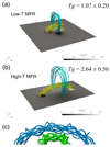 |
Fig. 1. Magnetic field models with low and high twists. Panels a, b represent the low-twist ( |
From each magnetic field model, we select 250 magnetic field lines to perform 1D hydrodynamic simulations, which are roughly uniformly distributed inside the magnetic flux rope. The localized heating is symmetrically imposed at the two footpoints of each flux tube, with the amplitude E1 = 1.0 × 10⁻² erg cm−3 s−1 (Xia et al. 2011). Similar to Karpen et al. (2003), the localized heating is ramped up linearly over 860 s and maintained thereafter. As the field-aligned gravity is not uniform and is flux-tube dependent, we compute its distribution according to the field line path, that is,  , where
  , s is the 1D coordinate along the field line, and
  is the unit tangential vector along the field line. Our atmospheric model is the same as in the previous simulations (Zhou et al. 2017a; Guo et al. 2021b), where the chromospheric temperature is about 6000 K, the density at the bottom is about 1.6 × 1014 cm−3, the coronal temperature is about 1 MK, and the thickness of the chromosphere is about 3 Mm. The atmosphere obtained in this way is not in thermodynamic equilibrium, and therefore we relax this initial state to a state both in force and energy equilibria in about 57 min.
3. Numerical results
3.1. Thread formation process and fine structures
We note that although the mean twist is significantly different between the two model flux ropes, both of them have three types of field lines, that is, nondipped, single-dipped, and multidipped, with different percentages. Figure 2 depicts the temporal evolution of the temperature distributions along three types of flux tubes in each model. The first row, Figs. 2a and b, shows the dynamic thread formation and evolution processes along the nondipped flux tubes in Low-T and High-T models. It is seen that the flux tubes without dips experience thermal nonequilibrium cycles, similar to previous works (Karpen et al. 2001; Froment et al. 2017), forming dynamic threads moving at high speed (Karpen et al. 2001). For the dynamic threads in the Low-T model (Fig. 2a), the period of the thread appearance is about 114.7 min, the thread lifetime is about 28.6 min, and the average velocity during the drainage is about 25.2 km s−1, which is consistent with observations (Zirker et al. 1998; Lin et al. 2003, 2005). For that in the High-T model (Fig. 2b), the period of the thermal nonequilibrium cycle is about 378.4 min, the thread lifetime is about 194.9 min, and the average velocity is roughly 7.9 km s−1. One can find that the period of the thermal nonequilibrium cycle increases with flux-tube length, which is consistent with the results of Luna et al. (2012). These small dynamic threads, referred to as “blobs” in Luna et al. (2012), are generally formed in nondipped arcades or shallow-dipped field lines and move downward to the chromosphere, forming counterstreaming flows. The second row of Fig. 2 illustrates the evolution of temperature along single-dipped flux tubes in the two models (Figs. 2c and d). In the Low-T model, only one thread is formed near the magnetic dip after the localized heating continues for 2.34 h. The thread is rather stable after quick damping of short-period oscillations, growing with time as the chromospheric evaporation continues. In contrast, in the High-T model, a thread is formed slightly away from the magnetic dip at t = 3.59 h, which then oscillates for several periods until it becomes stable at the magnetic dip. In addition, a second thread is formed at s = 50 Mm. This thread drains down to the footpoint, forming a dynamic thread as depicted in Fig. 2d. The formation of a second thread is consistent with previous works (Karpen et al. 2006; Xia et al. 2011; Guo et al. 2021b), but only takes places if the field line is long enough. In particular, longer field lines could delay the onset of catastrophic cooling (Guo et al. 2021b). Therefore, even with the same localized heating, the formation of prominence threads supported by highly twisted flux ropes requires more time than prominences supported by weakly twisted flux ropes. The third row of Fig. 2 shows the evolution of the temperature along double-dipped flux tubes in the two models, and two threads are formed in each model as seen in panels (e) and (f).
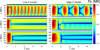 |
Fig. 2. Temporal evolution of the temperature distribution along a flux tube in the Low-T mode (left column) and the High-T model (right column), including dynamic threads (panels a, b), independently trapped threads (panels c, d), and magnetically connected threads (panels e, f). |
With the simulation results of all the 250 flux tubes in each model at the end of simulations (t ∼ 23 h), we can compile them and construct a 3D view of each prominence. In this paper, a prominence is referred to as a filament when viewed from above, which is similar to the terminology used to describe observations. Figures 3a–c display the distribution of the formed threads in the Low-T model viewed from different perspectives. As viewed from the top, we can see in Fig. 3a that although the photospheric magnetic PIL is along the x-axis, the filament spine, as indicated by the solid blue line, is inclined to the photospheric PIL (blue dashed line) by 17.1°. The filament spine is composed of many threads, and the thread orientation deviates from the filament spine by an angle ranging from 15° to 30°. For the side view along the y-axis in panel b, it is seen that all the threads pile up into an arch-shaped prominence, with the apex at an altitude of 16 Mm. For the end view along the x-axis in panel c, it is seen that the apparent width is quite large, and the two legs are overlapping. For comparison, we show the distribution of the formed threads in the High-T model from different perspectives in Figs. 3d–f. For the top view along the z-axis in panel d, we find that the filament spine is more parallel to the photospheric PIL. Moreover, the deviation angle between the threads and the filament spine is minimal near the middle of the flux ropes, and increases toward the footpoints for both cases. For the side view, the prominence can approximately outline the path of the flux rope axis in the High-T model (Fig. 3e). Regarding the end view, one can see that the prominence in the High-T model is composed of many short threads compared to the prominence height (Fig. 3f), reproducing a vertical thread-like structure.
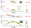 |
Fig. 3. Distribution of the prominence threads in different views. Panels a–c correspond to the top, side, and end views of the Low-T model; panels d–f correspond to the top, side, and end views of the High-T model. The blue solid lines in panels a, d represent the filament spines. The angles marked in blue represent those between the flux rope axes and filament spines, and the angles marked in red represent those between the thread orientations and filament spines. The insets show the maps of magnetic field in the photosphere, where the red solid lines represent the PILs. |
The cold and dense prominences are optically thick in the EUV range, that is, partial incident light is absorbed through the photoionization of the neutral hydrogen (H I), neutral helium (He I), and singly ionized helium (He I). Therefore, we solve the radiative transfer equation to synthesize the EUV radiation images (see also Zhao et al. 2019; Zhou et al. 2020; Jenkins & Keppens 2022), which is different from our previous optically thin modeling (Chen & Priest 2006). The solution to the radiative transfer equation (Rybicki et al. 1986) is as follows:
 (1)
(1)
where Iλ(τλ) is the measured specific radiation intensity at the wavelength λ, Iλ(0) is the incident intensity in the background, τλ is the total optical depth,  is the local optical thickness, Sλ = jλ/αλ is the source function, jλ is the emission coefficient, and αλ is the absorption coefficient. Among them, the optical depth and source function are highly dependent on the relative population of hydrogen and helium, and therefore we need to calculate the ionization degree with the Saha equation. The emission coefficient can then be calculated according to Formula (24) in Jenkins & Keppens (2022), and the absorption coefficient can be obtained from Formula (6) in Anzer & Heinzel (2005). Finally, similar to Jenkins & Keppens (2022), assuming an incident intensity Iλ(0), the transfer equation can be computed numerically, and the synthesized 171 Å images viewed from different directions are shown in Fig. 4.
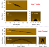 |
Fig. 4. Synthesized EUV 171 Å images in the two models. Panels a–c correspond to the top, side, and end views of the Low-T model; Panels d–f correspond to the top, side, and end views of the High-T model. |
For the top views, we find that the overall structure of the filament in the Low-T model resembles a rhombus, whereas that in the High-T model presents a stick-like morphology. Regarding the fine structures, it is seen that the filament spine is composed of right-bearing threads, which is in accordance with the chirality of the filament and the helicity of the supporting flux rope. Moreover, the edge of the filament spine in the High-T model is serrated while that in the Low-T model is smoother. Comparing the side views of the two models (Figs. 4b and e), we find that there are no obvious legs in the prominence supported by a low-twist flux rope. That is to say, these prominences would be manifested as being nearly detached from the solar surface. However, for the prominence supported by a highly twisted flux rope, its legs almost extend down all the way to the solar surface. For the end views along the flux rope axes (Figs. 4c and f), in the two models, cavities always appear on the top of the prominence condensations, which is consistent with 3D full MHD simulations of the flux-rope prominence formation (Xia et al. 2014a; Xia & Keppens 2016; Fan 2018; Fan & Liu 2019). In addition, we also find that the horn-like structures are much more evident in the Low-T model than in the High-T model.
3.2. Magnetic dip and thread characteristics
High-resolution observations reveal that prominences are composed of numerous separate fine-scale threads (Lin et al. 2005), which can be divided into dynamic threads, independently trapped threads, and magnetically connected threads (Guo et al. 2021b). These threads were found to move with velocities of roughly 15 ± 10 km s−1 (Engvold et al. 2004; Lin et al. 2005). The relationship between threads and magnetic dips is an important issue. Our pseudo-3D simulations provide a chance to study their relationship in detail.
As mentioned in Sect. 3.1, although the mean twist is 1.07 turns in the Low-T model and 2.64 turns in the High-T model, both models have nondipped field lines, single-dipped field lines, and multidipped field lines. Figures 5a and b show the fractions of the field lines without dips, with a single dip, and with multiple dips in the two models. One can see that whereas most field lines (78%) are nondipped in the Low-T model, only 26.4% of the field lines are nondipped in the High-T model. In particular, 48.4% of the field lines possess more than one dip in the High-T model. We also calculate the fractions of different types of threads, which are shown in Figs. 5c and d. It is found that 82.8% of the threads are dynamic threads in the Low-T model, and others (17.2%) are quasi-static threads oscillating near magnetic dips. On the other hand, 60.6% of the threads are quasi-static threads in the High-T model.
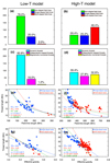 |
Fig. 5. Statistical results of magnetic dip and thread characteristics in the Low-T (left column) and High-T (right column) models. Panels a, b: fractions of different types of magnetic field lines; panels c, d: fractions of different types of threads; panels e, f: scatter plots of the field-line length versus mean thread length; panels g, h: scatter plots of the effective gravity of the dip versus the thread length. The blue solid circles denote the single-dipped cases, and the red solid circles denote the multidipped cases. The dashed lines marked in blue, red, and green display the fittings to single-dipped cases, multidipped cases, and all data points, respectively. |
Thread length is another observational feature that can shed light on the magnetic structure of the supporting field lines of prominences (Karpen et al. 2003; Zhou et al. 2014; Guo et al. 2021b). Rather than investigating the relationship between thread length and the parameters of the magnetic dip, as done by Zhou et al. (2014), we intend to check the relationship between the thread length and the total length of the magnetic field line for simplicity. For this purpose, we selected the quasi-static threads, and the thread length in the multidip field lines is the averaged length of multiple threads. In Figs. 5e–f, we display the dependence of thread length (Lt) on field-line length (Lf). Despite scattering, there is a tendency for the thread length to decrease with field-line length. We divide the data points into single-dipped threads (blue) and multidipped threads (red), and then fit the Lt − Lf relationships with power-law functions,  , for the three groups of data, that is, single-dipped threads (blue), multidipped threads (red), and all threads (green). For the Low-T model in Fig. 5e, the corresponding fitting functions are
  ,
,  , and
, and  , respectively, where Lt and Lf are in units of megameters (Mm). And the corresponding Spearman correlation coefficients are −0.51, −0.50, and −0.60, respectively. Regarding the High-T model in Fig. 5f, the corresponding fitting functions are
  ,
,  , and
, and  , with the correlation coefficients of −0.83, −0.79, and −0.89, respectively.
It is well known that for a vertical flux tube, the typical length of a plasma structure is the scale height, which is related to gravity. By analogy, the length of a prominence thread along a magnetic dip might be related to effective gravity, which is defined as  . As demonstrated by Guo et al. (2021b), such a single parameter can reflect the magnetic dip configuration comprehensively. Figures 5g–h reveal that the thread length decreases with effective gravity, meaning that longer threads are likely to exist in longer and shallower magnetic dips, which is consistent with Zhou et al. (2014). The relationship between thread length and the effective gravity ge is fitted with a linear function. In the Low-T model, the corresponding fitting functions are Lt = −17.12ge + 22.71, Lt = −31.80ge + 25.97, and Lt = −24.81ge + 24.84 for the single-dipped threads, multidipped threads, and all threads, respectively. The corresponding correlation coefficients are −0.64, −0.92, and −0.73, respectively. In the High-T model, the fitting functions are Lt = −45.11ge + 31.54, Lt = −101.55ge + 53.64, and Lt = −73.69ge + 40.85 for the single-dipped threads, multidipped threads, and all threads, respectively. The corresponding correlation coefficients are −0.89, −0.77, and −0.86, respectively. We find that thread length is better correlated with effective gravity than with field-line length in the Low-T model, but the opposite is true for the High-T model. The reason is that in the High-T model, magnetically connected threads account for a significant proportion. Mutual interactions among the multiple dips along an individual field line reduce the role of the local dip geometry.
4. Discussions
4.1. Morphological differences between prominences with different twists
Magnetic twist is an important parameter of magnetic structures, describing how many times a bunch of field lines winds around an axis (Liu et al. 2016). This parameter plays a significant role in predicting solar eruptions and our understanding of the dynamics of coronal mass ejections (CMEs; Chen 2011). However, the estimate of magnetic twist is nontrivial because it relies on coronal magnetic extrapolations, which are an ill-posed boundary-value problem based on noisy vector magnetic field on the solar surface. As prominences are usually regarded as the tracers of coronal sheared/twisted magnetic structures, their morphology might reflect the twisting properties of their magnetic structures. In this paper, we explored the morphological differences between two simulated prominences with different twists. The morphological features include (1) how many threads are quasi-static and how many threads are dynamic; (2) the thread length; and (3) whether the prominence is detached from the solar surface.
Observations indicate that some threads are quasi-static, oscillating near the equilibrium positions (Jing et al. 2003), and other threads are dynamic, moving from one polarity to the other as siphon flows (Wang 1999; Zou et al. 2016). In our simulations, both types of threads exist in the simulated prominences. In the flux rope system with a low twist, the percentage of quasi-static threads is about 17%, with the remaining 83% being dynamic threads. On the contrary, in the flux rope system with a high twist, the percentage of quasi-static threads, including independently trapped threads and magnetically connected threads, is about 61%, with the remaining 39% being dynamic threads. It is seen that the prominences supported by low-twist flux ropes are mainly composed of short-lived dynamic threads, while the prominences supported by high-twist flux ropes are mainly composed of long-lived quasi-static threads. Therefore, the counterstreamings in a weakly twisted flux rope are composed mainly of alternative unidirectional flows (Zou et al. 2017), while the counterstreamings in a highly twisted flux rope are composed mainly of oscillating threads around magnetic dips (Chen et al. 2014; Zhou et al. 2020). Both types of threads exist in prominences, and so the counterstreamings of prominences might be composed of both prominence longitudinal oscillations and unidirectional flows, with the proportion being determined by the twist of the supporting flux rope. In addition, in the prominence supported by a high-twist flux rope, there are many short magnetically connected thread pairs, that is, thread pairs connected by double-dipped field lines, which tend to present drastically decaying and decayless oscillations for one thread and the other, respectively (Zhou et al. 2017a; Zhang et al. 2017).
The thread length is also systematically different in flux ropes with different twists. First, the magnetically connected threads that exist widely in prominences supported by the high-twist flux rope are usually shorter than independently trapped threads. As a result, the vertical piling of these short threads might resemble the observed vertical-like threads in quiescent prominences (Berger et al. 2008; Mackay et al. 2010; Schmieder et al. 2010, 2014). Second, while shorter dips host shorter threads (Zhou et al. 2014), we find that magnetically connected threads tend to be much shorter. As seen from the synthesized EUV images in Fig. 4d, some longer threads stand out from shorter threads, and these longer threads manifest as prominence barbs. Similar to the dynamic barbs (Ouyang et al. 2020), these barbs do not correspond to prominence feet that extend down to the solar surface.
Observations have revealed that some prominences are totally suspended in the corona, whereas others possess two or more legs extending down to the solar surface. Our simulations indicate that the prominence in the high-twist flux rope is nearly attached to the solar surface, but the prominence in the low-twist flux rope is detached. Our results might imply that those detached prominences are probably supported by low-twist flux ropes, and those attached prominences with two endpoints near the solar chromosphere are supported by high-twist flux ropes. The simulation results in our Low-T model are similar to those in the simulation of Luna et al. (2012), wherein the magnetic twist is about one turn. In both papers, the threads are almost horizontal, and the prominences are detached from the solar surface. This might imply that there is no sharp dividing line between sheared arcades and weakly twisted flux ropes.
When viewed along the spine direction, some prominences show horn-like structures, which are intimately related coronal cavities (Schmit et al. 2013; Schmit & Gibson 2013). Our simulations nicely reproduced the horn-like structures. Comparing the end views of the low-twist and high-twist flux ropes in Figs. 4c and f, we can find that the horns are much more evident in the Low-T model than in the High-T model. We tentatively suggest that the clearer prominence horns are a signature of less twisted magnetic field lines.
Despite all these differences, the two models reveal some common features in the synthesized prominences. For example, the deviation angle between the threads and the prominence axis ranges from 10° to 35°, which is consistent with observations (Hanaoka & Sakurai 2017). On the other hand, our simulations show that such a deviation angle increases from the middle of the prominence spine to the two endpoints, which does not seem to be a ubiquitous feature in observations. It appears that the variation of the deviation angle depends on the magnetic configuration model, and the monotonic variation from the middle of the spine to the endpoints might be an intrinsic property of the TDm flux-rope model, which has a low-twist core and a high-twist outer shell (Guo et al. 2021a). However, these fnidings suggest that we might be able to utilize the distribution of the thread deviation angle to diagnose the radial distribution of the magnetic twist in the flux rope. As the twist profile may affect the threshold of the kink instability (Baty 2001), the distribution of the thread deviation angles can serve as an important proxy for future space weather forecasting.
4.2. Relationship between prominences and flux ropes
A statistical study indicated that whereas ∼11% of prominences are supported by sheared magnetic arcades, ∼89% are supported by flux ropes (Ouyang et al. 2017). Hence, in the majority of cases the magnetic structure of prominences is a flux rope, in particular for the quiescent prominences. However, the spatial relationship between a flux rope and a prominence is unclear (Zhou et al. 2017b), and is generally assumed that the dense plasmas of a prominence are situated at the magnetic dips, and are therefore located on the underside of a flux rope (Rust & Kumar 1994).
In order to check the spatial relationship between prominences and flux ropes, we overlaid the simulated prominence with the magnetic flux rope in the Low-twist model together. The result is shown in Fig. 6. Here, we note that the prominence is characterized by the plasma, the temperature of which is below 20 000 K, and the outer boundary of the flux rope is determined by calculating the squashing factor of magnetic connectivity (Q value). Here the outer boundary of the flux rope corresponds to Q ≫ 2 (Priest & Démoulin 1995; Titov et al. 2002), that is, it corresponds to magnetic quasi-separatrix layers (QSLs). It is seen from Fig. 6 that not only does the prominence deviate from the flux-rope axis, but also the prominence condensations do not fully fill the lower half of the flux rope. We also see that in the Low-twist model, the dense plasmas of the prominence occupy only the lower quarter of the radial extent of the flux rope. Therefore, we have to be careful when taking a prominence as the tracer of a magnetic flux rope.
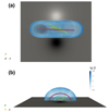 |
Fig. 6. Simulated prominence condensations and the QSL that wraps the flux rope in the Low-T model, where the green isosurface represents the simulated prominence, the blue isosurfaces represent the flux ropes, and the red lines indicate the axes of flux ropes. Panels a, b represent the top and side views, respectively. |
Another caveat is that prominences are often claimed to be located above the magnetic polarity inversion line of the photospheric magnetogram (Mackay et al. 2010). However, according to our simulations, prominence spines are skewed from the photospheric PILs and cospatial with the coronal PILs, as shown in Fig. 7. It should be pointed out that the filament threads in our simulations are located in magnetic dips. However, the troughs of these dips correspond to the local PIL at the bottom of the flux rope in the corona, not the PIL on the photosphere. Depending on the complexity of the magnetic configuration, the coronal PILs and the photospheric PILs might be roughly cospatial or might be skewed significantly.
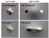 |
Fig. 7. Spatial relationship between the PILs and filaments in the Low-T (panels a, c) and High-T (panels b, d) models, where the red solid lines denote the PILs, and the green isosurfaces represent the simulated filaments, which are overlaid on the magnetograms (gray scale). The first row illustrates the photospheric magnetograms, and the bottom row illustrates the coronal magnetograms at the bottom of the flux rope (10 Mm for the Low-T model and 31 Mm for the High-T model). |
5. Summary
In this paper, we explore the differences in the prominence fine structure characteristics between two flux ropes with different twists, one with low twist, and the other with high twist. In summary, our simulations lead to the following results:
-
The types of threads are different in the two models, which might produce different dynamic behaviors. In the low-twist model, the majority of the threads are short-lived dynamic threads (83%), forming high-speed flows inside the filament. However, for the high-twist model, quasi-stationary threads account for about 61% and generally present longitudinal oscillations around the dips.
-
The thread lengths are different in the two models, which might produce morphological differences. First, the piling of short magnetically connected threads that widely exist in prominences supported by high-twist flux ropes might resemble the observed vertical-like structures. Second, elongated threads in single-dipped field lines probably stand out from short magnetically connected threads, manifesting as filament barbs without feet.
-
The filament spine is not cospatial with its supporting flux rope axis and PIL in the photospheric magnetogram, especially for the low-twist flux rope model. We find that not only does the prominence deviate from the flux rope axis in height, but also the prominence condensations do not fully fill the lower half of the flux rope. Only the lowest quarter of the radial extent of the flux rope is filled with cold plasmas in our simulations. Therefore, one has to be careful when taking a prominence as the tracer of a magnetic flux rope.
It is noted that our simulations also have some drawbacks. First, these simulations are based on the evaporation–condensation model, whereas other models of prominence formation might influence the appearance of the simulated prominence. For example, for the injection model, cold material injected from the chromosphere is likely to experience expansion, which might form elongated threads (Huang et al. 2021). Second, our simulation results highly depend on the magnetic configuration of the TDm model. In the future, we will consider the pseudo-3D model based on the NLFFF extrapolations and data-driven models from observations. Third, we ignored the effects of the prominences on the magnetic structures. However, the magnetic field might be deformed by the prominence weight when plasma δ (the ratio of the gravity to the magnetic pressure) is large enough (Zhou et al. 2018). In reality, the heating at the footpoint is probably very complex; for example, the turbulent heating (Zhou et al. 2020) or the heating related to the magnetic fields (Yang et al. 2018). However, in this paper, to emphasize the effects of the magnetic configuration, we only considered a simplified and robust pattern (continuous and steady heating independent of the magnetic fields). Nevertheless, the above findings deepen our understanding of the relationships between prominences and their supporting magnetic structures, which provides a scientific basis for studying the magnetic structures of prominences before the eruption. We also expect high-resolution, 3D, full-MHD simulations in the future to reinforce our conclusions.
Acknowledgments
This research was supported by National Key Research and Development Program of China (2020YFC2201200), NSFC (12127901, 11961131002, 11773016, and 11533005), and Belgian FWO-NSFC project G0E9619N. The numerical calculations in this paper were performed in the cluster system of the High Performance Computing Center (HPCC) of Nanjing University.
References
- An, C. H., Bao, J. J., Wu, S. T., & Suess, S. T. 1988, Sol. Phys., 115, 93 [Google Scholar]
- Antiochos, S. K., MacNeice, P. J., Spicer, D. S., & Klimchuk, J. A. 1999, ApJ, 512, 985 [Google Scholar]
- Anzer, U., & Heinzel, P. 2005, ApJ, 622, 714 [Google Scholar]
- Baty, H. 2001, A&A, 367, 321 [NASA ADS] [CrossRef] [EDP Sciences] [Google Scholar]
- Berger, M. A., & Prior, C. 2006, J. Phys. A Math. Gen., 39, 8321 [Google Scholar]
- Berger, T. E., Shine, R. A., Slater, G. L., et al. 2008, ApJ, 676, L89 [Google Scholar]
- Bommier, V., & Leroy, J. L. 1998, in IAU Colloq. 167: New Perspectives on Solar Prominences, eds. D. F. Webb, B. Schmieder, & D. M. Rust, ASP Conf. Ser., 150, 434 [NASA ADS] [Google Scholar]
- Bommier, V., Landi Degl’Innocenti, E., Leroy, J.-L., & Sahal-Brechot, S. 1994, Sol. Phys., 154, 231 [NASA ADS] [CrossRef] [Google Scholar]
- Braginskii, S. I. 1965, Rev. Plasma Phys., 1, 205 [Google Scholar]
- Chen, P. F. 2011, Liv. Rev. Sol. Phys., 8, 1 [Google Scholar]
- Chen, P. F., & Priest, E. R. 2006, Sol. Phys., 238, 313 [Google Scholar]
- Chen, P. F., Harra, L. K., & Fang, C. 2014, ApJ, 784, 50 [NASA ADS] [CrossRef] [Google Scholar]
- Chen, P.-F., Xu, A.-A., & Ding, M.-D. 2020, Res. Astron. Astrophys., 20, 166 [Google Scholar]
- DeVore, C. R., & Antiochos, S. K. 2000, ApJ, 539, 954 [NASA ADS] [CrossRef] [Google Scholar]
- DeVore, C. R., Antiochos, S. K., & Aulanier, G. 2005, ApJ, 629, 1122 [NASA ADS] [CrossRef] [Google Scholar]
- Engvold, O. 2004, in Multi-Wavelength Investigations of Solar Activity, eds. A. V. Stepanov, E. E. Benevolenskaya, & A. G. Kosovichev, IAU Symp., 223, 187 [NASA ADS] [Google Scholar]
- Engvold, O. 2015, in Description and Classification of Prominences, eds. J.-C. Vial, & O. Engvold, Astrophys. Space Sci. Lib., 415, 31 [NASA ADS] [Google Scholar]
- Fan, Y. 2001, ApJ, 554, L111 [NASA ADS] [CrossRef] [Google Scholar]
- Fan, Y. 2018, ApJ, 862, 54 [Google Scholar]
- Fan, Y. 2020, ApJ, 898, 34 [Google Scholar]
- Fan, Y., & Liu, T. 2019, Front. Astron. Space Sci., 6, 27 [NASA ADS] [CrossRef] [Google Scholar]
- Froment, C., Auchère, F., Aulanier, G., et al. 2017, ApJ, 835, 272 [Google Scholar]
- Guo, Y., Schmieder, B., Démoulin, P., et al. 2010, ApJ, 714, 343 [Google Scholar]
- Guo, Y., Xia, C., & Keppens, R. 2016a, ApJ, 828, 83 [NASA ADS] [CrossRef] [Google Scholar]
- Guo, Y., Xia, C., Keppens, R., & Valori, G. 2016b, ApJ, 828, 82 [NASA ADS] [CrossRef] [Google Scholar]
- Guo, Y., Xu, Y., Ding, M. D., et al. 2019, ApJ, 884, L1 [NASA ADS] [CrossRef] [Google Scholar]
- Guo, J. H., Ni, Y. W., Qiu, Y., et al. 2021a, ApJ, 917, 81 [NASA ADS] [CrossRef] [Google Scholar]
- Guo, J. H., Zhou, Y. H., Guo, Y., et al. 2021b, ApJ, 920, 131 [NASA ADS] [CrossRef] [Google Scholar]
- Hanaoka, Y., & Sakurai, T. 2017, ApJ, 851, 130 [NASA ADS] [CrossRef] [Google Scholar]
- Hood, A. W., & Priest, E. R. 1979, Sol. Phys., 64, 303 [NASA ADS] [CrossRef] [Google Scholar]
- Huang, C. J., Guo, J. H., Ni, Y. W., Xu, A. A., & Chen, P. F. 2021, ApJ, 913, L8 [CrossRef] [Google Scholar]
- Jenkins, J. M., & Keppens, R. 2022, Nat. Astron., 6, 942 [NASA ADS] [CrossRef] [Google Scholar]
- Jiang, C., Wu, S. T., Feng, X., & Hu, Q. 2014, ApJ, 786, L16 [NASA ADS] [CrossRef] [Google Scholar]
- Jibben, P., Reeves, K., & Su, Y. 2016, Front. Astron. Space Sci., 3, 10 [NASA ADS] [CrossRef] [Google Scholar]
- Jing, J., Lee, J., Spirock, T. J., et al. 2003, ApJ, 584, L103 [NASA ADS] [CrossRef] [Google Scholar]
- Karpen, J. T., Antiochos, S. K., Hohensee, M., Klimchuk, J. A., & MacNeice, P. J. 2001, ApJ, 553, L85 [Google Scholar]
- Karpen, J. T., Antiochos, S. K., Klimchuk, J. A., & MacNeice, P. J. 2003, ApJ, 593, 1187 [NASA ADS] [CrossRef] [Google Scholar]
- Karpen, J. T., Antiochos, S. K., & Klimchuk, J. A. 2006, ApJ, 637, 531 [Google Scholar]
- Keppens, R., Teunissen, J., Xia, C., & Porth, O. 2020, ArXiv e-prints [arXiv:2004.03275] [Google Scholar]
- Kippenhahn, R., & Schlüter, A. 1957, ZAp, 43, 36 [NASA ADS] [Google Scholar]
- Kuperus, M., & Raadu, M. A. 1974, A&A, 31, 189 [NASA ADS] [Google Scholar]
- Leroy, J. L., Bommier, V., & Sahal-Brechot, S. 1984, A&A, 131, 33 [Google Scholar]
- Lin, Y., Engvold, O. R., & Wiik, J. E. 2003, Sol. Phys., 216, 109 [NASA ADS] [CrossRef] [Google Scholar]
- Lin, Y., Engvold, O., Rouppe van der Voort, L., Wiik, J. E., & Berger, T. E. 2005, Sol. Phys., 226, 239 [Google Scholar]
- Liu, R., Kliem, B., Titov, V. S., et al. 2016, ApJ, 818, 148 [Google Scholar]
- Liu, J., Wang, Y., & Erdélyi, R. 2019, Front. Astron. Space Sci., 6, 44 [NASA ADS] [CrossRef] [Google Scholar]
- Low, B. C. 2015, SCPMA, 58, 5626 [Google Scholar]
- Low, B. C., & Lou, Y. Q. 1990, ApJ, 352, 343 [NASA ADS] [CrossRef] [Google Scholar]
- Luna, M., Karpen, J. T., & DeVore, C. R. 2012, ApJ, 746, 30 [Google Scholar]
- Luna, M., Su, Y., Schmieder, B., Chandra, R., & Kucera, T. A. 2017, ApJ, 850, 143 [NASA ADS] [CrossRef] [Google Scholar]
- Mackay, D. H., Karpen, J. T., Ballester, J. L., Schmieder, B., & Aulanier, G. 2010, Space Sci. Rev., 151, 333 [Google Scholar]
- Mackay, D. H., Schmieder, B., López Ariste, A., & Su, Y. 2020, A&A, 637, A3 [NASA ADS] [CrossRef] [EDP Sciences] [Google Scholar]
- Martin, S. F. 1998, Sol. Phys., 182, 107 [Google Scholar]
- Ni, Y. W., Guo, J. H., Zhang, Q. M., et al. 2022, A&A, 663, A31 [NASA ADS] [CrossRef] [EDP Sciences] [Google Scholar]
- Ouyang, Y., Zhou, Y. H., Chen, P. F., & Fang, C. 2017, ApJ, 835, 94 [NASA ADS] [CrossRef] [Google Scholar]
- Ouyang, Y., Chen, P. F., Fan, S. Q., Li, B., & Xu, A. A. 2020, ApJ, 894, 64 [Google Scholar]
- Patsourakos, S., Vourlidas, A., Török, T., et al. 2020, Space Sci. Rev., 216, 131 [Google Scholar]
- Priest, E. R., & Démoulin, P. 1995, J. Geophys. Res., 100, 23443 [NASA ADS] [CrossRef] [Google Scholar]
- Romano, P., Contarino, L., & Zuccarello, F. 2003, Sol. Phys., 214, 313 [Google Scholar]
- Rust, D. M., & Kumar, A. 1994, Sol. Phys., 155, 69 [NASA ADS] [CrossRef] [Google Scholar]
- Rybicki, G. B., & Lightman, A. P. 1986, in Radiative Processes in Astrophysics, eds. G. B. Rybicki, & A. P. Lightman [Google Scholar]
- Schmieder, B., Chandra, R., Berlicki, A., & Mein, P. 2010, A&A, 514, A68 [CrossRef] [EDP Sciences] [Google Scholar]
- Schmieder, B., Tian, H., Kucera, T., et al. 2014, A&A, 569, A85 [NASA ADS] [CrossRef] [EDP Sciences] [Google Scholar]
- Schmit, D. J., & Gibson, S. 2013, ApJ, 770, 35 [NASA ADS] [CrossRef] [Google Scholar]
- Schmit, D. J., Gibson, S., Luna, M., Karpen, J., & Innes, D. 2013, ApJ, 779, 156 [NASA ADS] [CrossRef] [Google Scholar]
- Su, Y., van Ballegooijen, A., McCauley, P., et al. 2015, ApJ, 807, 144 [NASA ADS] [CrossRef] [Google Scholar]
- Tandberg-Hanssen, E. 1995, The Nature of Solar Prominences, 199 (Dordrecht: Kluwer Academic Publishers) [Google Scholar]
- Titov, V. S., & Démoulin, P. 1999, A&A, 351, 707 [NASA ADS] [Google Scholar]
- Titov, V. S., Hornig, G., & Démoulin, P. 2002, J. Geophys. Res. (Space Phys.), 107, 1164 [Google Scholar]
- Titov, V. S., Török, T., Mikic, Z., & Linker, J. A. 2014, ApJ, 790, 163 [NASA ADS] [CrossRef] [Google Scholar]
- Titov, V. S., Downs, C., Mikić, Z., et al. 2018, ApJ, 852, L21 [NASA ADS] [CrossRef] [Google Scholar]
- Török, T., & Kliem, B. 2005, ApJ, 630, L97 [Google Scholar]
- Török, T., Kliem, B., & Titov, V. S. 2004, A&A, 413, L27 [NASA ADS] [CrossRef] [EDP Sciences] [Google Scholar]
- van Ballegooijen, A. A. 2004, ApJ, 612, 519 [NASA ADS] [CrossRef] [Google Scholar]
- Vrsnak, B., Ruzdjak, V., & Rompolt, B. 1991, Sol. Phys., 136, 151 [NASA ADS] [CrossRef] [Google Scholar]
- Wang, Y. M. 1999, ApJ, 520, L71 [Google Scholar]
- Wang, Y., Zhuang, B., Hu, Q., et al. 2016, J. Geophys. Res. (Space Phys.), 121, 9316 [NASA ADS] [CrossRef] [Google Scholar]
- Wheatland, M. S., Sturrock, P. A., & Roumeliotis, G. 2000, ApJ, 540, 1150 [Google Scholar]
- Wiegelmann, T. 2004, Sol. Phys., 219, 87 [NASA ADS] [CrossRef] [Google Scholar]
- Wiegelmann, T., & Sakurai, T. 2021, Liv. Rev. Sol. Phys., 18, 1 [NASA ADS] [CrossRef] [Google Scholar]
- Xia, C., & Keppens, R. 2016, ApJ, 823, 22 [Google Scholar]
- Xia, C., Chen, P. F., Keppens, R., & van Marle, A. J. 2011, ApJ, 737, 27 [NASA ADS] [CrossRef] [Google Scholar]
- Xia, C., Keppens, R., Antolin, P., & Porth, O. 2014a, ApJ, 792, L38 [Google Scholar]
- Xia, C., Keppens, R., & Guo, Y. 2014b, ApJ, 780, 130 [Google Scholar]
- Xia, C., Teunissen, J., El Mellah, I., Chané, E., & Keppens, R. 2018, ApJ, 234, S30 [Google Scholar]
- Yang, W. H., Sturrock, P. A., & Antiochos, S. K. 1986, ApJ, 309, 383 [NASA ADS] [CrossRef] [Google Scholar]
- Yang, K. E., Longcope, D. W., Ding, M. D., & Guo, Y. 2018, Nat. Commun., 9, 692 [NASA ADS] [CrossRef] [Google Scholar]
- Zhang, Q. M., Chen, P. F., Xia, C., & Keppens, R. 2012, A&A, 542, A52 [NASA ADS] [CrossRef] [EDP Sciences] [Google Scholar]
- Zhang, Q. M., Li, T., Zheng, R. S., Su, Y. N., & Ji, H. S. 2017, ApJ, 842, 27 [CrossRef] [Google Scholar]
- Zhang, Q. M., Guo, J. H., Tam, K. V., & Xu, A. A. 2020, A&A, 635, A132 [NASA ADS] [CrossRef] [EDP Sciences] [Google Scholar]
- Zhao, X., Xia, C., Van Doorsselaere, T., Keppens, R., & Gan, W. 2019, ApJ, 872, 190 [Google Scholar]
- Zhou, Y.-H., Chen, P.-F., Zhang, Q.-M., & Fang, C. 2014, Res. Astron. Astrophys., 14, 581 [Google Scholar]
- Zhou, Y.-H., Zhang, L.-Y., Ouyang, Y., Chen, P. F., & Fang, C. 2017a, ApJ, 839, 9 [NASA ADS] [CrossRef] [Google Scholar]
- Zhou, Z., Zhang, J., Wang, Y., Liu, R., & Chintzoglou, G. 2017b, ApJ, 851, 133 [Google Scholar]
- Zhou, Y.-H., Xia, C., Keppens, R., Fang, C., & Chen, P. F. 2018, ApJ, 856, 179 [Google Scholar]
- Zhou, Y. H., Chen, P. F., Hong, J., & Fang, C. 2020, Nat. Astron., 4, 994 [NASA ADS] [CrossRef] [Google Scholar]
- Zirker, J. B., Engvold, O., & Martin, S. F. 1998, Nature, 396, 440 [Google Scholar]
- Zou, P., Fang, C., Chen, P. F., et al. 2016, ApJ, 831, 123 [NASA ADS] [CrossRef] [Google Scholar]
- Zou, P., Fang, C., Chen, P. F., Yang, K., & Cao, W. 2017, ApJ, 836, 122 [NASA ADS] [CrossRef] [Google Scholar]
All Figures
|
Fig. 1. Magnetic field models with low and high twists. Panels a, b represent the low-twist ( |
| In the text | |
|
Fig. 2. Temporal evolution of the temperature distribution along a flux tube in the Low-T mode (left column) and the High-T model (right column), including dynamic threads (panels a, b), independently trapped threads (panels c, d), and magnetically connected threads (panels e, f). |
| In the text | |
|
Fig. 3. Distribution of the prominence threads in different views. Panels a–c correspond to the top, side, and end views of the Low-T model; panels d–f correspond to the top, side, and end views of the High-T model. The blue solid lines in panels a, d represent the filament spines. The angles marked in blue represent those between the flux rope axes and filament spines, and the angles marked in red represent those between the thread orientations and filament spines. The insets show the maps of magnetic field in the photosphere, where the red solid lines represent the PILs. |
| In the text | |
|
Fig. 4. Synthesized EUV 171 Å images in the two models. Panels a–c correspond to the top, side, and end views of the Low-T model; Panels d–f correspond to the top, side, and end views of the High-T model. |
| In the text | |
|
Fig. 5. Statistical results of magnetic dip and thread characteristics in the Low-T (left column) and High-T (right column) models. Panels a, b: fractions of different types of magnetic field lines; panels c, d: fractions of different types of threads; panels e, f: scatter plots of the field-line length versus mean thread length; panels g, h: scatter plots of the effective gravity of the dip versus the thread length. The blue solid circles denote the single-dipped cases, and the red solid circles denote the multidipped cases. The dashed lines marked in blue, red, and green display the fittings to single-dipped cases, multidipped cases, and all data points, respectively. |
| In the text | |
|
Fig. 6. Simulated prominence condensations and the QSL that wraps the flux rope in the Low-T model, where the green isosurface represents the simulated prominence, the blue isosurfaces represent the flux ropes, and the red lines indicate the axes of flux ropes. Panels a, b represent the top and side views, respectively. |
| In the text | |
|
Fig. 7. Spatial relationship between the PILs and filaments in the Low-T (panels a, c) and High-T (panels b, d) models, where the red solid lines denote the PILs, and the green isosurfaces represent the simulated filaments, which are overlaid on the magnetograms (gray scale). The first row illustrates the photospheric magnetograms, and the bottom row illustrates the coronal magnetograms at the bottom of the flux rope (10 Mm for the Low-T model and 31 Mm for the High-T model). |
| In the text | |
Current usage metrics show cumulative count of Article Views (full-text article views including HTML views, PDF and ePub downloads, according to the available data) and Abstracts Views on Vision4Press platform.
Data correspond to usage on the plateform after 2015. The current usage metrics is available 48-96 hours after online publication and is updated daily on week days.
Initial download of the metrics may take a while.