| Issue |
A&A
Volume 591, July 2016
|
|
|---|---|---|
| Article Number | A51 | |
| Number of page(s) | 22 | |
| Section | Extragalactic astronomy | |
| DOI | https://doi.org/10.1051/0004-6361/201527705 | |
| Published online | 10 June 2016 | |
Simulations of ram-pressure stripping in galaxy-cluster interactions
1
Institut für Astro- und Teilchenphysik Universität Innsbruck,
Technikerstrasse 25/8,
6020
Innsbruck,
Austria
e-mail:
dominik.steinhauser@uibk.ac.at
2
Heidelberger Institut für Theoretische Studien,
Schloss-Wolfsbrunnenweg 35,
69118
Heidelberg,
Germany
3
Zentrum für Astronomie der Universität Heidelberg,
Astronomisches Recheninstitut, Mönchhofstr.
12-14, 69120
Heidelberg,
Germany
Received: 5 November 2015
Accepted: 7 March 2016
Context. Observationally, the quenching of star-forming galaxies appears to depend both on their mass and environment. The exact cause of the environmental dependence is still poorly understood, yet semi-analytic models (SAMs) of galaxy formation need to parameterise it to reproduce observations of galaxy properties.
Aims. In this work, we use hydrodynamical simulations to investigate the quenching of disk galaxies through ram-pressure stripping (RPS) as they fall into galaxy clusters with the goal of characterising the importance of this effect for the reddening of disk galaxies. In particular, we compare our findings for the mass loss and evolution of the star formation rate in our simulations with prescriptions commonly employed in SAMs. We also analyse the gaseous wake of the galaxy, focusing on gas mixing and metal enrichment of the intracluster medium (ICM).
Methods. Our set-up employs a live model of a galaxy cluster that interacts with infalling disk galaxies on different orbits. We use the moving-mesh code AREPO, augmented with a special refinement strategy to yield high resolution around the galaxy on its way through the cluster in a computationally efficient way. Cooling, star formation, and stellar feedback are included according to a simple sub-resolution model. Stellar light maps and the evolution of galaxy colours are computed with the stellar synthesis code FSPS to draw conclusions about quenching timescales of our model galaxies.
Results. We find that the stripping models employed in current SAMs often differ substantially from our direct simulations. In most cases, the actual stripping radius of the simulated disk galaxies is larger than assumed in the SAMs, corresponding to an over prediction of the mass loss in SAMs. As long as the disk is not completely stripped in peaks of RPS during pericentre passage, some gas that remains bound to the galaxies is redistributed to the outer parts of disks as soon as the ram pressure becomes weaker again, an effect that is not captured in simplified treatements of RPS. Star formation in our model galaxies is quenched mainly because the hot gas halo is stripped, depriving the galaxy of its gas supply. The cold gas disk is only stripped completely in extreme cases, leading to full quenching and significant reddening on a very short timescale. Depending on the inclination angle, this can light up a galaxy for a few hundred Myrs until all of the gas is stripped or consumed and star formation drops to almost zero, suggesting a typical quenching timescale of ~200 Myr. On the other hand, galaxies experiencing only mild ram pressure actually show an enhanced star formation rate that is consistent with observations. Stripped gas in the wake is mixed efficiently with intracluster gas already a few tens of kpc behind the disk, and this gas is free of residual star formation.
Key words: galaxies: evolution / galaxies: clusters: general / methods: numerical / galaxies: interactions / galaxies: star formation
© ESO, 2016
1. Introduction
Galaxy surveys have shown that the quenching of disk galaxies mainly depends on their mass and environment (Peng et al. 2010; Schawinski et al. 2014). However, the question of the physical mechanisms behind quenching still persists, and especially the environmental dependence, which also gives rise to phenomena such as “galaxy conformity” (Weinmann et al. 2006; Kauffmann et al. 2013), is not well understood. Since the density of the environment seems to play an important role, and the merger cross section is small in galaxy clusters owing to the high relative velocity dispersion, classic ram-pressure stripping (RPS, e.g. Gunn & Gott 1972), the removal and possible compression of parts of the gas disk due to interaction with the intracluster medium (ICM), remains one of the main candidates responsible for environmental quenching of disk galaxies. Indirect evidence for RPS in action are asymmetries and truncated radial density profiles (e.g. Merluzzi et al. 2013; Chung et al. 2009) observed in many systems, which cannot be easily reproduced by pure “starvation” scenarios (the removal of the extended gas reservoir that refuels the disk with gas available for star formation (SF); e.g. Larson et al. 1980). Furthermore, starvation cannot modify the colours of galaxies on sufficiently short timescales, unlike RPS (Boselli et al. 2009).
It hence is plausible that the evolution of a galaxy strongly depends on the strength of ram pressure (RP) it experiences. Observations (e.g. Boselli et al. 1997; Vollmer et al. 2001a; Scott et al. 2010) often suggest only rather mild RPS acting on galaxies with atomic hydrogen only partly removed and slightly displaced from the stellar disk. Correspondingly, SF is slowly quenched and only slightly enhanced at the compressed interface between the intracluster and intrastellar media. High resolution observations (e.g. Abramson & Kenney 2014) have shown that dense gas clouds can stay in place even beyond the stripping radius, whereas the surrounding, diffuse and less dense gas is stripped. However, those clouds continue to form stars at a very low rate, contributing at most a few percent of the pre-stripping SFR, meaning that SF effectively ceases as soon as the gas with low density is stripped.
On the other hand, in very massive clusters (with ρ ~ 10-24 g cm-3 and galaxy velocities v> 1000km s-1), extreme RP values can occur. In such cases, galaxies are significantly deficient in HI and have asymmetric morphologies (e.g. Boselli & Gavazzi 2006; Fumagalli et al. 2014; McPartland et al. 2016). Those galaxies are sometimes increasing their SF, becoming temporarily brighter than even the BCG of the cluster (e.g. Ebeling et al. 2014). Although this is only expected to occur rarely and only in very massive clusters, several such cases have been discovered (e.g. Owen et al. 2006; Owers et al. 2012; Cortese et al. 2007; Ebeling et al. 2014). This indicates that shock compression of the interstellar medium (ISM) may induce starbursts. Also, the stripped gas can form stars in a knot-like structure in the wake of the galaxy, hence a so-called “fireball” galaxy is formed. A few prominent examples of such fireball galaxies have been observed (e.g. Kenney et al. 2014; Yoshida et al. 2008; Hester et al. 2010; Yagi et al. 2010). They all show bright star-forming knots in the stripped wake of the galaxy. However, detailed observations of the gaseous tails (Boissier et al. 2012) show that the SF efficiency in the stripped tail is ten times lower than in the disk itself and, in most cases, close to the detection limit. This is broadly consistent with the expectation that stripped gas should not become dense enough to form stars, but it is not clear whether the higher density and pressure encountered in more massive clusters could change this and provide enough compression to stimulate SF in the wake (e.g. Kapferer et al. 2009; Tonnesen & Bryan 2012).
Apart from being interesting in its own right, RPS is likely to be an environmental effect that is very important for galaxy formation. Semi-analytical models (SAM) of galaxy formation (e.g. De Lucia et al. 2004; Guo et al. 2011; Benson 2012) need to parameterise many physical processes to correctly reproduce basic galaxy properties such as the observed stellar mass function. One of these processes is RPS, otherwise the colour distribution of galaxies in clusters or the satellite abundance in Milky Way-sized galaxies cannot be explained. Star formation in SAMs is usually implemented by transforming the cold gas on a characteristic timescale into stars. The timescale is effectively determined by translating a gas surface density into a SF density, guided by the phenomenological relation of Kennicutt (1998). Parameterising RPS is however much more uncertain. Often, only the stripping of the hot halo gas is taken into account (e.g. Guo et al. 2011), but implementations that consider the stripping of gas disks also exist (e.g. Tecce et al. 2010). In most cases, these prescriptions, therefore, rely on the standard Gunn & Gott (1972) criterion or slight variations for calculating the stripping radius and corresponding removal of gas from the disk.
In this study, we carry out hydrodynamical simulations of galaxies undergoing RPS in a realistic cluster environment, as well as control simulations of the same galaxies in isolation. We do this, in particular, to compare the stripping radius obtained from our simulations with the theoretical prescriptions used in SAMs. These models are commonly producing a fraction of red satellite galaxies that is too high, possibly related to an overestimation of environmental effects and, hence, too rapid quenching (e.g. Kimm et al. 2009; Guo et al. 2013; Wang et al. 2014). Here, we provide an important test and possible improvements for gas removal and quenching models. In this context, we investigate how fast galaxies, depending on their mass as well, are quenched purely by RP. Using the colour evolution of our model galaxies, we determine quenching timescales that can be compared to observational constraints. We are also interested in the question of whether the observed cases of “fireball” galaxies undergoing extreme RPS can be reproduced. Finally, we analyse the stripped, turbulent gaseous wake of the galaxies. In principle, the distribution of metals in the stripped wake should provide clues about the metal enrichment of the ICM and, in particular, how fast gas is mixed with the hot and thin ICM and hence if it is still possible to form stars there.
Previous work along this line has been largely carried out with wind tunnel-like set-ups (e.g. Roediger et al. 2006; Roediger & Brüggen 2006; Kronberger et al. 2008; Bekki 2009; Tonnesen & Bryan 2010, 2012; Ruszkowski et al. 2014), but a number of works also addressed the more realistic problem of following a galaxy on an orbit through a galaxy cluster (e.g. Vollmer et al. 2001b; Roediger & Brüggen 2007, 2008; Jáchym et al. 2007; Tonnesen & Bryan 2008; Heß & Springel 2012). Compared to these earlier works, our simulations improve the self-consistency of the simulations (for example by using a live cluster model instead of an analytic potential), the hydrodynamical technique (with a moving mesh and a refinement criterion tailored to the problem at hand), and/or the numerical resolution.
This paper is structured as follows. In Sect. 2, we introduce our numerical methodology and describe our different numerical simulations and their parameters. In Sect. 3, we present and interpret our results, particularly the evolution of the model galaxies in isolation (Sect. 3.1), stripping of gas and metal enrichment of the ICM (Sect. 3.2), SFR and colour evolution in different environments (Sects. 3.3 and 3.4) and a comparison with models used in SAMs (Sect. 3.5). In Sect. 4, we provide tests of numerical convergence, and in Sect. 5 we give a discussion and summary of our conclusions.
2. Numerical methodology
In the following, we present our numerical set-up used in this study. First, we introduce the model for isolated galaxies and we detail how the background galaxy cluster and its ICM is represented. Furthermore, we choose merging orbits for the galaxies in the cluster and finally discuss the numerical code and simulation set-up used for this study.
2.1. Isolated galaxy and cluster models
For our RPS simulations, we construct composite models of disk galaxies that are approximately in equilibrium. These model galaxies are then either evolved in isolation or dropped into our galaxy cluster model. The two types of simulations allow us to compare cluster and field galaxies, i.e. galaxies without any interaction evolving in isolation and galaxies that are influenced by the potential of the cluster and undergoing RPS.
The model galaxies are constructed following the approach described in Springel & White (1999) and Springel et al. (2005) with structural properties derived from the theoretical work of Mo et al. (1998). The dark-matter (DM) mass distribution is modelled with a Hernquist (1990) profile,  (1)where the total mass MDM is related to the virial velocity v200 by
  (2)The chosen scale length a of the Hernquist profile can be set by demanding that the corresponding NFW profile (Navarro et al. 1996) of a halo with scale radius rs and the given circular velocity has the same inner density profile. For the scale radius, we take a value derived from the expected concentration index c = r200/rs for halos of this mass based on cosmological N-body simulations. The advantage of using a Hernquist instead of a NFW profile is that no sharp edge for the halo needs to be assumed and that the total halo mass converges.
The baryonic matter of the model galaxy is represented by a stellar bulge, an exponential stellar disk, and an exponential gas disk as described in Springel et al. (2005). The surface density profile of the disk is  (3)where r0 is the common scale length of both stellar and gaseous components. The bulge is modelled similar to the DM halo with a Hernquist profile.
The scale length of the disk is related to its angular momentum, whereas the bulge scale length is set to a fraction of the disk scale length. The vertical structure of the stellar disk is modelled as an isothermal sheet with radially constant scale length. For the gas disk, however, the vertical structure is determined by self-gravity and ISM pressure, which is modelled with a sub-resolution effective equation of state. Finally, the velocity structures of the DM halo and bulge are approximated by locally triaxial Gaussians with dispersions computed with the Jeans equations. More sophisticated methods to compute the velocity distribution function (e.g. Yurin & Springel 2014) could also be used, but the quality of the initial equilibrium reached here with the Jeans’ approximation is good enough for the purposes of this study.
Additionally, we include a hot gas halo in the galaxy model similar to Moster et al. (2011). Motivated by observations of hot gas in clusters, we adopt a β profile (e.g. Eke et al. 1998) for the hot gas halo of the galaxy with the radial density profile ![\begin{equation} \rho\left( r \right) = \rho_0 \left[ 1 + \left( \frac{r}{r_{\rm c}} \right)^2 \right]^{-\frac{3}{2}\beta}\cdot \end{equation}](/articles/aa/full_html/2016/07/aa27705-15/aa27705-15-eq15.png) (4)As in Moster et al. (2011), we use β = 2/3 and rc = 0.22 a. The central density is then defined by the adopted total mass in the hot gas halo. Assuming hydrostatic equilibrium, the radial temperature profile is given by
(4)As in Moster et al. (2011), we use β = 2/3 and rc = 0.22 a. The central density is then defined by the adopted total mass in the hot gas halo. Assuming hydrostatic equilibrium, the radial temperature profile is given by  (5)where
  is the density of the hot gas halo given above,
  the total cumulative mass within a radius r, μ the mean molecular weight, mp the proton mass, and G and kB denoting the gravitational and Boltzmann’s constant, respectively. Furthermore, the hot gas halo has a rotational velocity around the spin axis of the disk. Assuming that the hot gas halo has the same specific angular momentum j = J/M as the DM halo, the total angular momentum of the hot gas halo is given by Jgas = (JDM/MDM)Mgas, which is distributed into shells of the hot gas halo. Assuming these shells are in solid body rotation, a rotational velocity can be assigned.
In order to investigate the effects of RPS and quenching on galaxies of different mass, we are using two galaxies that are different in size with properties given in Table 1. The first model galaxy, denoted G1, has a total mass of 1012h-1M⊙ and contains a bulge. Moreover, we use three different hot gas halos with this model galaxy, using the same (G1a), half (G1b) or one percent (G1c) of the disk’s baryonic mass for the hot gas halo. The latter configuration with very little hot gas is meant to simulate a case with effectively no gaseous halo while concurrently avoiding technical problems that would occur for strictly empty space in the moving-mesh code, which always needs to tessellate the whole simulation domain.
The second model galaxy, G2, has a third (3 × 10¹¹h-1M⊙) of the total mass of G1, a hot gas halo that contains 10% of the baryonic mass of the disk and does not have a bulge. In Table 1, we list the chosen free parameters of this galaxy model and its corresponding properties. We note that in our cluster simulations the hot halo of the galaxies is truncated at a radius where its density falls below the background density of the ICM, reducing the mass in this component slightly.
Initial properties of the two primary galaxy models G1 and G2 used in this study.
Basic properties of the three galaxy cluster models studied here.
To simulate the behaviour of the galaxies while falling into a galaxy cluster, we generate idealised galaxy cluster models in the following way. We use a spherically symmetric DM and gas halo, which both follow a Hernquist profile. As with the model galaxies, some fraction of the mass in the halo is assigned to the gas that represents the ICM. We use three different model galaxy clusters, as shown in Table 2. The selected cluster masses are somewhat arbitrary, but for the sake of definiteness we refer to models A and B as high- and low-mass clusters (comparable to Virgo and Coma cluster), respectively, and to model C as a galaxy group.
For all models, we select further properties according to observational constraints and cosmological simulations. We calculate the concentration parameter from the concentration-mass relation as measured in Neto et al. (2007) based on the Millennium simulation. The virial velocity v200 can be calculated using Eq. (2). Finally, we adopt the baryon fraction in the models as suggested by observations. Here we adopt the best fit to different X-ray observations of galaxy groups and clusters from Sun (2012). The resulting parameters and properties for our model clusters are given in Table 2.
Because the initial approximation of the velocity distribution function is not exact (especially in the centre), the constructed cluster models are not in perfect equilibrium at the beginning. Already after a few Myr of dynamical evolution, however, clusters relax to a slightly softer inner density profile with a flatter gas distribution in the centre and show no significant secular evolution thereafter. The radial density profiles of DM (dashed line) and ICM gas (solid line), and ICM temperature are shown in Fig. 1 for our three different clusters. We note that the flat entropy cores could be related to numerical effects, such as artificial heating caused by softening effects or N-body noise, as investigated by Vazza (2011). However, the effect is limited to the very centre of the clusters and does not affect our study of RPS, as we have no trajectories of galaxies passing through the innermost region.
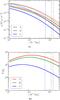 |
Fig. 1 a) Radial density profiles of the gas (solid lines) and DM (dashed lines) of the galaxy cluster models used in this study. The profiles are shown at the beginning of the galaxy interaction, after the cluster models were allowed to relax for ~1 Gyr. Vertical dotted lines indicate the virial radius r200 for clusters A, B, and C, from right to left. b) Corresponding temperature profiles of the ICM. |
2.2. Merger orbits
One of the model galaxies and one of the live galaxy clusters described in the previous section are put on a parabolic merging orbit. The initial conditions for the orbits are set up the same way as in Duc et al. (2000, see Fig. 8 therein for a sketch of the configuration), and, in all of the simulations in this work, the orbital angular momentum is oriented parallel to the z-axis. Instead of using two galaxies, galaxy one in the binary collision set-up of Duc et al. (2000) is replaced with the cluster model, without setting any inclination, hence (Φ1,φ1) = (0,0). The second galaxy is the model galaxy orbiting in the cluster. The different parameters used for the distinct simulations are listed in Table 3. The impact parameter b corresponds to the minimum separation of the cluster and galaxy if they were point masses and moved on Keplerian orbits. Different orbits of the galaxy through the cluster and hence different RP scenarios can be obtained by altering the impact parameter and the initial separation of galaxy and cluster centre.
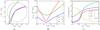 |
Fig. 2 Fiducial galaxy orbits adopted for studying the interaction of galaxy model G1a with the three different galaxy clusters constructed for the study. a) Trajectories of the galaxy in clusters A, B, and C, scaled to the virial radius of the corresponding cluster. b) Time evolution of the distance of the galaxy to the corresponding cluster centre. c) Effective inclination angle of the galaxy (angle between the spin vector of the disk and its instantaneous velocity vector). |
Primary galaxy–cluster interaction simulations performed in this work.
Runs S1 to S4 were carried out with model galaxy G1 in the different clusters, whereas galaxy G2 was used in runs S5 to S7. The angular momentum unit vector of the galactic disk is set to  for runs S1, and S3 - S7, and to
  for run S2. The actual orbits of the different runs are shown in Fig. 2a in units of r200 of the corresponding cluster. Furthermore, the distance of the galaxy to the centre of the cluster and the effective inclination (angle between angular momentum and relative velocity vector of the galaxy) over time is depicted in Figs. 2b and c. All trajectories lie in the xy-plane, and the model galaxies start close to the virial radius of the cluster. Furthermore, in Fig. 3 we show the ICM properties the galaxy encounters while orbiting the cluster by plotting density, relative velocity, corresponding ram pressure, and ICM temperature as a function of time.
The set-up adopted here allows for more realistic scenarios as wind-tunnel experiments. While it is in principle possible to mimic temporal changes of the relative velocity and density of the headwind, varying the inclination angle of the galaxy correctly is difficult. Furthermore, our new set-up also includes a full treatment of gravitational effects from the interaction of the galaxy with the potential of the cluster. This includes tidal truncation of the DM halo as well as tidal effects on the disk itself, which are both not present in ordinary wind-tunnel simulations. These effects not only change the structure of the galaxy, but also influence the conditions under which RPS takes place. On the other hand, the smooth ICM distribution of our live galaxy-cluster models rather resembles a relaxed and virialised system. In future work, we will include dynamically perturbed clusters, especially studying the influence of shock fronts in the ICM on RPS and SFR of cluster galaxies (e.g. Pranger et al. 2014). Also, the investigation and disentanglement of tidal interaction in combination with RPS (e.g. Bischko et al. 2015) in a realistic cluster set-up should be subject of future work.
2.3. Numerical code and star formation model
All simulations presented in this work were performed with the hydrodynamical moving-mesh code AREPO (Springel 2010). Given a set of mesh-generating points, the volume is discretised by a Voronoi tessellation, yielding an unstructured grid. Subsequently, fluxes across each face of a cell are calculated using an unsplit Godunov scheme with an exact Riemann solver in the form of the MUSCL-Hancock finite-volume scheme (van Leer 1984, 2006), which is second order in space and time (for a smooth gas distribution).
As the Voronoi mesh in AREPO is allowed to move with the gas flow and the Riemann problem is solved in the frame of the (moving) face of a cell, it can be shown that the scheme is manifestly Galilean invariant, which is not the case for standard Eulerian codes using static grids. This makes the truncation errors of AREPO independent of the gas velocity. Effectively, the code combines advantages of Eulerian and Lagrangian schemes such as smoothed particle hydrodynamics (SPH) while avoiding some of their disadvantages. In particular, the good treatment of shocks and contact discontinuities of Eulerian schemes is preserved. On the other hand, the scheme inherits the adaptivity and Galilean invariance of SPH. Furthermore, self-gravity is treated as in SPH codes, resulting in a continuous adjustment of the gravitational resolution in a Lagrangian fashion.
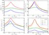 |
Fig. 3 Physical conditions encountered by galaxy G1 as it falls into different galaxy clusters. The top left panel shows the relative velocity of the galaxy, the top right panel shows the ICM density, the bottom left panel gives the resulting ram pressure Pram, and the bottom right panel indicates the ICM temperature encountered by galaxy G1a for runs S1, S3, and S4, respectively. Galaxy inclination does not affect these values significantly, hence run S2 looks essentially the same as S1 and is hence not shown. Also, as in Fig. 2, the values for galaxy G2 in runs S5−S7 are very similar as the trajectories are nearly the same. |
In cosmological simulations, a very high dynamic range in the gas density is present, ranging from ~10-30 g cm-3 in the ICM at the virial radius to well above ~10-22 g cm-3 in the ISM in a galaxy. To avoid numerical artifacts, in SPH an approximately equal mass resolution needs to be used for particles that are in direct contact (Ott & Schnetter 2003; Read et al. 2010), making it difficult to resolve a comparatively small galaxy accurately within a large cluster of galaxies. In AREPO this problem can be much better addressed because there is no restriction on the relative mass content of neighbouring cells, allowing steep gradients in resolution. It is then possible to efficiently simulate a highly resolved galaxy moving around within a poorly resolved background cluster by adaptively refining the region the galaxy passes through.
We use a simple sub-resolution model for radiative cooling, SF, and supernova feedback according to Springel & Hernquist (2003). Radiative cooling is implemented for an optically thin gas of primordial composition (Katz et al. 1996). This gives an effective temperature floor of ~104 K when metal-line cooling is not included. However some gas can cool below this temperature through adiabatic expansion. Star formation and feedback is modelled with a sub-resolution multi-phase description for the ISM on a cell-by-cell basis, since these processes cannot be resolved explicitely. For each gas cell in the star-forming regime (ρ>ρth), the amount of gas is split into cold clouds and a hot, supernova-heated ambient medium. Cold clouds are transformed into stars on a characteristic timescale t⋆, where a mass fraction β is released immediately as supernovae. The released mass as well as evaporated gas from the cold cloud phase replenishes gas in the hot phase again. This leads to self-regulation and, assuming that the temperature of the hot medium evolves towards an equilibrium value governed by cooling and feedback heating from SF, the amount of gas contained in the hot and cold phase can be calculated. This then yields an effective equation of state that stabilises the ISM against too rapid collapse. We note that these processes are modelled separately for each gas cell and no mass exchange or energy release into neighbouring cells takes place. Also, the actual creation of star particles is treated in a stochastic fashion such that the formed collisionless star particles all have roughly the same mass.
We follow Heß & Springel (2012) in choosing the parameters of the sub-resolution model. We set the SF timescale to t⋆ = 1.5 h-1 Gyr. For the supernova feedback model, we use a cloud evaporation parameter of A0 = 104 and a supernova temperature of TSN = 109 K. Furthermore, adopting a Salpeter (1955) IMF, the mass fraction of massive stars (> 8 M⊙) blowing up instantaneously as supernovae is β = 0.1. The choice of those parameters defines the density threshold for the onset of SF ρth = 2.6 h2 cm-3 (see Springel & Hernquist 2003, for a detailed discussion of these parameters). The resulting threshold is higher than that obtained using the default choice of parameters in Springel & Hernquist (2003), which were used e.g. in Steinhauser et al. (2012), Kronberger et al. (2008). This is motivated by recent claims that higher threshold values are needed to obtain more realistic spiral galaxies (Guedes et al. 2011).
Furthermore, we switch on cooling and SF only for the ISM of the galaxy but not for the cluster. To this end, we are using a “colouring” technique (as e.g. Vogelsberger et al. 2012; Roediger & Hensler 2005) to trace the galactic gas throughout the simulation. Each gas cell gets an additional scalar value that is initialised with the gas mass of the cell in case of the cells of the galaxy. This scalar value is then advected with the calculated flux from the hydrodynamic solver. This technique allows us to track the gas of the infalling galaxy in the stripped wake also, in addition to controlling cooling and SF. The latter is only switched on if the galactic gas fraction in a cell exceeds fISM = 0.25. This trick prevents the rest of the cluster from radiatively cooling and forming stars at a high rate in the BCG, which would quickly become numerically very expensive even though we are not interested in the central cluster region itself. We checked that varying this threshold in the range fISM = 0.01−0.25 has almost no impact on the results.
2.4. Refinement technique
As pointed out previously, we need to cover a high dynamic range in density to account for the interaction of the ISM and the ICM. Ordinary grid codes usually use an adaptive mesh refinement (AMR) technique (e.g. O’Shea et al. 2004; Fryxell et al. 2000) to dynamically increase the resolution where needed by creating a hierarchical subgrid in, for example regions with a high density contrast. The resolution can be decreased again by removing levels of the subgrid, for example in regions with a smooth density distribution. Such an approach is also possible in AREPO with its unstructured mesh, although the Lagrangian nature of the code drastically reduces the required number of refinement and derefinement operations when a roughly constant mass resolution (which is often the case) is desired. To this end, single cells can be refined easily by inserting a new mesh-generating point very close to the original one, effectively splitting the cell into two and keeping the rest of the Voronoi mesh unaltered (Springel 2010). The regularity of the mesh is restored in the following timesteps, as the points are moved towards the geometric centre of the corresponding cells. In this work, we use the maximum face angle of a Voronoi cell (Vogelsberger et al. 2012) to decide whether a cell is too distorted and consequently mesh regularisation motions are added to the ordinary movement of the mesh-generating points.
The initial gaseous disks for our model galaxies are generated by distributing gas cells of constant mass according to the desired density profile (see Sect. 2.1). This leads to a higher spatial resolution in the dense, inner parts of the disk and a lower spatial resolution in the outer parts. In our production runs, we are using a gas mass of 7.8 × 10⁴h-1M⊙, corresponding to initially 210 000 gas cells in the disk of galaxy G1 (see also Sect. 4) with a maximum and average spatial resolution of 10 h-1 pc and 160 h-1 pc, respectively. Model galaxy G2 has the same mass resolution and hence fewer gas cells. While the Lagrangian behaviour of the moving mesh adjusts the resolution automatically to the clustering state of matter, we still need a criterion for deciding whether a finer grid in some preferred regions is needed, in our case, for the galaxy and surrounding ICM. For the galactic gas, we want to keep the mass resolution of all cells almost constant at the value in the initial conditions that also defines the target mass for refinement to create star particles of similar mass, which helps to keep two-body heating effects at a minimum level (Vogelsberger et al. 2012).
However, if we impose the same mass resolution for the ICM in the region around the virial radius where the interaction with the galaxy starts, the corresponding ICM cells would have a size comparable to the galaxy itself owing to the low ICM densities there. This can create heavily distorted cells and an underestimation of the gas density in the outskirts of the galaxy.
However, in AREPO, there is no need to have the same mass or spatial resolution for all gas cells, unlike in standard formulations of SPH (Ott & Schnetter 2003). One possible solution to this problem lies in introducing a kind of background grid (Springel 2010), which simply means that there is an imposed upper limit for the maximum volume of cells. In addition, we need to prevent that the denser parts of the ICM that do not interact with the galaxy are all refined to our high target mass resolution, otherwise the computational cost would be completely dominated by following cluster material we are not really interested in.
To address both of these issues, we apply the following three criteria in sequence to decide whether a cell should be refined or derefined: firstly, we use the refinement and derefinement criteria of Vogelsberger et al. (2012) to keep the mass resolution of the ISM close to the initial value for all gas cells with an ISM mass fraction larger than 1%, which we identify using the same colouring technique as described in Sect. 2.3. Such cells are refined or derefined if the mass exceeds two times or is lower than half the target mass of ISM gas cells. Secondly, we require all gas cells to have a volume not larger than ten times the smallest volume of all its neighbouring cells (Pakmor et al. 2013), ensuring a gradual refinement of the ICM around the galaxy and its stripped gas. The third criterion with lowest priority keeps gas cells, which have an ISM mass fraction that is less than 1%, and that are not affected by the maximum volume criterion, at the initial mass resolution of the cluster.
Nevertheless, the volume criterion for refining cells in the surrounding of the galaxy is not necessarily sufficient when the galaxy moves at high speed through the cluster. Because a gas cell can be refined only if it is sufficiently regular (meeting the above-mentioned criterion for its face angles), a certain time is needed until all cells in a region can be transformed to a new (finer) volume. To avoid potential problems from this lag, we refine cells along the a priori known trajectory of the galaxy to the initial mean volume of gas cells in the galaxy itself, so that the ICM gas cells already have a sufficiently small volume and the desired spatial resolution when the galaxy arrives. In the case of our production runs, this initial mean volume corresponds to 52.72 h-3 kpc3 (see also Sect. 4). Also, we make sure that the gradual refinement mentioned above is already realised in the initial conditions. This is achieved by simulating the cluster itself for around 300 h-1 Myr with enabled refinement criteria. Then we insert the galaxy in the relaxed galaxy cluster and start the actual simulation. Tests of the correct functioning of these special refinement techniques and a resolution study can be found in Sect. 4.
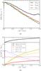 |
Fig. 4 a) Star formation rate of model galaxy G1 when evolved in isolation. The three variants shown correspond to different gas masses in the corona. Model G1a has the same baryonic mass in the halo as in the disk, G1b has half of that mass, and G1c has only 1% of the disk mass in the gaseous halo. b) Evolution of different baryonic components of galaxy model G1a (solid lines) and G1c (dashed lines) evolved in isolation. The red line indicates accreted halo mass onto the disk. The mass components shown are newly formed stars, star-forming (ρ> 2.6 h2 cm-3), and non-star-forming gas. The black line shows the total gas mass in the disk plus newly formed stars. |
3. Results
3.1. Galaxies in isolation
We begin by considering results for our model galaxy G1 when evolved in isolation with different hot halo gas masses. This investigates the evolution of field galaxies depending on the presence of a more or less massive hot gas halo and provides the comparison benchmarks for our simulations with RPS. In Fig. 4a, the evolution of the SFR of the three different galaxies is shown. The model galaxy with the most massive gas halo, which contains the same mass as the disk, shows an enhanced SFR as the disk is refueled by accretion from the hot halo; however, the other two models with only half, or essentially no, baryonic mass in the halo show almost the same SF activity.
In the bottom panel of Fig. 4, we show the evolution of the baryonic mass in the disk with respect to simulation time. We use a simple geometric criterion (a cylinder with r = 20 h-1 kpc and h = 3 h-1 kpc, centred on the galaxy plane) to decide whether gas cells and newly formed stellar particles belong to the disk or the halo of the galaxy and split the gas mass in the disk into star-forming (having a density > 2.6 h2 cm-3) and non-star-forming gas. The amount of low density, non-star-forming gas remains the same in all of the three simulations. Also, the mass of newly formed stars over time is shown while the red line indicates mass that was accreted onto the disk from the hot gas halo during the simulation. The higher mass of newly formed stars due to a higher SFR in the simulations, including a hot gas halo, matches the mass of gas accreted after 2 h-1 Gyr of evolution. We note, however, that our simulations do not include strong feedback processes that could expel significant ISM mass or even unbind hot gas halo (the influence of feedback is discussed e.g. in Nelson et al. 2015). Furthermore, we note that we follow the common assumption that there is no angular momentum transport from the dark matter to the hot gas halo, hence we initialise the hot halo with the same specific angular momentum as the DM halo. Moster et al. (2011) carried out simulations of galaxies in isolation using GADGET-2 (Springel 2005), varying the total angular momentum of the hot gas halo. They found that by assigning the DM halo angular momentum four times to the hot gas halo yields the best results compared to observations of stellar mass and disk scale length. However, also applying the angular momentum four times to our model galaxy G1 does not lead to very different results. Although this lowers the SF slightly, the most important parameter is still the hot halo mass. Presumably, the influence of the angular momentum is also small because our simulations start with a relative high gas mass in the disk with respect to the hot gas halo, compared to the Moster et al. (2011) studies.
3.2. Ram-pressure stripping
Stripping can be broadly subdivided into two classes: ram-pressure pushing (Gunn & Gott 1972), and gas dragging from the outskirts of a disk of a galaxy from Kelvin-Helmholtz instabilities (Nulsen 1982). Ram-pressure pushing can truncate the gas disk of a galaxy out to the so-called stripping radius, where the pressure of the impinging ICM wind  (6)exceeds the gravitational restoring force of the disk,
  (7)Assuming a double exponential profile for gas and stars in the disk, the stripping radius can be calculated as
 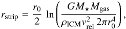 (8)where r0, Mgas and M⋆ is the initial disk scale length, and gas and stellar masses, respectively. The density of the impinging ICM wind is given by ρICM, and vrel denotes the velocity of the galaxy relative to the ICM. As this model is very often used in SAMs (e.g. De Lucia et al. 2004; Guo et al. 2011; Benson 2012), below we test how well it agrees with our simulations. This formulation does not take a possible inclination of the disk with respect to the velocity vector of the galaxy into account.
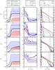 |
Fig. 5 Ram-pressure stripping of galaxy G1a for runs S1−S4 in the corresponding clusters. The panels of the column on the right-hand side show gas surface density profiles of the galaxy (solid lines) and exponential surface density fits based on the gas mass in the galaxy at a particular timestep (dotted lines) as coded by the colours. Vertical dashed lines indicate the radius, at which the actual surface density drops more than one dex below the exponential fit. The panels of the middle column give the evolution of the stripping radius in the simulations, which are determined with three different measurement methods (defined in Sect. 3.2). The blue shaded area encloses the minimum and maximum stripping radius, calculated by different theoretical predictions based on the standard Gunn & Gott (1972) criterion (blue dashed line), considering initial or current and total disk mass, the inclination of the galaxy as well as Rankine-Hugoniot post-shock conditions. The black lines in the panels of the left column show the effective mass lost via stripping in the simulations. The edges of the blue shaded region indicate the minimum and maximum mass loss, considering the stripping radius calculated with the different models. The red shaded area depicts the corresponding extrema of mass loss due to a continuous stripping assumption. The yellow dashed lines indicate the model that best fits the corresponding simulation. |
In previous work, it has been found that the above relation is quite accurate for face-on galaxies (e.g. Kronberger et al. 2008; Roediger & Brüggen 2007), and that the inclination angle does not seem to have a large impact on the amount of stripped gas as long as the inclination is not close to edge-on (e.g. Steinhauser et al. 2012; Jáchym et al. 2009; Roediger & Brüggen 2006). Nevertheless, there are modified theoretical descriptions that take the inclination of the galaxy into account (e.g. Lanzoni et al. 2005) by adding a  factor to the RP term. Other variations consider the total mass of the galactic disk when calculating its potential, hence computing a more accurate estimate of the restoring force (e.g. Font et al. 2008).
Also, the above model is intended for a single stripping event at constant RP, and assumes that the surface density profile of the disk within the stripping radius is not altered after the stripping event. However, in reality, RPS is not an instantaneous process with the stripping radius and hence the amount of stripped gas settling down only after ~10−100 Myr in typical wind-tunnel experiments. Furthermore, during cluster or subhalo infall, the density and velocity change continuously. Also, galaxies can move at a higher velocity than the local sound speed, leading to the formation of a bow shock in the ICM that is impacted. Calculating the velocity and density of the ICM behind the bow shock with the Rankine-Hugoniot conditions (Shu 1992), one finds that the RP behind the bow shock is less effective than the classical approach suggests when the shock is ignored.
In the following, we hence compare the stripping radius and gas loss in our simulations with all possible combinations of the aforementioned variations of the original Gunn & Gott (1972) criterion, using ρICM and  and also the total remaining gas and stellar mass of the galaxy from every snapshot of the simulations. We calculate the gas loss due to Kelvin-Helmholtz instabilities, which are also referred to as continuous stripping, following Nulsen (1982) and Roediger & Brüggen (2007), as
 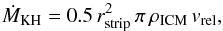 (9)using the calculated theoretical stripping radius for all distinct variations.
In Figs. 5 and 6 we show the results for galaxies G1a and G2 respectively, for different environments. In the column on the right-hand side, the surface density profiles of the galaxy (solid lines) are shown after 0, 400, 800, 1200, and 1600 h-1 Myr of evolution in the corresponding cluster; this is compared to the theoretical, exponential density profile the galaxy would have when the scale radius is kept constant at the initial value and the normalisation is updated to the remaining gas mass in the disk at a particular timestep, as coded by the colours (dotted lines). The vertical dashed lines indicate the radius, where the surface density of the galaxy falls more than one dex below the theoretical, exponential profile mentioned above. This is useful for calculating the stripping radius, as described in the next paragraph, and also allows us to investigate a possible redistribution of gas to the outer parts of the disk.
In the middle column, the stripping radius versus simulation time is shown. Determining the exact radius in an automated way is not a trivial task; even investigating every snapshot visually often does not lead to clearly defined radii. Therefore, we plot three different stripping radii assigned with different methods. In the first case (blue solid line), we determine the stripping radius at the point where the actual surface density profile in the simulation drops more than one dex below an exponential surface density profile (3), using the remaining gas mass in the disk of a particular timestep and the initial disk scale length (see previous paragraph and compare the dotted to the solid lines at different timesteps in the panel on the right-hand side). Secondly, following the approach by Roediger & Brüggen (2006), we divide the disk into 12 segments and determine the radius for each. As the mass in the cells should be equal and close to the target mass of the ISM gas (see Sect. 2.4), we divide the segments into radial bins and define the stripping radius as the bin with less than ten gas cells. Then, the red line indicates the stripping radius as the mean value of all segments. This approach has been found to yield the most robust measure for all simulations performed in this work. Finally, we also consider the still gravitationally bound gas mass, considering also gas transformed into stars. For each snapshot we calculate the radius that the galaxy would have if the initial surface density profile were not altered (green line). As can be seen in the plots, this method does not consider the delay between the gas that is pushed out of the disk and the gas that is not gravitationally bound to the galaxy anymore. However, considering this lag, and in cases of constant RP (as in cluster B), it is a reasonably good measure and agrees well with the other methods. Finally, we sketch the results of theoretical predictions described at the beginning of this section, comprising the standard Gunn & Gott (1972) criterion and variations including the total mass and inclination angle of the disk as well as considering Rankine-Hugoniot post-shock conditions. The blue dashed line indicates the stripping radius calculated with the standard criterion (8). The blue shaded area delimits the range of stripping radii from all theoretical predictions mentioned above, with the edges corresponding to minimum and maximum values at any time.
In the column on the left-hand side, the actual gas mass stripped from the disk is plotted (black solid line). We consider that all gas not bound gravitationally to the galaxy anymore (gas cells that have a positive total energy Etot = Epot + Etherm + Ekin) are stripped off the disk. Usually, gas is being pushed out of the disk and stays gravitationally bound until the gas is sufficiently decelerated. To calculate the stripping radius and the surface density profile, we therefore only consider the gas in a cylinder around the galaxy. We note that gas is lost also due to SF. Furthermore, we calculate the mass loss considering the theoretical predictions of the stripping radius from the different models mentioned above. Again, the edges of the blue shaded area depict the minimum and maximum of the mass loss calculated from different models. The blue dashed line once more indicates the mass loss using the standard Gunn & Gott (1972) criterion. The red shaded area delimits minimum and maximum mass loss due to continuous stripping, using the stripping radius from the different models, denoted above in Eq. (9) and applying the current RP at any time. The yellow dashed line depicts the best model for the corresponding simulation, which is described later in this section.
The results in Fig. 5 show different behaviour for the RPS of a Milky-Way sized galaxy G1a in different environments. The first extreme case of RPS in cluster A (see also Sect. 2.1) strips the gas disk of the galaxy almost completely during pericentre passage, as expected. Considering also the SF activity, only 12% of the gas is left in the very centre of the disk. Similarly, when the galaxy starts with a different inclination angle (run S2), around 15% of the gas is left after pericentre passage. This indicates that the inclination does not have a major influence on the total amount of stripped gas. However, the inclination of the galaxy in both runs differs most at the beginning of the simulation when RP is still low (face-on vs. edge-on), whereas at the peak of RP the inclination becomes quite similar (see Fig. 2c). Furthermore, the stripping radius for both inclinations is also similar, dropping from 18 h-1 kpc to around 1−2 h-1 kpc after 600 h-1 Myr. Ram-pressure pushing lasts until the galaxy reaches the peak of RP at pericentre passage. Afterwards, continuous stripping proceeds at a very low rate as a result of the small remaining gas disk, which is depleted by forming new stars.
In the smaller cluster B, the trajectory was chosen to have a slowly changing, medium RP acting on the galaxy (see Fig. 3). As a consequence, the galaxy keeps losing gas throughout the whole simulation mainly by continuous stripping, but at a much smaller rate than in cluster A. In cluster/group C on the other hand, the trajectory again leads more towards the centre and has an overall less pronounced RP but a higher peak at pericentre passage. In this case, gas is lost mainly from 400−700 h-1 Myr when the galaxy experiences high RP. At the same time the stripping radius is reduced to 10 h-1 kpc. Before and afterwards, the galaxy is mainly affected by continuous stripping, which proceeds however at a very low rate of < 1 M⊙ yr-1.
In simulations with a high peak of RP (S1, S2 and S4), the radius of the gas disk is again increasing when the galaxy leaves the central region of a cluster (red and blue lines in the middle column of Fig. 5). The strength of the effect however depends on the method used for determining the radius (see description above for the different methods used). Using a fixed cut (red line), the effect is small, showing a maximum expansion of 2 h-1 kpc in run S4. However, comparing the actual surface density with an exponential profile, considering initial disk scale length and remaining gas mass in the particular timestep, shows an increase of up to 5 h-1 kpc. Hence, the strong increase, seen in this case, is mainly due to a shallower exponential profile the actual surface density of the galaxy is compared to. Furthermore, in such cases, the surface density can be described well with the mentioned exponential profile at radii sufficiently below the stripping radius. It is as if an “overcompressed” disk expands slightly again.
Very similar results are found for model galaxy G2 and are presented in Fig. 6. This smaller galaxy gets stripped completely when passing the central region of cluster A. Passing through clusters B and C, the stripping radius drops from the initial 15 to 6 and 4−5 h-1 kpc, respectively. Similar to galaxy G1, in cluster C the redistribution of the gas in the disk can be observed after pericentre passage when the strength of RP is decreasing again. However, the effect is limited to the outer parts of the disk. The surface density at smaller radii, not affected by RPS, shows no change compared to the initial profile.
The stripping radii calculated with theoretical RPS models described above can differ by as much as 5 h-1 kpc with corresponding consequences for the estimated gas mass that is stripped as well, especially when it comes to the inner parts of the disk. The best model fitting our simulations depends on environment, but also on the mass of the galaxy itself. For the more massive galaxy, G1, the theoretical model, which takes into account the appearance of supersonic velocities and the current gas and stellar mass in every snapshot, yields results closest to runs S2 and S3, if one also considers the mass lost after pericentre passage from continuous stripping in the simulations. With different initial inclination of the galaxy (run S1), the standard model and when RP is scaled with the effective inclination of the galaxy also provides reasonable results. In run S4, with a high peak of RP, using the initial disk mass gives the best results. For galaxy G2, the model that best fits all simulations includes Rankine-Hugoniot post-shock conditions and uses the initial disk mass, hence assumes a constant surface density profile to calculate the stripping radius. However, in all of the cases and for both model galaxies, considering the total mass in the disk yields much better results than the standard criterion. All of the mentioned models are depicted in the panels on the right-hand side in Figs. 5 and 6 as yellow dashed lines. Furthermore, SF needs to be taken into account, as a sizable fraction of gas in the disk is transformed into stars on the timescale of one cluster centre passage (see also Sect. 3.5).
In Fig. 7, we show 100 × 40 h-1 kpc slices in the yz-plane that are centred on the disk of the galaxy of run S1 at time 600 h-1 Myr (just at pericentre passage), which are produced using adaptive kernel smoothing by first computing SPH-like smoothing lengths for the mesh-generating points and then distributing the corresponding quantity onto a regular grid using the SPH kernel. Although in the chosen snapshot the highest RP of all simulations acts on the galaxy, losing mass at the highest rate, gas is still diluted and heated fast as soon it is stripped. Around 50 h-1 kpc behind the disk, most of the gas has heated up and is already diluted to the background density of the ICM. On the other hand, mixing with the ICM proceeds at a slower rate as can be seen in the lower panel: the metallicity shows a slower decline in the stripped wake.
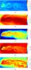 |
Fig. 7 Slices of thickness 0.2 h-1 kpc and extension 100 h-1 kpc × 40 h-1 kpc through the galaxy and its wake in run S1, after 600 h-1Myr of evolution. Quantities are mapped using an SPH kernel. The different panels show: a) gas density, b) velocity magnitude, c) metallicity, d) temperature, and e) vorticity magnitude. |
The stripping of the hot gas halo proceeds very fast in all of the simulations. After 50−150 h-1 Myr, 80−90% of the gas mass in the hot halo is being stripped. Only a small fraction that either resides very close to the galaxy or is in the slipstream of the disk stays bound to the galaxy. In SAMs (e.g. Guo et al. 2011), stripping of the hot gas halo is very often modelled with two processes: by either assuming full stripping at a radius where the RP exceeds the gas pressure of the halo or by invoking tidal stripping in which the gas mass is reduced from the hot halo in direct proportion to the DM halo mass during infall. Looking at our simulations, only the first process comes into play, as the stripping advances quickly, already in the outskirts of the cluster, whereas the DM halo loses mass significantly only after pericentre passage. We also note that McCarthy et al. (2008) have shown that the truncation radius due to tidal stripping is only smaller compared to the RPS radius if the galaxy exceeds 10% of the cluster mass, which is not the case in any of our simulations.
3.2.1. Metal enrichment
Ram-pressure stripping is an important process (Domainko et al. 2006) contributing to the metal enrichment of the ICM in galaxy clusters (e.g. Schindler et al. 2005; Schindler 2007; Werner et al. 2008; Zhang et al. 2011). Here, we investigate the enrichment of the ICM by means of RPS from a single galaxy. The treatment of SF we use (Springel & Hernquist 2003) tracks only the total metal mass and assumes solar composition. This is done by means of a scalar value that is advected with the calculated mass flux derived from the hydrodynamic solver, which is similar to the colouring technique employed in the refinement. The metal yield is set to p = 0.0122 (Asplund et al. 2005) and is used throughout all of the simulations.
As we start our simulations with a gas fraction of 35% in the disk, the initial metal content is important for the metal enrichment of the ICM due to RPS. Observations show a huge diversity in radial metallicity profiles of disk galaxies (e.g. Zaritsky et al. 1994; Bresolin et al. 2012). However, as in Höller et al. (2014), we decided to model the metallicity gradient in our model galaxies using mean values of observations from Ferguson et al. (1998),  (10)approximating R25 ≃ 3.5r0, and using solar values from Asplund et al. (2005) again to translate from oxygen abundance to total metallicity values. The total metal mass in the gas disk is given by the mass of the old stellar disk, according to the model presented in Sect. 3.4.
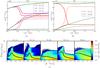 |
Fig. 8 Panels a) and b): evolution of metal mass in both model galaxies as a function of simulation time for interactions with clusters A or B, respectively. The solid lines indicate the metal mass in both gas and newly formed stars that are gravitationally bound to the galaxy, whereas the dashed lines give the metal mass locked up only in newly formed stars. The dotted lines indicate the metal mass in the stripped gas wake. Panel c): metallicity histograms of stripped gas (considering gas cells not gravitationally bound to the galaxy anymore and with ISM mass fraction >1%) as a function of time. The colour encodes the mass fraction in each metallicity bin of the total gas mass stripped for each timestep. The black solid line shows the mean metallicity value of the gas cells in the histogram, while the dashed line indicates Z⊙. |
 |
Fig. 9 a), b) Evolution of the |

In Figs. 8a and b, we plot the total mass of metals in gas and stars still gravitationally bound to the galaxy (solid lines) and metals locked up in newly formed stars (dashed lines). Furthermore, the metal mass in stripped gas (dotted lines) for galaxies G1a and G2 is depicted, respectively. Here we do not include the metals in the old stellar disk, as the mass there does not change throughout the simulation and no stars are stripped. As expected, as SF is quenched after pericentre passage in cluster A in both galaxies, fewer metals are present in total than in cluster B, although the effect is very small. The more massive galaxy can enrich the ICM with around 2 × 10⁸h-1M⊙, which is almost half of its initial metal content in the ISM. The smaller galaxy loses 0.8 × 10⁸h-1M⊙, which accounts for about 80% of its initial metal mass. In cluster B, where only weak but continuous stripping takes place, only a few metals (< 5% for G1a, < 20% for G2) are transported to the ICM because only the outer parts of the galaxy with a lower metallicity are stripped. Hence, with respect to their gas mass and metal content in the disk, the smaller galaxy G2 is enriching the ICM with a relative higher amount of metals. We note that the gas of G2 is more easily stripped because of the shallower gravitational potential when the same RP is exerted.
The inclination of the galaxy has an effect on the metal enrichment of the ICM and the amount of stripped gas. The purple line corresponds to run S2 with the galaxy starting edge-on. During pericentre passage, more metals are locked up in newly formed stars, as SF is enhanced with respect to run S1 (see Sect. 3.3). In total, less gas is stripped in S2 with respect to S1 (see Sect. 3.2), which translates to a relatively smaller amount of metals transported to the ICM.
The differences however are more evident in Fig. 8c. We plot the metallicity Z of stripped gas in a histogram ranging from 0.15 Z⊙ (our initial value adopted for ICM gas) to 5 Z⊙ for each snapshot throughout the simulation. Thereby, we consider all gas cells with at least 1% of its mass originating in the galaxy itself. The colour encodes the mass fraction of stripped material in different metallicity bins. The black solid line indicates the mean metallicity of the gas considered in the histogram. In cluster A, the mean metallicity in stripped material for both simulations with the galaxy starting edge-on and face-on are not very different, reaching a peak of almost Z⊙ at pericentre passage. Afterwards, when no gas is stripped anymore and owing to the mixing with the ICM, the mean metallicity decreases again. However, more metal-rich gas from the centre of the galaxy is stripped edge-on in the first 500 h-1 Myr of the simulation, which is diluted quickly afterwards. Stripping is going on for the larger galaxy until the end of the simulations. In both cases, progressively more of the enriched material from the centre is stripped, but the total amount nevertheless stays small. The stripped material of the smaller galaxy on the other hand has a higher metallicity right from the beginning, as the metal-rich inner parts of the disk are stripped earlier. However, mixing of ISM and ICM in the wake proceeds in the same way for both galaxies (runs S1, S2, and S5, respectively), hence considering that they have a similar ISM metallicity their mean metallicities in the wake also end up the same at the end of the simulations when all the gas has been stripped.
In cluster B, with a slow but continuous stripping rate, the gas wake of the smaller galaxy has a higher metallicity again, reaching up to 1.6 Z⊙ with the mean value reaching as high as 0.6 Z⊙. For both galaxies, the supply of stripped, enriched material balances mixing with the ICM. Mixing and hence a drop of the metallicity can also be seen in Fig. 7c, where a slice of the metallicity in the stripped wake of run S1 after 600 h-1Myr is shown. The metallicity of stripped gas right behind the galaxy drops by a factor of 2−3 already after around 100 h-1 kpc behind the disk while the gas is mixed with the ICM.
3.3. Star formation
In the following section, we investigate the SFR in the simulations with a focus on the dependence of galaxy mass and environment on quenching.
As the hot gas halo of the more massive galaxy G1a is stripped right at the beginning of the simulation, in the first 500 h-1 Myr, the SFR in all of the clusters drops to the values of the isolated galaxy without hot gas halo (G1c); this is also because in this phase, not much gas in the disk is lost due to RP (see Fig. 9c). In cluster B, the SFR of the galaxy follows the same profile as G1c in isolation throughout the whole simulation. The weak RP in this case, which only leads to continuous stripping in the outskirts, does not affect the SFR significantly. In contrast, in cluster C, at the short but high peak of RP, the SFR is enhanced by at most 2 M⊙ yr-1 as the disk gets compressed. Afterwards, the SFR only slowly declines and finally drops below the SFR in isolation from a lack of gas in the disk. A similar scenario happens in cluster A: first SFR is enhanced and then drops below isolation levels after big parts of the gas disk are stripped and finally depleted by residual SF. However, this process proceeds much faster than in cluster C, since a higher amount of gas is stripped during pericentre passage because of the stronger RP. In run S1, only a slight enhancement of the SFR to isolation levels (G1a) can be observed. As a result of a different inclination and consequently delayed gas stripping in run S2, more gas remains in the galaxy at pericentre passage when the gas disk is being compressed most. In that case, the SFR can be enhanced by up to 3 M⊙ yr-1, but drops in the same way afterwards. However, almost 109h-1M⊙ more stellar mass can be formed in total by the end of the simulation. In cluster C, the cumulative amount of new stars is largest, and very similar to the amount formed in isolation.
The less massive galaxy G2 shows basically the same behaviour as G1 in the distinct cluster environments (see Fig. 9d). In cluster B, similar to galaxy G1, SFR is slightly enhanced compared to simulations of the respective galaxy in isolation, including the least massive hot gas halo (G1c and G2, see Table 1). In cluster A, again an initial enhancement of the SFR can be observed before most parts of the gas disk are stripped. However, the momentary enhancement of around 20% is smaller than for galaxy G1, which shows an increase of 30−60%, depending on the initial inclination of the galaxy. Finally, the biggest difference between the two model galaxies can be found in cluster C. Despite the similar enhancement of the SFR at pericentre passage, compared to G1 the SFR of G2 is higher than in isolation until the end of the simulation, although relatively more gas is stripped in G2.
The specific SFR ( ) is shown in Figs. 9a and b. The value of the main sequence of SF and 0.3 dex scatter for the particular stellar mass of both model galaxies, taken from Schawinski et al. (2014), are represented with the horizontal black solid and dashed lines, respectively. The grey shaded area below the main sequence indicates the region where “green-valley” galaxies, a transition population between star-forming and passively evolving quenched galaxies, can be found. The more massive galaxy starts its evolution 0.3 dex above the main sequence of Schawinski et al. (2014). Throughout the simulation in isolation and in cluster B, the galaxy stays within the 0.3 dex scatter around the main sequence. In cluster C, the galaxy only falls below the main sequence at the end of the simulation. In the case of extreme RP (cluster A), the galaxy leaves the main sequence only after 1 h-1 Gyr of simulated time, a few hundred h-1 Myr after pericentre passage when the peak of RP is experienced. The difference in run S2 for a different inclination of the galaxy is again small, except for the more pronounced enhancement after around 600 h-1 Myr. Afterwards, the galaxy still needs half of the simulation time to pass through the green valley region in both runs S1 and S2. The smaller galaxy also stays on the main sequence of SF in all environments, except in cluster A. As the SFR suddenly drops to zero when all the gas is stripped during pericentre passage, the galaxy leaves the main sequence quickly and passes through the green valley in less than a hundred h-1 Myr.
In summary, a weak, continuous RP (B) removes the gas supply from the hot halo but does not further influence the SFR. On the other hand, a strong, short RP event (C) , although removing double the gas mass from the disk through stripping, can compress the disk in such a way that the SFR is enhanced such that the same amount of stars is formed by the end of the simulation as in the isolated case. A galaxy can lose all of its gas and drastically quench its SF only in extreme cases of RPS (A). As expected, as less massive galaxies are more prone to lose their gas due to RPS, they are also quenched more rapidly.
3.4. Colour evolution
In this section, we study the colour evolution of the model galaxies evolving in isolation and undergoing RPS. We are particularly interested in how fast a galaxy becomes red when infalling to a galaxy cluster. Furthermore, studying the colour evolution of the galaxy, we can compare with observations and investigate the morphology by generating mock colour images.
As the stellar particles of our model galaxies have masses in the range of ~104−105M⊙, they can be considered simple stellar populations (SSP, e.g. Querejeta et al. 2015; Murante et al. 2015). We are using the flexible stellar population synthesis code FSPS (Conroy et al. 2009; Conroy & Gunn 2010) to calculate SSPs out of the stellar particles of the simulation. The output of FSPS includes observed mock spectra of an SSP given its metallicity and age. By convolving with a desired filter function, the luminosity and hence magnitude of the SSP in the desired band can be obtained. In this work, we use the SDSS bands u, g, r, i, and z as well as Buser B, U, V, and IR K filters. We then calculate the colour for a stellar particle (SSP) via a 2D interpolation of the FSPS tables for different stellar age and metallicity.
Newly formed stars generated during the simulation inherit the metallicity of the gas cell they were formed of. Also, the age of the SSP for those particles is known as the time of generation is stored. For such particles, colour calculation is straightforward, but it is more difficult for the old stellar disk and old bulge particles (types 2 and 3) already present in the initial conditions (see Sect. 2.1) because they do not contain age and metallicity information. Therefore, for our model galaxies we assume a τ-model for SF prior to the start of the actual simulations. We use Eq. (1) of Feldmann & Mayer (2015) to calculate the SF history of our model galaxy, ![\begin{equation} \mathit{SFR}(t) = \mathit{SFR}(t_\star)\left[ (1-c) \exp\left(\frac{t-t_\star}{\tau}\right) + c \right], \end{equation}](/articles/aa/full_html/2016/07/aa27705-15/aa27705-15-eq178.png) (11)and assign age and metallicity to the old stellar disk and bulge particles. In this model, the SFR of the galaxy peaks at time t⋆. For our model galaxies this occurs at the beginning or shortly after the start of the simulation. The value τ is the SF timescale. The value of τ is positive for an exponentially growing SFR, which we assume to be the case for our model galaxies for times prior to the start of the simulation. Hence, SFR(t⋆) is the peak SFR, which we get directly from our simulations. The constant c is an offset for the exponential growth or decline of the SFR, modelling different phases of galaxy formation like gas accretion or starvation phase (for more details see Feldmann & Mayer 2015). We neglect these different phases of galaxy formation and calculate the parameters of this model for our simulated galaxies in the following way. Given the mass of the old stellar disk and bulge, the integral of the SF history is set. Assuming that the overall age of our model galaxies at the beginning of our simulations is 7 Gyr and given the peak star formation rate
(11)and assign age and metallicity to the old stellar disk and bulge particles. In this model, the SFR of the galaxy peaks at time t⋆. For our model galaxies this occurs at the beginning or shortly after the start of the simulation. The value τ is the SF timescale. The value of τ is positive for an exponentially growing SFR, which we assume to be the case for our model galaxies for times prior to the start of the simulation. Hence, SFR(t⋆) is the peak SFR, which we get directly from our simulations. The constant c is an offset for the exponential growth or decline of the SFR, modelling different phases of galaxy formation like gas accretion or starvation phase (for more details see Feldmann & Mayer 2015). We neglect these different phases of galaxy formation and calculate the parameters of this model for our simulated galaxies in the following way. Given the mass of the old stellar disk and bulge, the integral of the SF history is set. Assuming that the overall age of our model galaxies at the beginning of our simulations is 7 Gyr and given the peak star formation rate  from the simulation, all parameters can be set. We use c = 0 for all of our model galaxies. The stellar mass produced in each time bin can be calculated by dividing the 7 Gyr of galaxy formation into time bins given the SFR by the above described model. Randomly, a number of stellar particles are selected, first from the bulge (which is usually considered older than the disk, e.g. Athanassoula 2005) and then from the old stellar disk according to the mass in the time bin. The time of this bin is then assigned to those particles. To compute metallicities for those particles (see also Sect. 3.2.1), we proceed as in Springel & Hernquist (2003). Given the produced stellar mass, the metallicity of surrounding ISM can be calculated immediately for each time bin. The metallicity obtained in this way is assigned to the stellar particles the same way as their age. Values for age and metallicity for the old stellar and bulge particles are assigned once and used to calculate galaxy colours for all snapshots of the simulation to correctly model morphological evolution of the galaxy.
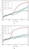 |
Fig. 10 Colour evolution (in the u-i index of the SDSS) of galaxies G1 (top panel) and G2 (bottom panel) as a function of time while interacting with different cluster environments. The slow evolution towards redder colours in the interactions with clusters B and C is actually very similar to the evolution of the galaxies in isolation, showing that the gas consumption timescale is not significantly affected by RPS in these models. This is different in the deep interaction with cluster A, where a rapid shutdown of SF is achieved. |
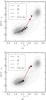 |
Fig. 11 Colour–colour diagrams showing the evolution of galaxies in NUV-u vs. u-r space as they interact with different clusters. The top panel is for model galaxy G1, and the bottom panel for G2. The colour is indicating different environments as shown in the legend. Stars mark simulation times with their brightness encoding 0, 0.5, 1.5 and 2 h-1 Gyr (the brightness corresponds to the one used for the big squares in Figs. 9a and b). The grey shaded contours represent the densities of the observed early- (upper right concentration) and late-type (lower left peak) galaxy populations, as determined by Schawinski et al. (2014). |
In Fig. 10 we present the SDSS u - i colour evolution of our different runs. The values agree well with SDSS data from Weinmann et al. (2010) for both of our model galaxies. In isolation, both galaxies have practically the same colour. Also in clusters B and C, the colour is very similar to the isolated case, although the SFR is quite different, tending slowly towards a redder colour. As soon as SF is quenched, the colour turns red quite quickly in cluster A alone; this is the case especially for the less massive galaxy on timescales of a few hundred Myr. Afterwards, reddening proceeds again at a smaller pace, comparable to galaxies that still form stars.
When SF is quenched, immediate differences can be seen at short wavelengths. Therefore, in Fig. 11, we show a colour–colour diagram considering NUV-u versus u - r colours according to Schawinski et al. (2014). By investigating the different paths of the model galaxies, one can infer quenching timescales as well. The grey shaded contours in these plots indicate the early- and late-type galaxy populations that we reproduced from Schawinski et al. (2014). The colour of the lines corresponds to different paths for the distinct simulations with the shading indicating simulation time as in Figs. 9a and b. Every 500 h-1 Myr is indicated by a star for galaxies in a cluster environment and by a circle for galaxies in isolation. In all of the scenarios, except for the extreme RP case, the model galaxies stay within the late-type population. The path for both galaxies connects to the early-type population in cluster A alone. Whilst the more massive galaxy needs almost a h-1 Gyr to pass the region between the two galaxy populations, referred to as green valley, the transition for the smaller galaxy is much faster, taking a few hundred h-1 Myr, because SF is quenched immediately.
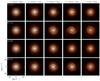 |
Fig. 12 Mock colour images of galaxy G1a in different environments. The evolution in isolation and runs S1, S3 and S4 are depicted in the different rows. In each column, the state at a selected time (indicated on top) is shown for each simulation. |
Finally, we produce spatially resolved mock observations of the model galaxies such as those in Lupton et al. (2004), however, we use a logarithmic stretch for the colours and mapping IR K to red, Buser B to green, and Buser U to the blue image channel following Marinacci et al. (2014). First, to generate an image, particle colours need to be mapped to a grid. To this extent, we use the same approach as for Fig. 7, distributing colour information of the particles with an SPH kernel to a regular grid. Afterwards, a projection of the different bands is mapped to RGB image channels to generate a 2D image. The evolution of galaxy G1a in isolation and the three model clusters (runs S2, S3, and S4) is shown in Fig. 12, respectively. Clearly, in isolation, the spiral structure of the galaxy is retained throughout the whole simulation. Also, more blue light is coming from the spiral arms where SF is also going on at the end of the simulation. The morphology of the galaxy is almost the same in cluster A for the first ~500 h-1 Myr. At pericentre passage, morphology gets distorted as a result of tidal interaction with the gravitational potential of the galaxy cluster. In both cases, a bar in the centre of the galaxy is visible and, apparently, in the cluster the spiral structure is lost. With moderate RP in run S3, the spiral structure is retained the same way as in the isolated case. However, the galaxy is redder in the last snapshot presented at t = 1.6 h-1 Gyr, as the SFR drops below the isolated case. On the other hand, in run S4, morphology gets distorted, especially in the outer parts, showing the typical patterns of tidal interaction, although the overall colour of the galaxy is the same as in run S3.
3.5. Comparison to semi-analytic models
In Sect. 3.2 we have seen that in all of the scenarios the hot gas halo is stripped almost instantaneously when RP sets in. Hence, although there are different implementations for stripping the hot gas halo (see also Sect. 3.2) in SAMs, we only consider stripping of the gasesous disk of galaxies. To this intent, using the parameters of model galaxy G1c without hot gas halo, we implement the standard stripping model for the disk, according to Gunn & Gott (1972). Besides gas stripping, we include SF (Cora 2006; Lagos et al. 2008) but no models for AGN feedback. In order to determine the colour evolution, assuming instantaneous recycling approximation (e.g. Benson 2012), we calculate the metal evolution according to Springel & Hernquist (2003). In each timestep, we assume that a SSP is being formed, calculating its mass from the current SFR and assigning current gas metallicity. An initial evolution of the stellar population of the galaxy is carried out as described in Sect. 3.4.
In Fig. 13, we compare the SFR (a) and colour evolution (b) of our simulations of model galaxy G1 in three different environments (runs S1, S3 and S4) with the evolution of the corresponding galaxy in a SAM, as described above. Thus, extracting the ICM properties along the orbit of the respective simulation, we calculate the theoretical stripping radius and stripped gas mass according to Eq. (8) in Sect. 3.2. Then, the SFR is calculated according to Eq. (3) in Cora (2006), 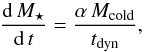 (12)where cold gas mass is Mcold and the dynamical time of the galaxy is tdyn. For the dimensionless parameter
 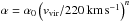 , we chose α0 = 0.18 and n = 2.2 such that the SFR and total stellar mass produced after 2 h-1 Gyr in isolation resemble values of model galaxy G1c. Initially, for the cold gas mass Mcold, we use the mass in the star-forming regime of model galaxy G1c.
Adopting the prescription for SFR of a SAM (Eq. (12)) combined with the RPS model (Eq. (8)) as described above, leads to the following results. Since the SFR is directly related to the available cold gas mass Mcold in the disk, in cluster A the SFR drops below 1 M⊙ yr-1 at pericentre when the stripping radius attains its minimum. The same behaviour can be observed in cluster C. After pericentre passage, the remaining gas is consumed as new stars are formed, since a growing theoretical stripping radius does not provoke further stripping nor is the disk refueled by gas. In cluster B, the weak RP leads to a slow but constant mass loss that leads, however, to a lower SFR than in isolation. Comparing those results with our simulations, mainly two differences are evident. First, even a weak RP can enhance the SFR in the disk, leading to a higher SFR in cluster B than in isolation, which is not reproduced by the SAM, where the SFR is actually lower in the cluster environment. The difference is even more striking in cluster A and C. As a consequence, the simulation produces almost double the amount of stars in cluster A and C at the end of the 2 h-1 Gyr of evolution than the SAM. In cluster B, the stellar mass only differs by 26%, however. Furthermore, as RPS takes some time to strip the gas from the galaxy (see Sect. 3.2), SFR also does not drop immediately as it is the case in SAMs. So although the drop of the SFR in cluster A is very similar as in the simulation, it is delayed by a few hundred Myr. Despite those differences, at the end of the simulation the SFRs agree well in all of the cases.
The corresponding colour evolution is shown in Fig. 13b. Obviously, the differences are largest when the current SFR of simulations and SAM differ most at pericentre passage. The trend of higher SFR in the simulations compared to the SAM expectation is again reflected in the u - i colour as simulated galaxies are generally bluer. However, at the end of the simulation, again the colours coincide well between simulation and SAM, except in cluster A, where the simulated galaxy is much redder than expected from the low level of SF predicted by the SAM.
4. Resolution tests
Given the large dynamic range in density that needs to be covered, it is important to examine how robust our results are when the numerical resolution is changed. The initial conditions of Springel et al. (2005) for the model galaxy evolving in isolation and in combination with our SF recipe have already been subjected to a resolution study as well as a comparison between AREPO, VPH (Heß & Springel 2010), and SPH (GADGET-2) in Heß & Springel (2012). These studies found that the SFR grows slightly with increasing resolution, but tends to converge at high resolution. Simplified wind-tunnel (Heß & Springel 2012) and cosmological simulations (Vogelsberger et al. 2012) show that gas stripping is more efficient in AREPO than in SPH. Furthermore, stripping becomes less efficient with increasing resolution in AREPO.
Mixing and fluid instabilities (especially Kelvin-Helmholtz instabilities) are important processes in RPS simulations. Springel (2010) showed that comparatively such fluid instabilities are modelled accurately in AREPO thanks to its Galilean-invariance even for large bulk flows, which is the case for galaxies falling into a galaxy cluster. Also, overmixing due to advection errors in bulk flows should be reduced. Yet, limited numerical resolution can qualitatively change the outcome of simulations that are sensitive to the development of fluid instabilities, hence we carry out a numerical resolution study of our RPS simulations to quantify the uncertainty related to this.
For our resolution study, we use the trajectory and model cluster A of our fiducial case, run S1 (see Table 3 in Sect. 2.2). This rather extreme case fits best to test our simulation set-up because the galaxy experiences a very high relative velocity and encounters high ICM densities on its way through the cluster, which is best suited to test the proper functioning of the refinement of the ICM gas surrounding the galaxy.
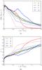 |
Fig. 13 Comparison of the simulations with SAM expectations. a) The SFR of galaxy G1a in cluster A, B, and C (runs S1, S3, and S4, respectively) and galaxy G1c is depicted with solid lines. The dashed lines correspond to the SFR of galaxy G1c with standard prescriptions for RPS (Gunn & Gott 1972) and SF (Cora 2006). In b), the same comparison is shown for the time evolution of the galaxy colours. |
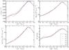 |
Fig. 14 Convergence study of the time evolution of the ICM properties measured in the surrounding and 45 h-1 kpc in front of the galaxy. |
Different runs carried out for the resolution study.
In our resolution study, we carry out simulations of the same model with different resolutions for both ISM and ICM as well as different refinement approaches. The different runs are listed in Table 4. First, as we are mainly interested in the evolution of the model galaxy, we change its mass resolution by factors of ten and adapt the resolution of the refined ICM in front of the galaxy accordingly. The corresponding target volume of ICM gas cells is given in Table 4 as well. The target volume is only valid for gas cells in the ’tunnel’ along the trajectory of the galaxy through the cluster and is defined as the mean volume of the gas cells within the model galaxy. As a result of the gradual refinement around ISM gas cells, the resolution of ICM gas cells interacting with the galaxy is defined by the resolution of the ISM as long as the refinement of gas cells in AREPO (and rather the subsequent mesh regularisation) is fast enough. To test the behaviour related to a different target volume of the ICM, in run R5 we adopt our fiducial resolution for the galaxy but increase the ICM resolution around the galaxy, applying a target volume of 20 h-3 kpc3. Finally we made two additional runs, R2 and R4, where the ICM gas cells are refined to the target volume along the trajectory of the galaxy throughout the whole simulation. These simulations intend to test the influence of the mesh regularisation in the surroundings of the galaxy when ICM cells are being refined only shortly before the galaxy passes by.
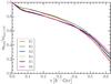 |
Fig. 15 Fraction of remaining ISM bound to the galaxy compared to the initial value is shown. In the runs with lower resolution, less gas is stripped at the beginning in the outskirts of the galaxy cluster, but more gas is stripped at pericentre passage. |
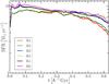 |
Fig. 16 Star formation rate of runs with different resolution are shown for the interaction of galaxy G1a with cluster A. Higher resolution leads to higher SFR. The SFR clearly converges with increasing resolution. |
First, we check the ICM properties along the trajectory of the galaxy within the galaxy cluster. In Fig. 14 we show relative velocity, density, corresponding ram pressure, and temperature of the ICM in front of the galaxy. The low resolution runs R1-R2 show a substantial scatter in velocity and temperature at the beginning of the simulation. The initial ICM resolution at that quite low density is very low in those runs and hence gas cells cannot be refined fast enough. Furthermore, the peak of ram pressure is shifted in time by about 20 h-1Myr. On the other hand, the medium (R3−R6) and high resolution (R7) runs are in very good agreement.
The amount of stripped gas for different resolutions is shown in Fig. 15. As in the wind-tunnel experiments of Heß & Springel (2012), stripping becomes less efficient with increasing resolution. Reassuringly, the amount of stripped gas is however in good agreement especially for the medium and high resolution run. Even at pericentre passage, the amount of stripped gas differs by only a few percent. Interestingly, the low resolution runs show less gas stripping in the outer parts of the cluster at low ICM densities. Afterwards, however, as expected more gas is stripped as the ICM density gets higher.
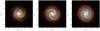 |
Fig. 17 Convergence of mock images of the galaxy G1 after 600 h-1 Myr of evolution in the galaxy cluster for run R1, R3, and R6 (from left to right), respectively. |
The SFR for the distinct runs is shown in Fig. 16. As expected from simulations of model galaxies in isolation (Springel & Hernquist 2003; Springel 2005; Heß & Springel 2012), SF is enhanced and converges with increasing resolution in our new simulation set-up as well. The target volume of the ICM has no influence on the SFR of the galaxy. On the other hand, at pericentre passage, when the galaxy has a very high relative velocity, the SFR is lower when the gas cells in front of the galaxy are refined to the target volume immediately before the galaxy passes by. This effect is evident in both low and medium resolution runs (R1−R2 and R3−R5).
Related to SFR and morphology of the galaxy with different resolutions, in Fig. 17 we provide mock colour images of the galaxy for run R1, R3, and R6 after 600 h-1 Myr of evolution in the galaxy cluster. As the SFR is enhanced with higher resolution, the galaxy appears bluer in R6 but redder in R1. Furthermore, structural features, such as spiral arms, are much more pronounced at higher resolution.
These tests hence show that the new refinement strategy, which is crucial to carry out high resolution RPS simulations in realistic live models of galaxy clusters, is valid and working well. There is no influence on the amount of stripped gas when the refinement is applied. In particular, there is no relevant difference in the mixing of the gas with the ICM, and SF in the wake is not prevented either. The higher amount of gas in the star-forming regime is mostly present in the disk itself, as less gas is dragged from the outskirts of the disk because of the higher resolved cells present there. Furthermore, it is very important that the gas in front of the galaxies is refined sufficiently in advance, which is an issue especially when the galaxy moves fast. This is ensured in all of our production runs.
5. Conclusions
In this work, we introduced a new set-up for realistic ram-pressure stripping simulations that employs the moving-mesh code AREPO combined with a special refinement strategy to cope with the high dynamic range in density encountered in this problem and the need to restrict the high resolution to the path of the galaxy for reasons of computational efficiency. In addition, we prevented radiative cooling in the background cluster and the computational cost this would entail through a suitable marker field. With our approach, the interaction of a live galaxy cluster with an infalling galaxy can be followed at high resolution.
We constructed several different galaxy models, including variations of the amount of gas in the halos of the galaxies, and collided these models with galaxy clusters of different mass. We then analysed the evolution of SFR, galaxy colours, and bound baryonic masses to the galaxies in comparison to control simulations carried out in isolation. Through extensive convergence tests we verified that all our conclusions are numerically robust.
In general, we find that the cold disks of our model galaxies are remarkably resilient against RPS, unless the pericentre distance of their orbit is very small and the encounter is “deep”. Typically, the galaxies continue to form stars with only slightly modified rates as a result of the environmental interaction, and in some cases, they even show an enhanced SFR. These modifications primarily result from a stripping of the hot gaseous halos of the galaxies and, in some cases, from a compression of the ISM of the disks. We confirm that the inclination angle has only a moderate influence on the overall strength of the stripping process. The colour evolution of our galaxies, augmented with sensible assumptions about their initial age, is in good agreement with observational data.
In particular, quenching timescales do not differ significantly from isolation (τquench> 1 h-1 Gyr). Inefficient stripping is balanced by increased SF in the RP compressed disk. Hence, the influence of RPS on galaxy quenching is mainly due to the missing gas supply from the gas halo. Only extreme, supposedly rare cases of RPS in the centre of massive clusters are able to completely strip the gas disk and quench SF on short timescales of a few hundred Myr.
Furthermore, as predicted by findings of wind-tunnel simulations, the turbulent wake of the stripped galaxies is narrower in our simulations, which include radiative cooling for the ISM, compared to previous studies of RPS in live galaxy clusters, which only implemented adiabatic gas physics. The stripped gas is heated up and diluted quickly to background temperature and density and is thus free of SF. The metallicity of stripped gas can reach near solar values but is diluted fast because of high relative velocities. After cluster passage, in all of the scenarios metallicity in stripped gas is mostly identical, although the stripped metal mass can differ by a factor of eight.
When compared to commonly employed semi-analytic prescriptions for RPS, we find that our simulations in general show less stripping than inferred in SAMs with the exact size of the mismatch depending on the details of the employed SAM. It thus seems clear that the widely reported difficulty of SAMs to account for relatively blue galaxies in dense environments may largely be a result of an inaccurate treatment of RPS. The work presented here should be helpful in re-calibrating the corresponding model prescriptions and putting them on a quantitatively more accurate physical basis, such that one can continue to use SAMs as a shortcut for the expensive but more reliable full hydrodynamical simulations.
Acknowledgments
D.S. thanks Federico Marinacci, Markus Haider, Matteo Bianconi, Andreas Bauer, Kevin Schaal, and Rüdiger Pakmor for many valuable discussions. D.S. acknowledges support of the Austrian Federal Ministry of Science, Research and Economy through the Uni-Infrastrukturprogramm of the Focal Point Scientific Computing at the University of Innsbruck, the doctoral school Computational Interdisciplinary Modelling FWF DK plus (W1227), the research grant from the office of the vice rector for research of the University of Innsbruck, and the award for research stay abroad of the International Relations Office of the University of Innsbruck. V.S. acknowledges support through the European Research Council through ERC-StG grant EXAGAL-308037 and the Klaus Tschira Foundation. Furthermore, we would like to acknowledge the valuable comments of the anonymous referee.
References
- Abramson, A., & Kenney, J. D. P. 2014, AJ, 147, 63 [NASA ADS] [CrossRef] [Google Scholar]
- Asplund, M., Grevesse, N., & Sauval, A. J. 2005, in Cosmic Abundances as Records of Stellar Evolution and Nucleosynthesis, eds. T. G. Barnes, III & F. N. Bash, ASP Conf. Ser., 336, 25 [Google Scholar]
- Athanassoula, E. 2005, MNRAS, 358, 1477 [NASA ADS] [CrossRef] [Google Scholar]
- Bekki, K. 2009, MNRAS, 399, 2221 [NASA ADS] [CrossRef] [Google Scholar]
- Benson, A. J. 2012, New Astron., 17, 175 [Google Scholar]
- Bischko, J. C., Steinhauser, D., & Schindler, S. 2015, A&A, 576, A76 [NASA ADS] [CrossRef] [EDP Sciences] [Google Scholar]
- Boissier, S., Boselli, A., Duc, P.-A., et al. 2012, A&A, 545, A142 [NASA ADS] [CrossRef] [EDP Sciences] [Google Scholar]
- Boselli, A., & Gavazzi, G. 2006, PASP, 118, 517 [NASA ADS] [CrossRef] [Google Scholar]
- Boselli, A., Gavazzi, G., Lequeux, J., et al. 1997, A&A, 327, 522 [NASA ADS] [Google Scholar]
- Boselli, A., Boissier, S., Cortese, L., & Gavazzi, G. 2009, Astron. Nachr., 330, 904 [NASA ADS] [CrossRef] [Google Scholar]
- Bresolin, F., Kennicutt, R. C., & Ryan-Weber, E. 2012, ApJ, 750, 122 [NASA ADS] [CrossRef] [Google Scholar]
- Chung, A., van Gorkom, J. H., Kenney, J. D. P., Crowl, H., & Vollmer, B. 2009, AJ, 138, 1741 [NASA ADS] [CrossRef] [Google Scholar]
- Conroy, C., & Gunn, J. E. 2010, ApJ, 712, 833 [NASA ADS] [CrossRef] [Google Scholar]
- Conroy, C., Gunn, J. E., & White, M. 2009, ApJ, 699, 486 [NASA ADS] [CrossRef] [Google Scholar]
- Cora, S. A. 2006, MNRAS, 368, 1540 [Google Scholar]
- Cortese, L., Marcillac, D., Richard, J., et al. 2007, MNRAS, 376, 157 [NASA ADS] [CrossRef] [Google Scholar]
- De Lucia, G., Kauffmann, G., & White, S. D. M. 2004, MNRAS, 349, 1101 [NASA ADS] [CrossRef] [Google Scholar]
- Domainko, W., Mair, M., Kapferer, W., et al. 2006, A&A, 452, 795 [NASA ADS] [CrossRef] [EDP Sciences] [Google Scholar]
- Duc, P.-A., Brinks, E., Springel, V., et al. 2000, AJ, 120, 1238 [NASA ADS] [CrossRef] [Google Scholar]
- Ebeling, H., Stephenson, L. N., & Edge, A. C. 2014, ApJ, 781, L40 [NASA ADS] [CrossRef] [Google Scholar]
- Eke, V. R., Navarro, J. F., & Frenk, C. S. 1998, ApJ, 503, 569 [NASA ADS] [CrossRef] [Google Scholar]
- Feldmann, R., & Mayer, L. 2015, MNRAS, 446, 1939 [NASA ADS] [CrossRef] [Google Scholar]
- Ferguson, A. M. N., Gallagher, J. S., & Wyse, R. F. G. 1998, AJ, 116, 673 [NASA ADS] [CrossRef] [Google Scholar]
- Font, A. S., Bower, R. G., McCarthy, I. G., et al. 2008, MNRAS, 389, 1619 [NASA ADS] [CrossRef] [Google Scholar]
- Fryxell, B., Olson, K., Ricker, P., et al. 2000, ApJS, 131, 273 [NASA ADS] [CrossRef] [Google Scholar]
- Fumagalli, M., Fossati, M., Hau, G. K. T., et al. 2014, MNRAS, 445, 4335 [NASA ADS] [CrossRef] [Google Scholar]
- Guedes, J., Callegari, S., Madau, P., & Mayer, L. 2011, ApJ, 742, 76 [NASA ADS] [CrossRef] [MathSciNet] [Google Scholar]
- Gunn, J. E., & Gott, III, J. R. 1972, ApJ, 176, 1 [NASA ADS] [CrossRef] [Google Scholar]
- Guo, Q., White, S., Boylan-Kolchin, M., et al. 2011, MNRAS, 413, 101 [NASA ADS] [CrossRef] [Google Scholar]
- Guo, Q., Cole, S., Eke, V., Frenk, C., & Helly, J. 2013, MNRAS, 434, 1838 [NASA ADS] [CrossRef] [Google Scholar]
- Hernquist, L. 1990, ApJ, 356, 359 [NASA ADS] [CrossRef] [Google Scholar]
- Heß, S., & Springel, V. 2010, MNRAS, 406, 2289 [NASA ADS] [CrossRef] [Google Scholar]
- Heß, S., & Springel, V. 2012, MNRAS, 426, 3112 [NASA ADS] [CrossRef] [Google Scholar]
- Hester, J. A., Seibert, M., Neill, J. D., et al. 2010, ApJ, 716, L14 [NASA ADS] [CrossRef] [Google Scholar]
- Höller, H., Stöckl, J., Benson, A., et al. 2014, A&A, 569, A31 [NASA ADS] [CrossRef] [EDP Sciences] [Google Scholar]
- Jáchym, P., Palouš, J., Köppen, J., & Combes, F. 2007, A&A, 472, 5 [NASA ADS] [CrossRef] [EDP Sciences] [Google Scholar]
- Jáchym, P., Köppen, J., Palouš, J., & Combes, F. 2009, A&A, 500, 693 [NASA ADS] [CrossRef] [EDP Sciences] [Google Scholar]
- Kapferer, W., Sluka, C., Schindler, S., Ferrari, C., & Ziegler, B. 2009, A&A, 499, 87 [NASA ADS] [CrossRef] [EDP Sciences] [Google Scholar]
- Katz, N., Weinberg, D. H., & Hernquist, L. 1996, ApJS, 105, 19 [NASA ADS] [CrossRef] [Google Scholar]
- Kauffmann, G., Li, C., Zhang, W., & Weinmann, S. 2013, MNRAS, 430, 1447 [NASA ADS] [CrossRef] [Google Scholar]
- Kenney, J. D. P., Geha, M., Jáchym, P., et al. 2014, ApJ, 780, 119 [NASA ADS] [CrossRef] [Google Scholar]
- Kennicutt, Jr., R. C. 1998, ApJ, 498, 541 [NASA ADS] [CrossRef] [Google Scholar]
- Kimm, T., Somerville, R. S., Yi, S. K., et al. 2009, MNRAS, 394, 1131 [NASA ADS] [CrossRef] [Google Scholar]
- Kronberger, T., Kapferer, W., Ferrari, C., Unterguggenberger, S., & Schindler, S. 2008, A&A, 481, 337 [NASA ADS] [CrossRef] [EDP Sciences] [Google Scholar]
- Lagos, C. D. P., Cora, S. A., & Padilla, N. D. 2008, MNRAS, 388, 587 [NASA ADS] [CrossRef] [Google Scholar]
- Lanzoni, B., Guiderdoni, B., Mamon, G. A., Devriendt, J., & Hatton, S. 2005, MNRAS, 361, 369 [NASA ADS] [CrossRef] [Google Scholar]
- Larson, R. B., Tinsley, B. M., & Caldwell, C. N. 1980, ApJ, 237, 692 [NASA ADS] [CrossRef] [Google Scholar]
- Lupton, R., Blanton, M. R., Fekete, G., et al. 2004, PASP, 116, 133 [NASA ADS] [CrossRef] [Google Scholar]
- Marinacci, F., Pakmor, R., & Springel, V. 2014, MNRAS, 437, 1750 [NASA ADS] [CrossRef] [Google Scholar]
- McCarthy, I. G., Frenk, C. S., Font, A. S., et al. 2008, MNRAS, 383, 593 [NASA ADS] [CrossRef] [Google Scholar]
- McPartland, C., Ebeling, H., Roediger, E., & Blumenthal, K. 2016, MNRAS, 455, 2994 [NASA ADS] [CrossRef] [Google Scholar]
- Merluzzi, P., Busarello, G., Dopita, M. A., et al. 2013, MNRAS, 429, 1747 [NASA ADS] [CrossRef] [Google Scholar]
- Mo, H. J., Mao, S., & White, S. D. M. 1998, MNRAS, 295, 319 [Google Scholar]
- Moster, B. P., Macciò, A. V., Somerville, R. S., Naab, T., & Cox, T. J. 2011, MNRAS, 415, 3750 [NASA ADS] [CrossRef] [Google Scholar]
- Murante, G., Monaco, P., Borgani, S., et al. 2015, MNRAS, 447, 178 [NASA ADS] [CrossRef] [Google Scholar]
- Navarro, J. F., Frenk, C. S., & White, S. D. M. 1996, ApJ, 462, 563 [NASA ADS] [CrossRef] [Google Scholar]
- Nelson, D., Genel, S., Vogelsberger, M., et al. 2015, MNRAS, 448, 59 [NASA ADS] [CrossRef] [Google Scholar]
- Neto, A. F., Gao, L., Bett, P., et al. 2007, MNRAS, 381, 1450 [NASA ADS] [CrossRef] [Google Scholar]
- Nulsen, P. E. J. 1982, MNRAS, 198, 1007 [NASA ADS] [CrossRef] [Google Scholar]
- O’Shea, B. W., Bryan, G., Bordner, J., et al. 2004, ArXiv e-prints [arXiv:astro-ph/0403044] [Google Scholar]
- Ott, F., & Schnetter, E. 2003, ArXiv e-prints [arXiv:physics/0303112] [Google Scholar]
- Owen, F. N., Keel, W. C., Wang, Q. D., Ledlow, M. J., & Morrison, G. E. 2006, AJ, 131, 1974 [NASA ADS] [CrossRef] [Google Scholar]
- Owers, M. S., Couch, W. J., Nulsen, P. E. J., & Randall, S. W. 2012, ApJ, 750, L23 [NASA ADS] [CrossRef] [Google Scholar]
- Pakmor, R., Kromer, M., Taubenberger, S., & Springel, V. 2013, ApJ, 770, L8 [NASA ADS] [CrossRef] [Google Scholar]
- Peng, Y.-J., Lilly, S. J., Kovač, K., et al. 2010, ApJ, 721, 193 [NASA ADS] [CrossRef] [Google Scholar]
- Pranger, F., Böhm, A., Ferrari, C., et al. 2014, A&A, 570, A40 [NASA ADS] [CrossRef] [EDP Sciences] [Google Scholar]
- Querejeta, M., Eliche-Moral, M. C., Tapia, T., et al. 2015, A&A, 573, A78 [NASA ADS] [CrossRef] [EDP Sciences] [Google Scholar]
- Read, J. I., Hayfield, T., & Agertz, O. 2010, MNRAS, 405, 1513 [NASA ADS] [Google Scholar]
- Roediger, E., & Brüggen, M. 2006, MNRAS, 369, 567 [NASA ADS] [CrossRef] [Google Scholar]
- Roediger, E., & Brüggen, M. 2007, MNRAS, 380, 1399 [NASA ADS] [CrossRef] [Google Scholar]
- Roediger, E., & Brüggen, M. 2008, MNRAS, 388, 465 [NASA ADS] [CrossRef] [Google Scholar]
- Roediger, E., & Hensler, G. 2005, A&A, 433, 875 [NASA ADS] [CrossRef] [EDP Sciences] [Google Scholar]
- Roediger, E., Brüggen, M., & Hoeft, M. 2006, MNRAS, 371, 609 [NASA ADS] [CrossRef] [Google Scholar]
- Ruszkowski, M., Brüggen, M., Lee, D., & Shin, M.-S. 2014, ApJ, 784, 75 [NASA ADS] [CrossRef] [Google Scholar]
- Salpeter, E. E. 1955, ApJ, 121, 161 [Google Scholar]
- Schawinski, K., Urry, C. M., Simmons, B. D., et al. 2014, MNRAS, 440, 889 [NASA ADS] [CrossRef] [Google Scholar]
- Schindler, S. 2007, in EAS PS 24, eds. E. Emsellem, H. Wozniak, G. Massacrier, J.-F. Gonzalez, J. Devriendt, & N. Champavert, 121 [Google Scholar]
- Schindler, S., Kapferer, W., Domainko, W., et al. 2005, A&A, 435, L25 [NASA ADS] [CrossRef] [EDP Sciences] [Google Scholar]
- Scott, T. C., Bravo-Alfaro, H., Brinks, E., et al. 2010, MNRAS, 403, 1175 [NASA ADS] [CrossRef] [Google Scholar]
- Shu, F. H. 1992, Physics of Astrophysics, Vol. II (University Science Books) [Google Scholar]
- Springel, V. 2005, MNRAS, 364, 1105 [NASA ADS] [CrossRef] [Google Scholar]
- Springel, V. 2010, MNRAS, 401, 791 [NASA ADS] [CrossRef] [Google Scholar]
- Springel, V., & Hernquist, L. 2003, MNRAS, 339, 289 [Google Scholar]
- Springel, V., & White, S. D. M. 1999, MNRAS, 307, 162 [NASA ADS] [CrossRef] [Google Scholar]
- Springel, V., Di Matteo, T., & Hernquist, L. 2005, MNRAS, 361, 776 [NASA ADS] [CrossRef] [Google Scholar]
- Steinhauser, D., Haider, M., Kapferer, W., & Schindler, S. 2012, A&A, 544, A54 [NASA ADS] [CrossRef] [EDP Sciences] [Google Scholar]
- Sun, M. 2012, New J. Phys., 14, 045004 [NASA ADS] [CrossRef] [Google Scholar]
- Tecce, T. E., Cora, S. A., Tissera, P. B., Abadi, M. G., & Lagos, C. D. P. 2010, MNRAS, 408, 2008 [NASA ADS] [CrossRef] [Google Scholar]
- Tonnesen, S., & Bryan, G. L. 2008, ApJ, 684, L9 [NASA ADS] [CrossRef] [Google Scholar]
- Tonnesen, S., & Bryan, G. L. 2010, ApJ, 709, 1203 [NASA ADS] [CrossRef] [Google Scholar]
- Tonnesen, S., & Bryan, G. L. 2012, MNRAS, 422, 1609 [NASA ADS] [CrossRef] [Google Scholar]
- van Leer, B. 1984, SIAM J. Sci. Stat. Comput., 5, 1 [Google Scholar]
- van Leer, B. 2006, Comm. Comput. Phys., 1, 192 [Google Scholar]
- Vazza, F. 2011, MNRAS, 410, 461 [NASA ADS] [CrossRef] [Google Scholar]
- Vogelsberger, M., Sijacki, D., Kereš, D., Springel, V., & Hernquist, L. 2012, MNRAS, 425, 3024 [NASA ADS] [CrossRef] [Google Scholar]
- Vollmer, B., Braine, J., Balkowski, C., Cayatte, V., & Duschl, W. J. 2001a, A&A, 374, 824 [NASA ADS] [CrossRef] [EDP Sciences] [Google Scholar]
- Vollmer, B., Cayatte, V., Balkowski, C., & Duschl, W. J. 2001b, ApJ, 561, 708 [NASA ADS] [CrossRef] [Google Scholar]
- Wang, W., Sales, L. V., Henriques, B. M. B., & White, S. D. M. 2014, MNRAS, 442, 1363 [NASA ADS] [CrossRef] [Google Scholar]
- Weinmann, S. M., van den Bosch, F. C., Yang, X., & Mo, H. J. 2006, MNRAS, 366, 2 [NASA ADS] [CrossRef] [Google Scholar]
- Weinmann, S. M., Kauffmann, G., von der Linden, A., & De Lucia, G. 2010, MNRAS, 406, 2249 [NASA ADS] [CrossRef] [Google Scholar]
- Werner, N., Durret, F., Ohashi, T., Schindler, S., & Wiersma, R. P. C. 2008, Space Sci. Rev., 134, 337 [NASA ADS] [CrossRef] [Google Scholar]
- Yagi, M., Yoshida, M., Komiyama, Y., et al. 2010, AJ, 140, 1814 [NASA ADS] [CrossRef] [Google Scholar]
- Yoshida, M., Yagi, M., Komiyama, Y., et al. 2008, ApJ, 688, 918 [NASA ADS] [CrossRef] [Google Scholar]
- Yurin, D., & Springel, V. 2014, MNRAS, 444, 62 [NASA ADS] [CrossRef] [Google Scholar]
- Zaritsky, D., Kennicutt, Jr., R. C., & Huchra, J. P. 1994, ApJ, 420, 87 [NASA ADS] [CrossRef] [Google Scholar]
- Zhang, Y.-Y., Laganá, T. F., Pierini, D., et al. 2011, A&A, 535, A78 [NASA ADS] [CrossRef] [EDP Sciences] [Google Scholar]
All Tables
Initial properties of the two primary galaxy models G1 and G2 used in this study.
All Figures
|
Fig. 1 a) Radial density profiles of the gas (solid lines) and DM (dashed lines) of the galaxy cluster models used in this study. The profiles are shown at the beginning of the galaxy interaction, after the cluster models were allowed to relax for ~1 Gyr. Vertical dotted lines indicate the virial radius r200 for clusters A, B, and C, from right to left. b) Corresponding temperature profiles of the ICM. |
| In the text | |
|
Fig. 2 Fiducial galaxy orbits adopted for studying the interaction of galaxy model G1a with the three different galaxy clusters constructed for the study. a) Trajectories of the galaxy in clusters A, B, and C, scaled to the virial radius of the corresponding cluster. b) Time evolution of the distance of the galaxy to the corresponding cluster centre. c) Effective inclination angle of the galaxy (angle between the spin vector of the disk and its instantaneous velocity vector). |
| In the text | |
|
Fig. 3 Physical conditions encountered by galaxy G1 as it falls into different galaxy clusters. The top left panel shows the relative velocity of the galaxy, the top right panel shows the ICM density, the bottom left panel gives the resulting ram pressure Pram, and the bottom right panel indicates the ICM temperature encountered by galaxy G1a for runs S1, S3, and S4, respectively. Galaxy inclination does not affect these values significantly, hence run S2 looks essentially the same as S1 and is hence not shown. Also, as in Fig. 2, the values for galaxy G2 in runs S5−S7 are very similar as the trajectories are nearly the same. |
| In the text | |
|
Fig. 4 a) Star formation rate of model galaxy G1 when evolved in isolation. The three variants shown correspond to different gas masses in the corona. Model G1a has the same baryonic mass in the halo as in the disk, G1b has half of that mass, and G1c has only 1% of the disk mass in the gaseous halo. b) Evolution of different baryonic components of galaxy model G1a (solid lines) and G1c (dashed lines) evolved in isolation. The red line indicates accreted halo mass onto the disk. The mass components shown are newly formed stars, star-forming (ρ> 2.6 h2 cm-3), and non-star-forming gas. The black line shows the total gas mass in the disk plus newly formed stars. |
| In the text | |
|
Fig. 5 Ram-pressure stripping of galaxy G1a for runs S1−S4 in the corresponding clusters. The panels of the column on the right-hand side show gas surface density profiles of the galaxy (solid lines) and exponential surface density fits based on the gas mass in the galaxy at a particular timestep (dotted lines) as coded by the colours. Vertical dashed lines indicate the radius, at which the actual surface density drops more than one dex below the exponential fit. The panels of the middle column give the evolution of the stripping radius in the simulations, which are determined with three different measurement methods (defined in Sect. 3.2). The blue shaded area encloses the minimum and maximum stripping radius, calculated by different theoretical predictions based on the standard Gunn & Gott (1972) criterion (blue dashed line), considering initial or current and total disk mass, the inclination of the galaxy as well as Rankine-Hugoniot post-shock conditions. The black lines in the panels of the left column show the effective mass lost via stripping in the simulations. The edges of the blue shaded region indicate the minimum and maximum mass loss, considering the stripping radius calculated with the different models. The red shaded area depicts the corresponding extrema of mass loss due to a continuous stripping assumption. The yellow dashed lines indicate the model that best fits the corresponding simulation. |
| In the text | |
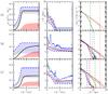 |
Fig. 6 Same as Fig. 5 but for galaxy G2. |
| In the text | |
|
Fig. 7 Slices of thickness 0.2 h-1 kpc and extension 100 h-1 kpc × 40 h-1 kpc through the galaxy and its wake in run S1, after 600 h-1Myr of evolution. Quantities are mapped using an SPH kernel. The different panels show: a) gas density, b) velocity magnitude, c) metallicity, d) temperature, and e) vorticity magnitude. |
| In the text | |
|
Fig. 8 Panels a) and b): evolution of metal mass in both model galaxies as a function of simulation time for interactions with clusters A or B, respectively. The solid lines indicate the metal mass in both gas and newly formed stars that are gravitationally bound to the galaxy, whereas the dashed lines give the metal mass locked up only in newly formed stars. The dotted lines indicate the metal mass in the stripped gas wake. Panel c): metallicity histograms of stripped gas (considering gas cells not gravitationally bound to the galaxy anymore and with ISM mass fraction >1%) as a function of time. The colour encodes the mass fraction in each metallicity bin of the total gas mass stripped for each timestep. The black solid line shows the mean metallicity value of the gas cells in the histogram, while the dashed line indicates Z⊙. |
| In the text | |
|
Fig. 9 a), b) Evolution of the |
| In the text | |
|
Fig. 10 Colour evolution (in the u-i index of the SDSS) of galaxies G1 (top panel) and G2 (bottom panel) as a function of time while interacting with different cluster environments. The slow evolution towards redder colours in the interactions with clusters B and C is actually very similar to the evolution of the galaxies in isolation, showing that the gas consumption timescale is not significantly affected by RPS in these models. This is different in the deep interaction with cluster A, where a rapid shutdown of SF is achieved. |
| In the text | |
|
Fig. 11 Colour–colour diagrams showing the evolution of galaxies in NUV-u vs. u-r space as they interact with different clusters. The top panel is for model galaxy G1, and the bottom panel for G2. The colour is indicating different environments as shown in the legend. Stars mark simulation times with their brightness encoding 0, 0.5, 1.5 and 2 h-1 Gyr (the brightness corresponds to the one used for the big squares in Figs. 9a and b). The grey shaded contours represent the densities of the observed early- (upper right concentration) and late-type (lower left peak) galaxy populations, as determined by Schawinski et al. (2014). |
| In the text | |
|
Fig. 12 Mock colour images of galaxy G1a in different environments. The evolution in isolation and runs S1, S3 and S4 are depicted in the different rows. In each column, the state at a selected time (indicated on top) is shown for each simulation. |
| In the text | |
|
Fig. 13 Comparison of the simulations with SAM expectations. a) The SFR of galaxy G1a in cluster A, B, and C (runs S1, S3, and S4, respectively) and galaxy G1c is depicted with solid lines. The dashed lines correspond to the SFR of galaxy G1c with standard prescriptions for RPS (Gunn & Gott 1972) and SF (Cora 2006). In b), the same comparison is shown for the time evolution of the galaxy colours. |
| In the text | |
|
Fig. 14 Convergence study of the time evolution of the ICM properties measured in the surrounding and 45 h-1 kpc in front of the galaxy. |
| In the text | |
|
Fig. 15 Fraction of remaining ISM bound to the galaxy compared to the initial value is shown. In the runs with lower resolution, less gas is stripped at the beginning in the outskirts of the galaxy cluster, but more gas is stripped at pericentre passage. |
| In the text | |
|
Fig. 16 Star formation rate of runs with different resolution are shown for the interaction of galaxy G1a with cluster A. Higher resolution leads to higher SFR. The SFR clearly converges with increasing resolution. |
| In the text | |
|
Fig. 17 Convergence of mock images of the galaxy G1 after 600 h-1 Myr of evolution in the galaxy cluster for run R1, R3, and R6 (from left to right), respectively. |
| In the text | |
Current usage metrics show cumulative count of Article Views (full-text article views including HTML views, PDF and ePub downloads, according to the available data) and Abstracts Views on Vision4Press platform.
Data correspond to usage on the plateform after 2015. The current usage metrics is available 48-96 hours after online publication and is updated daily on week days.
Initial download of the metrics may take a while.