| Issue |
A&A
Volume 591, July 2016
|
|
|---|---|---|
| Article Number | A38 | |
| Number of page(s) | 18 | |
| Section | Extragalactic astronomy | |
| DOI | https://doi.org/10.1051/0004-6361/201527618 | |
| Published online | 08 June 2016 | |
Robust automatic photometry of local galaxies from SDSS
Dissecting the color magnitude relation with color profiles⋆
1 Dipartimento di Fisica G. Occhialini, Università di Milano-Bicocca, Piazza della Scienza 3, 20126 Milano, Italy
e-mail: This email address is being protected from spambots. You need JavaScript enabled to view it.
2 Institute for Computational Cosmology and Centre for Extragalactic Astronomy, Department of Physics, Durham University, South Road, Durham DH1 3LE, UK
3 Universitäts-Sternwarte München, Scheinerstrasse 1, 81679 München, Germany
4 Max-Planck-Institut für Extraterrestrische Physik, Giessenbachstrasse, 85748 Garching, Germany
Received: 22 October 2015
Accepted: 23 March 2016
Abstract
We present an automatic procedure to perform reliable photometry of galaxies on SDSS images. We selected a sample of 5853 galaxies in the Coma and Virgo superclusters. For each galaxy, we derive Petrosian g and i magnitudes, surface brightness and color profiles. Unlike the SDSS pipeline, our procedure is not affected by the well known shredding problem and efficiently extracts Petrosian magnitudes for all galaxies. Hence we derived magnitudes even from the population of galaxies missed by the SDSS which represents ~25% of all local supercluster galaxies and ~95% of galaxies with g < 11 mag. After correcting the g and i magnitudes for Galactic and internal extinction, the blue and red sequences in the color magnitude diagram are well separated, with similar slopes. In addition, we study (i) the color-magnitude diagrams in different galaxy regions, the inner (r ≤ 1 kpc), intermediate (0.2RPet ≤ r ≤ 0.3RPet) and outer, disk-dominated (r ≥ 0.35RPet)) zone; and (ii), we compute template color profiles, discussing the dependences of the templates on the galaxy masses and on their morphological type. The two analyses consistently lead to a picture where elliptical galaxies show no color gradients, irrespective of their masses. Spirals, instead, display a steeper gradient in their color profiles with increasing mass, which is consistent with the growing relevance of a bulge and/or a bar component above 1010 M⊙.
Key words: galaxies: evolution / galaxies: fundamental parameters / galaxies: star formation / galaxies: photometry
Full Table A.1 is only available at the CDS via anonymous ftp to cdsarc.u-strasbg.fr (130.79.128.5) or via http://cdsarc.u-strasbg.fr/viz-bin/qcat?J/A+A/591/A38
© ESO, 2016
1. Introduction
The advent of the Sloan Digital Sky Survey (SDSS, York et al. 2000) represents a revolution in many fields of observational astronomy. The final SDSS catalog consists of about 500 million photometric objects in five bands with more than 1 million spectra. This huge amount of publicly available data has given the community the unprecedented opportunity to study galaxy properties from a statistical point of view in many different regimes of local density and cosmic epochs.
Early multi-wavelength studies by Faber (1973), Visvanathan & Sandage (1977), Aaronson et al. (1981) suggested the existence for E and S0s of a color-magnitude relation with a shallow slope and a small intrinsic scatter. Similarly, other authors stated that spiral galaxies follow a color magnitude relation with a much greater intrinsic scatter (Chester & Roberts 1964; Visvanathan & Griersmith 1977; Griersmith 1980). However these pioneering studies were based on limited samples of only tens or at most hundreds of objects which prevented conclusive statistical analyses. It was only with the advent of the SDSS that Strateva et al. (2001), using an unprecedented sample of 147 920 galaxies, have definitely demonstrated the bimodal distribution of galaxy colors and luminosity, with a clear separation between star-forming blue late-type galaxies and passive, red and dead galaxies. Since 2001, this bimodality in galaxy distribution has been observed in many different regimes of density (Baldry et al. 2004; Kauffmann et al. 2004; Gavazzi et al. 2010) at different redshifts (Bell et al. 2004; Xue et al. 2010) suggesting an evolutionary path of galaxies from the so-called blue cloud of star forming galaxies to the red sequence of dead galaxies. However, the mechanisms that make galaxies depart from the blue cloud to reach the red sequence (star formation-quenching) are still under scrutiny.
However the SDSS pipeline was optimized for the extraction of photometric parameters of galaxies at the median redshift of the survey (z ~ 0.1). Large nearby galaxies, often exceeding the apparent diameter of few arcmins were obviously penalized by this choice. One longstanding problem that affects the identification of extended sources (Blanton et al. 2005) is the so-called shredding of large, bright (in apparent magnitude) galaxies by the automatic pipelines, leading to wrong detections and incorrect magnitude calculations. Moreover, restrictions due to fiber collisions dictate that no two fibers can be placed closer than 55 arcsec during the same observation (Blanton et al. 2003) which affects the spectroscopy of crowded environments and introduces incompleteness at z< 0.03 where many local large scale structures exist, namely the local and the Coma superclusters (see Fig. 1).
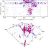 |
Fig. 1 Sky projection (top) and Wedge diagram (bottom) of galaxies belonging to the sample studied in this work: the Coma supercluster (δ> 18°; cz> 4000 km s-1) and the local supercluster (δ< 18°; cz< 3000 km s-1). Blue dots represent late type galaxies (LTGs) while red dots stand for early type galaxies (ETGs). The dotted rectangular regions indicate the areas surveyed by ALFALFA. |
Nevertheless, galaxies of the local Universe are, at fixed luminosity, the brightest as well as the best spatially resolved objects of the sky. Therefore, within the SDSS, local galaxies can be analyzed down to a mass limit that cannot be reached at higher redshift and, in addition, their structures and morphology are easier to constrain. In fact the median resolution of the SDSS, given by the median point spread function (PSF ~1.4 arcsec, in the r-band), corresponds to a physical scale of ~600 pc at the distance of the Coma cluster (~95.38 Mpc) and ~80 pc at the distance of Virgo (~17 Mpc, Gavazzi et al. 1999; Mei et al. 2007). This resolution is sufficient to resolve even small structures such as nuclear disks in galaxies.
Henceforth local galaxies are a natural test-bed for studies on the evolution of structures at higher redshift. The Local and Coma superclusters contain thousands of galaxies and are a perfect laboratory for studying the leading processes that transform galaxies from star forming objects into red and dead structures. Moreover the nearby Universe contain a wide range of environments that have been broadly studied by many groups at different wavelengths (Haynes et al. 2011; Boselli et al. 2011; Gavazzi et al. 2010, 2012). These regions are therefore perfect to constrain the properties of galactic structures in different environments at different wavelengths, with the SDSS magnitudes playing a fundamental role in the panchromatic description of these structures. Both areas of the sky have been fully covered by the SDSS in its five optical filters (u, g, r, i, z) and the data have been first published in the data release 4 (DR4) for (Virgo, Adelman-McCarthy et al. 2006) and in the DR7 (Coma, Abazajian et al. 2009). Unfortunately, the data of the Local and Coma clusters as given by SDSS are affected by the aforementioned difficulties of the SDSS pipeline and, despite the good quality of the data, many galaxies are not included in the catalogs or, if present, have in some cases unreliable photometry. Despite the fact that the worst photometric discrepancies affect only ~10% of the whole sample (see Sect. 4.1), these happen to coincide with the brightest galaxies in the Virgo and Coma clusters, thus affecting the high mass-end determination of the luminosity function that is already hampered by the lack of sampled volume.
In this context, our work aims to automatically generate high-quality photometry from SDSS imaging in two filters (g and i) for a sample of ~6000 galaxies within the local and Coma superclusters described in Sect. 2. Our IDL-based (Interactive Data Language) procedure is not limited to the magnitude extraction but performs aperture photometry in each considered band as well. In Sect. 3 we explain the method developed while in Sect. 4 we compare our magnitudes with the SDSS database, the Extended Virgo Cluster Catalog (Kim et al. 2014) and measurements from Gavazzi et al. (2012) and Gavazzi et al. (2013b). We test quantitatively the efficiency of the SDSS pipeline in these local clusters, while demonstrating the exquisite quality of our guided extraction. Sections 5−7 focus on the color-mass distribution of galaxies within our sample and on the properties of the different galactic components traced by color profiles as a function of mass and morphology. Our findings are discussed and summarized in Sects. 8 and 9.
2. The sample
This work is based on a sample of 6136 nearby galaxies in the spring sky selected from the SDSS as described in this section. The final sample is further split in two subsamples: i) the local supercluster (11h< RA < 16h; 0°< Dec < 18°; cz< 3000 km s-1) containing 1112 galaxies and includes the Virgo cluster; ii) the Coma supercluster (10h< RA < 16h; 18°< Dec < 32°; 4000 <cz< 9500 km s-1) containing 5024 galaxies and includes the Coma cluster. The two subsamples are displayed in Fig. 1.
Since galaxies at the distance of Virgo have apparent size often exceeding 5 arcmin, they are strongly affected by the shredding problem (Blanton et al. 2005) therefore our catalog cannot solely rely on the SDSS spectroscopic database. Thus, the local supercluster sample is selected following the prescriptions of Gavazzi et al. (2012): in the area occupied by the Virgo cluster, the selection is based on the VCC catalog (limited however to cz< 3000 km s-1) down to its magnitude completeness limit of 18 mag (Binggeli et al. 1985). The object selection is furthermore limited to objects with surface brightness above the 1σ of the mean sky surface brightness in i-band of the SDSS data (see Fig. 2). Outside the Virgo cluster the SDSS selection is complemented with objects taken from NED and ALFALFA (Haynes et al. 2011).
At the distance of the Coma supercluster the shredding problem is less severe and therefore we followed the selection of Gavazzi et al. (2010, 2013b). Briefly, galaxies are selected from the SDSS spectroscopic database DR7 (Abazajian et al. 2009) with r< 17.77 mag. To fill the residual incompleteness of the SDSS catalog for extended galaxies and due to fiber conflict, 133 galaxies from the CGCG catalog (Zwicky et al. 1968) with known redshifts from NED and 28 from ALFALFA are added, reaching a total of 5024 galaxies.
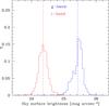 |
Fig. 2 Sky surface brightness distributions in g- (blue line) and i-band (red line) for the sample analyzed in this work. The vertical dashed lines indicate the mean surface brightness in g- and i-band respectively ⟨ Σi ⟩ = 24.36 ± 0.16 and ⟨ Σg ⟩ = 25.43 ± 0.17 mag arcsec-2. |
For these galaxies, we downloaded the SDSS images (using the online Mosaic service, see next section) in the g- and i-band. In this work, we test the procedure exclusively on these two bands for mainly two reason: i) the u and z filters have lower signal-to-noise ratio (S/N); ii) if compared to the i-band, the r filter have a central wavelength closer to the g filter central wavelength. Hence the g−i color is more sensitive to stellar population gradients and dust absorption. However only for 5753 (94%) targets the download process worked in both the i- and the g-band1. Of these, 221 galaxies were discarded a posteriori because they lie too close to bright stars or they have too low surface brightness (see Fig. 2). The remaining analyzed sample is constituted of 969 (local SC) + 4563 (Coma SC) objects, for a total of 5532 galaxies that can be considered representative of the nearby Universe. Their morphological classification and diameters are taken from the public database GOLDMine (Gavazzi et al. 2003, 2014b).
Summarizing, the sample analyzed in this work coincides with the one presented by Gavazzi et al. (2013b; with the selection criteria given in Gavazzi et al. 2010, Coma supercluster) and Gavazzi et al 2012 (local supercluster) except for 108 VCC galaxies that were excluded because their surface brightness (evaluated inside the radius at the 25th B-band isophote reported in GOLDMine) is lower than the mean sky surface brightness in i-band (Fig. 2). For the remaining 5532 galaxies the procedure developed in this work is aimed at obtaining more accurate photometry than reported in Gavazzi et al. (2012, 2013b).
3. The method
Our analysis code has been designed using IDL with the IDL Astronomy User’s Library (Landsman 1993) and takes advantage of Source Extractor (Bertin & Arnouts 1996). It processes FITS SDSS images in multiple bands that were downloaded using the IRSA and NVO image Mosaic service (Berriman et al. 2004; Katz et al. 2011). The Mosaic interface returns science-grade SDSS mosaics that preserve fluxes and astrometry and rectify backgrounds to a common level. Furthermore, the photon counts are normalized to a common exposure time of 1 s and the zero point is set to 28.03 mag in every filter. Images are centered on the target galaxies and span approximately three times their major diameter at the 25th magnitude arcsec-2V-band isophote as reported in GOLDMine (Gavazzi et al. 2003, 2014b). This ensures that a sufficient number of sky pixels exist around the targets for robust measurement of the sky background.
3.1. Image preparation, target detection and masking
The first step of the procedure is a preliminary estimate of the sky in each filter in a rectangular peripheral corona of width equal to one quarter of the full image size. This background mode value is subtracted from the images. The g and i sky-subtracted images are then averaged to create a higher signal-to-noise white frame that is analyzed using Source Extractor which detects and determines the photometric and geometric parameters of the objects in the field. We facilitated the Source Extractor detection enabling the filtering option of the routine. Each image is filtered with a Gaussian filter in order to smooth the image and avoid the detection of bright substructure inside the target galaxy as well as help the detection of the low surface brightness local supercluster irregular galaxies. In the Source Extractor setup that we adopted (for the technical details about the implementation we refer the reader to Appendices A and B) we apply a 13 × 13 pixels smoothing filter. This value is obtained after that we tested that a finer filter does not cure the shredding problems while a larger filter drastically affects the deblending of overlapping objects.
Source Extractor succeeds in identifying the target galaxy as the central object in 96% of the cases. It also identifies all other objects in the field (overlapping or not with the target), discriminating between stars and galaxies through a continuum CLASS_STAR parameter that runs form 0 (galaxies) to 1 (stars). In this work, a lower limit of 0.8 has been adopted for an object to be considered a star. A mask of all the sources is then built and, in order to prevent from masking substructures inside a galaxy that are erroneously detected as overlapping sources, our procedure exploits the geometric parameters of the central galaxy as extracted by Source Extractor and define the area that it occupies. Henceforth we remove masks that are completely embedded within the central galaxy Kron radius (Graham & Driver 2005) and with a CLASS_STAR parameter lower than 0.8 (non stellar). This avoids that structures such as spiral arms or bright HII regions are masked. Despite this geometric criterion, the masking of other sources with partial overlap with the main galaxy is preserved. Overall, this method fails to work in less than 4% of all cases, which, after inspection of the individual cases, are found to belong to three different classes:
-
a)
45 large (A > 5 arcmin) galaxies (~1% of the sample) are still affected by a serious shredding problem. To overcome this problem we define an elliptical region for the target galaxy whose parameters (major, minor axes and PA) are taken from the UGC or the VCC. Within such elliptical shape Source Extractor finds and masks stars.
-
b)
116 (~2%) targets suffer from insufficient masking from the halo, or spikes of bright stars in the field, or from the light of companion galaxies. These objects are masked manually.
-
c)
In ~1% if cases, the target galaxies do not lie at the center of their respective images downloaded with Mosaic. This happens when the target coordinates were inaccurate or when Mosaic returns images displaced from the nominal coordinates. In these cases our code masks erroneously the galaxy as it does not recognize it as the primary target. These cases are repaired by manually cutting the frames around the target galaxy. Altogether cases a+b+c, the only that requires human intervention, affect 220 objects out of 5532, a mere 4% of all cases. The remaining 96% are treated automatically. In this sense our procedure cannot be defined fully automatic, but quasi-automatic or guided. Once the mask is obtained the sky is re-computed (and re-subtracted) in order to remove the possible contamination by the sources within the corona used for preliminary background subtraction.
3.2. Petrosian radius and photometric extraction
For each target galaxy identified in the white image, Source Extractor provides a set of parameters (i.e., the center XWIN, YWIN, the position angle PA and the axis ratio B/A). Using these parameters or, in case of Source Extractor failure, those taken at the 25th magnitude isophote in B-band from GOLDmine (Gavazzi et al 2003, 2014) our procedure creates a set of concentric ellipses centered on the object and oriented at fixed PA, with a constant axis ratio B/A, evaluated at the 1.5σ of the sky isophote by Source Extractor. In this work we choose to keep constant axis ratio and PA in order to keep a constant radial step between the elliptical annuli avoiding jumps due to the twist and overlap of the isophotes in galaxies hosting non-axisymmetric structures such as spiral arms or bars (Micheva et al. 2013)2. The concentric ellipses define the elliptical annuli over which the surface brightness profile is evaluated as a function of the distance along the major axis, down to the Σsky surface brightness limit. Within the ellipses, the procedure evaluates the Petrosian radius rp. This is defined as the radius at which the Petrosian ratio Rp, defined as 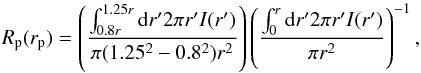 (1)(Blanton et al. 2001; Yasuda et al. 2001) reaches 0.2, in line with the value adopted by the SDSS pipeline. The Petrosian flux (FP) is defined as the flux within Np Petrosian radii. We set N = 2, once again consistently with the SDSS algorithm. For consistency, Petrosian magnitudes are computed in both the g and i images within the same aperture, determined in the white frame.
Similarly, the set of ellipses generated on the white image is used to evaluate both the g and i surface brightness profiles. Both are computed down to the Σsky surface brightness limit, see the example shown in Fig. 3.
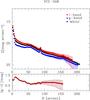 |
Fig. 3 Surface brightness profiles of the Virgo galaxy VCC-508. The g, i and white profiles are respectively show in blue, red and black in the top panel. All are traced down to Σsky. In the bottom panel, the color profile is plotted. |
Finally, the (g−i) color image is obtained performing the operation  , where Img and Imi are respectively the g and i sky-subtracted image and Im(g−i) is the color image. The color profile, truncated where the rms ~ 1σsky;(g−i), is obtained subtracting the i- from the g-band surface brightness profile.
3.3. Errors
In order to evaluate errors on the surface brightness profiles, we take into account the Poissonian statistical noise ( , where S are the counts) and the noise contributed by the statistics of the background, which has units of flux per area (i.e., surface brightness). This corresponds to the total observed individual pixel background σ integrated over the area A. Nevertheless, the MONTAGE software resamples the images of multiple SDSS fields building a mosaicked image of the target object with a generalized drizzle algorithm. The draw-backs are a Moirè pattern (Cotini et al. 2013), a slight image degradation (Blanton et al. 2011) and a mild correlation in the noise of pixels which can lead to an underestimate of the statistic of background. The Moiré pattern is in general non relevant (Cotini et al. 2013) and the degradation of the image is indeed very small (Blanton et al. 2011). Hence, following standard procedures (e.g., Gawiser et al. 2006 and Fumagalli et al. 2014), we estimated the correlated noise that possibly affects our sky noise determination, especially within wide apertures. We compute an empirical noise model for the images, by measuring the flux standard deviation in aperture of npix pixels within sky regions empty of sources, according to the segmentation map. We fit the size-dependent standard deviation with the function
  (2)where σ1 is the individual pixel standard deviation and α and β are the best-fit parameters that typically have a value of α ~ 1 and β ~ 0.56 within our sample (where β = 0.5 means uncorrelated noise), implying a small but non-zero correlation in the pixel noise. The sky errors are therefore evaluated following the fitted function. Finally we consider an additional important source of error that comes from residual gradient of the flat field, which is estimated to be 10% of the rms in the individual pixel by Gavazzi (1993). This represents the dominant source of error in the low surface brightness regions and must therefore be taken into account. The total noise (N) is therefore estimated to be the quadratic sum of the empirical noise model, sky (corrected for the noise correlation) and flat fielding errors:
  (3)where C are the counts, G the gain of the CCD, ΔA is the annuli area and A is the area of the aperture.
The magnitudes into the aperture are  (4)Errors on magnitudes in the profile can therefore be written as:
  (5)where S is the observed flux and N is the noise. In the (g−i) color profiles, the noise (N(g−i)) is computed as the quadratic sum of the Ng and Ni which are the noise computed with Eq. (3) respectively in g- and i-band.
4. Results
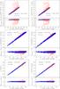 |
Fig. 4 The g-band and i-band Petrosian magnitudes from this work compared to: magnitudes from the SDSS Data Release 10 (Ahn et al. 2014, top panels), those published in Gavazzi et al. (2012, 2013, middle panels), and from the Extended Virgo Cluster Catalog (Kim et al. 2014, bottom panels). Blue points refer to the data within 3σ from the one to one correlation, while the orange points highlight the outliers i.e., galaxies with Δmag > 3σ to the one-to-one relation (where sigma is the standard deviation of the residual distribution). In each panel we report the sigma of the residual distribution as well as the percentage of outliers. We stress that the agreement with Gavazzi et al. (2012, 2013b), Kim et al. (2014) is satisfactory, in particular for the brightest objects (42), that are totally missing in the SDSS DR10. For each plot, the bottom panel reports the residual magnitudes between the two measurements. |
For the 5532 galaxies analyzed with our procedure, we compute g and i Petrosian magnitudes, surface brightness profiles and (g−i) color profiles truncated at 1σ of the background. Petrosian AB magnitudes and colors are given in Table 1 and are available via the online database GOLDMine (Gavazzi et al. 2003, 2014b).
4.1. Magnitudes
In the top panel of Fig. 4, the Petrosian magnitudes extracted with the procedure described above are compared to those downloaded from the data release 10 of the SDSS (Ahn et al. 2014). We found values for 5465 objects, while 383 (~7%) objects are missing in the DR10: 274 are from the local supercluster and 113 from the Coma supercluster. Although a considerable fraction show an appreciable agreement (residuals have a σ ~ 0.13 in both the g- and i-band and median value of −0.05; ~90% of the data is in agreement within 0.4 mag, i.e. 3σ), about 20% of the SDSS magnitudes differs of more than 0.3 mag from our determinations and about 2% of the plotted magnitudes show up to 8 mag discrepancy in the SDSS DR10 database values.
One problem can be ascribed to the SDSS determination of the local background, i.e. by cutting all pixels above a certain sigma level and considering all remaining ones as being part of the background. For large, diffuse, extended objects this leads to a wrong local background determination that is used by the pipeline. The distribution of the residuals (bottom diagram of the top panels of Fig. 4) saturates at faint magnitudes indicating a systematic effect in small and low surface brightness systems (5th percentile at ~−0.75 while the 95th percentile falls at ~0.05). We checked in the photometric catalog of the DR10 for possible causes of such an effect and found that the most deviant points are indeed low surface brightness, blue systems that are flagged as NOPETRO by the SDSS pipeline. This means that their Petrosian radius could not be measured by the pipeline in the r-band (because of their low S/N, Lupton et al. 2001; Strauss et al. 2002) and it is set to the PSF FWHM, thus deriving PSF magnitudes for objects which are indeed extended. The other (less extreme) deviant points are again irregularly shaped, blue galaxies all reporting photometric flags indicating problems either with the raw data, the image or the evaluation of the Petrosian quantities (Lupton et al. 2001; Strauss et al. 2002) such as: DEBLENDED_AS_PSF (deblending problems), DEBLEND_NOPEAK, MANYPETRO3, etc. In these cases, the SDSS pipeline underestimates the Petrosian radius and hence the aperture for the photometry. Henceforth we stress that our procedure is not affected by this problem because it measures the Petrosian radius in the white image which has an improved S/N. This allows us to derive reliable magnitudes even in low surface brightness systems and, in general, systematically measure a larger Petrosian radius (hence Petrosian flux) if compared to the SDSS r-band Petrosian radius. Nevertheless we stress that, the fact that the Petrosian flux is taken within two Petrosian radii ensures that both apertures gather substantially the same Petrosian flux for the vast majority of the sample (Graham & Driver 2005), i.e., the total flux. Moreover, DR10 lacks almost completely the brightest and most extended galaxies (g ≲ 11, i ≲ 10), as demonstrated by the distribution of the 383 objects that are not included in the SDSS database shown in Fig. 5.
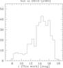 |
Fig. 5 Distribution of magnitudes that are missing in the SDSS catalog as a function of the i-band apparent magnitude from this work. |
In fact, considering both discrepant and missing magnitudes, ~9% of the SDSS data are either unreliable or missing. In particular, in the local supercluster, the percentage of missed galaxies of the DR10 is around 26% and, if we consider objects below 11 mag, it reaches a dramatic 95%, reflecting the difficulties of the SDSS pipeline when dealing with nearby extended objects. Moreover, the few (12) bright galaxies (g < 11 mag) included in the DR10 deviates more than 3σ from the one-to-one correlation in Fig. 4. On the other hand, in the Coma supercluster, the percentage of missing and unreliable galaxies drops to 3% thanks to the smaller angular size of the objects.
To overcome the above discrepancies, about 400 galaxies of the local supercluster have been manually measured using IRAF/QPHOT by Gavazzi et al. (2012). Moreover, for nearly 5000 galaxies in the Coma Supercluster the magnitudes were derived from the SDSS DR7 by Gavazzi et al. (2013b). We compare our automatically extracted magnitudes with those from Gavazzi et al. (2012, 2013b) (which are publicly available via the online database GOLDMine, Gavazzi et al. 2013c, 2014b) obtaining a satisfactory agreement (median difference of ~−0.025 mag), as shown in Fig. 4 (middle panels), especially below 11 mag. At the faint end there is less agreement, as ~15% of galaxies show a residual between the two measurements that exceeds 0.3 mag. The 5th percentile of the residuals distribution is ~−0.45 mag while the 95th percentiles is ~0.2 mag, indicating that the systematic effect at low surface brightness affecting the DR10, affects the Gavazzi et al. measurements too. In fact, despite Gavazzi et al. checked the reliability of the magnitudes taken from the SDSS database of the magnitudes of the DR7, these were not re-calculated and therefore suffer similar problems as the DR10 data. As a matter of fact, the most discrepant objects are once again mainly blue and low surface brightness and are flagged in the SDSS photometry as problematic data. Hence, we believe that the observed discrepancies are again to be attributed to a bad evaluation of the Petrosian radius by the SDSS pipeline among some irregular and low surface brightness systems.
More recently, Kim et al. (2014) released the new Extended Virgo Cluster Catalog (EVCC) which covers an area 5.2 times larger than that of the VCC catalog (Binggeli et al. 1985). It includes 676 galaxies that were not included in the original VCC catalog. Similarly to our work, the EVCC is based on SDSS DR7 images, but it includes all the five SDSS bands ugriz determined using Source Extractor with parameters that are tailored by inspection of the individual galaxies.
We found 844 galaxies in common with the EVCC and we compared their g and i magnitudes with our results. The resulting correlation is plotted in Fig. 4 (bottom panels) and shows a more than satisfactory agreement (median residual of −0.009 mag, σ ~ 0.07) between the two measurements. In particular, we remark the good agreement reached below 14 mag indicating that, unlike the SDSS photometric pipeline, neither the shredding problem nor the aperture radius measurement affect the results of both semi-automated methods. Moreover, 85% of the galaxies differs by less than 0.2 mag between the two studies. The Kim et al. (2014) magnitudes are measured by Source Extractor within an aperture with radius equal to k times the Kron radius (Graham & Driver 2005) of the galaxy, where k is the Kron factor and is set to k = 2.5. This value is chosen because is expected to recover more than 94% of the total flux (Bertin & Arnouts 1996). Therefore the agreement further demonstrate that the aperture radius set to two times the Petrosian radius evaluated in the white image recovers efficiently the total flux of the galaxy. Despite the overall excellent agreement, 6% of galaxies above mag ~15 display a difference between our and their measurements that exceeds 0.3 mag (~5 × σ) and, in two cases, the two determinations differs of ~3 mag. The vast majority of these discrepant objects appear significantly fainter in our analysis and are low surface brightness systems that lie very near to bright sources (e.g., stars, interacting galaxies etc.). We re-measured these magnitudes with IRAF/QPHOT and concluded that some contaminating light has likely not been fully masked by Kim et al. (2014).
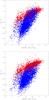 |
Fig. 6 Top: color magnitude diagram of the observed colors displaying the well known bimodal distribution for late type galaxies (blue cloud, blue dots) and early type galaxies (red sequence, red dots). Bottom: the color magnitude diagram after the inclination correction has been applied. The red sequence and the blue cloud are well separated at all masses. |
5. The color−magnitude
After computing the observed magnitudes as described in the previous sections, we correct them for Galactic extinction, following the 100 micron based reddening map of Schlegel et al. (1998), re-calibrated by Schlafly & Finkbeiner (2011). Furthermore, colors of late-type galaxies are corrected for internal extinction using the empirical transformation (Gavazzi et al. 2013b) ![Mathematical equation: \begin{equation} (g-i)_{0}=(g-i)_{\rm mw}-0.17\left(\left[1-\cos(incl)\right]\left[\log\left(\frac{M_{\star}}{{M_{\odot}}}\right)-8.17\right]\right), \end{equation}](/articles/aa/full_html/2016/07/aa27618-15/aa27618-15-eq111.png) (6)where (g−i)mw is the color corrected for Milky Way Galactic extinction, M⋆ is the mass computed with Eq. (7) using the uncorrected color and incl is the inclination of the galaxy, computed following Solanes et al. (1996).
(6)where (g−i)mw is the color corrected for Milky Way Galactic extinction, M⋆ is the mass computed with Eq. (7) using the uncorrected color and incl is the inclination of the galaxy, computed following Solanes et al. (1996).
Stellar masses are derived from the i magnitudes and the inclination corrected color (g−i)0, assuming a Chabrier IMF via the mass vs i-band luminosity relation 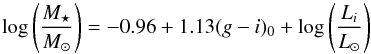 (7)published by Zibetti et al. (2009), where Li is the i-band luminosity of the galaxy in solar units.
Figure 6 (top panel) shows the observed color-mass diagram of the local and Coma superclusters before the inclination correction is applied. The sharp oblique density contrast occurring around 108 M⊙ is caused by the SDSS selection (r< 17.7) at the different distances of the local and Coma superclusters (respectively ~17 Mpc ad ~95 Mpc) and by the mild dependence on galaxy color of the mass-luminosity relation. The local supercluster is indeed less populated due to the lack of sampled volume and is undersampled at high masses. Nevertheless, owing to its proximity, the SDSS selection allows us to include in the analysis galaxies down to masses as low as ~106.5 M⊙. On the contrary, the selection restricts the Coma color-magnitude relation to ≳108.5 M⊙ making the blue cloud relation appear steeper than the local one (see Table 1).
Slopes of the linear fits (g−i) = a + b × lg(M∗) of the blue cloud and red sequence for the local supercluster (Lsc), the Coma supercluster (Csc), the whole sample (All).
Early-type galaxies (dE,dS0, E, S0 and S0a; red dots) form the red sequence while late-type galaxies (from Sa to Irr, blue dots) follow the blue cloud that overlaps with the red sequence at high masses, as highlighted with early SDSS data by Strateva et al. (2001), Hogg et al. (2004). The morphological cut is based on the morphological classification available in GOLDMine (Gavazzi et al. 2003, 2014b). After the internal extinction correction is applied, as in Fig. 6 (Bottom panel), the color magnitude preserves its bimodality, with less overlap at high masses. At this point a note of caution is required: the selection bias that affects the more populated Coma sample prevents us from reliably extract a general slope. Therefore we constraint our fit to the deeper data of the local Universe and find that the slope of the blue cloud remains steeper than that of the red sequence even after the corrections. As a matter of fact, the local blue cloud best fit changes from (g−i)LTG = 0.18 × log (M∗)−0.87 in the uncorrected plot to  (8)when the correction is applied, where (g−i)LTG and (g−i)LTG;0 are respectively the blue cloud uncorrected and corrected color and the error over the slope is as low as ~3 × 10⁻³ in both relations. As expected, since no inclination correction acts on ETGs, the red sequence fit remains consistent in both relations: (g−i)ETG = 0.13 × log (M∗)−0.12.
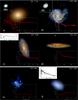 |
Fig. 7 RGB SDSS images and (g−i) extracted color profiles of six galaxies belonging to the local supercluster sample: a) VCC 1154 is an S0 galaxy with a circumnuclear dusty disk of ~800 pc as shown by an archival HST image. The presence of these structures is easily spotted by a clear deviation towards the red on circumnuclear scale in the (g−i) profile at 3′′ as indicated by the vertical white line. b) The barred spiral galaxy VCC 508. Its circumnuclear star-forming disk (highlighted in the inset) produces a deviation towards blue in the color profile at ~10′′ as indicated by the vertical white line. c) VCC-1690 (Boselli et al. 2016), spiral galaxy with a strong blue AGN nuclear (g−i) color. Its nuclear spectra (shown in the inset) exhibit the key signatures of Post StarBurst (PSB) galaxies. d) Late-type galaxy VCC-873. The AGN activity is strongly obscured by dust and its color profile reaches extreme values. e) Irregular galaxy VCC 664 and its blue, nearly flat color profile. f) The low mass galaxy together with its PSB-like nuclear spectrum. Its central emission strongly deviates towards bluer colors with respect of the outermost region of the galaxy. |
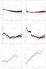 |
Fig. 8 Comparison of our color profiles (red dots) with the ones derived from McDonald et al. (2011; black dots) for six galaxies matching the two samples of different types. From top left to right we plot VCC 1632, VCC 2095, VCC 596, that are respectively an E,S0,Sc (from NED). In the second row we plot VCC 1555, VCC 1356, 1499, respectively an Sc an Sm and a dE. There is an overall good agreement but the profiles display some differences especially in late type galaxies. We ascribe these effects to the difference in the isophotal fitting technique and the one adopted in this work to extract the profiles. McDonald et al. (2011) are indeed sensitive to twists of the isophotes occurring in the presence of spiral arms, bars and even in bright HII regions in irregular galaxies. |
6. Radial color profiles
For each object of the sample, our procedure yields a radial color profile. In this section, we discuss the color profiles extracted by taking a closer look to some prototypical cases. Then we describe more quantitatively the general properties of color profiles along the Hubble sequence creating a set of radial color profile templates of different morphological classes in different mass bins.
In general, the color is a good tracer of the specific SFR: regions actively forming stars have bluer colors than regions of quenched SFR and profile shapes generally correlate with the Hubble type. Early type galaxies (e.g., Es and S0s) typically have almost flat and red profiles, common among the red and dead objects (Tamura & Ohta 2003; Wu et al. 2005). Differently from the ETGs, irregular galaxies are characterized by an almost flat blue profile reflecting their lack of dust and their ongoing SF activity at all radii (Fig. 7, bottom row). Finally spiral galaxies have a composite profile that is blue at large radii and becomes redder only toward the center in correspondence with structures such as bulges or bars (e.g., VCC-1690 in Fig. 7, see also Gavazzi et al. 2015, for a detailed discussion), consistent with the conclusion drawn by Fossati et al. (2013) who compared the distribution of the star formation from Hα imaging flux with the stellar continuum.
Strong deviations from the typical color profiles can be induced by strong dust absorption, as in the case of the highly inclined galaxy VCC-873 shown in Fig. 7. The strongest deviations are observable in the nuclear regions of galaxies, where, for example, nuclear dusty disks are detectable as clear deviations toward a redder color (see, e.g., VCC-1154 in Fig. 7, top-left). On the other hand, unobscured HII regions, dominated by young stars, can cause strong deviations towards the blue in the color profiles. The barred spiral galaxy VCC-508 (Fig. 7, top-right) is the perfect posterchild of this class of objects, with a color profile deviating towards the blue on a scale of 3 arcsec (~300 pc), in correspondence with a star-forming ring (vividly shown in the HST archival image), and possibly in correspondence of the bar Inner Lindblad Resonance (ILR, Kormendy & Kennicutt 2004; Comerón et al. 2010; Font et al. 2014). Similar nuclear blue spikes can be associated to unobscured AGNs and Post StarBurst (PSB) nuclei. An example of galaxy hosting a PSB nucleus is VCC-1499 (shown in Fig. 7), a member of the dEs of the Virgo cluster that display blue nuclei (Lisker et al. 2006). To better test the good quality of our profiles in Fig. 8 we show the comparison between color profiles extracted in this work with the ones derived from the surface brightness profiles published by McDonald et al. (2011) for six galaxies of different morphological types: VCC1632 (E), VCC 2095 (S0), VCC0596 (Sc). VCC1555(Sc), VCC1356(Sm), VCC1499(dE). The agreement is good indicating once again the good quality of the photometry produced by our automatic pipeline. Nevertheless small differences appear especially in late type galaxies in Fig. 8. We ascribe these effects to the fact that the profiles of McDonald et al. (2011) were extracted with an isophotal fitting procedure (i.e., ellipticity and PA of the ellipses are allowed to vary) contrary to ours. In fact the greatest deviations are displayed in VCC0596. VCC1555, VCC1356 that are three late type galaxies, respectively an Sc, Sc and Sm. In these objects, isophotes twists in correspondence with non axisymmetric structures.
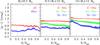 |
Fig. 9 Template color profiles in different bins of mass and morphology. Left panel: low mass bin (M ≤ 108.5 M⊙) where red stands for dwarf ellipticals (dE) and blue for dwarf irregulars (dIrr). Central panel: intermediate mass bin (108.5 M⊙<M ≤ 1010 M⊙) where red dots are for the ETGs (from E to S0a) template, green dots for Spirals (from Sa to Sbc) and blue dots for Sc−Irr LTGs. Right panel: high mass bin (M> 1010 M⊙) where the color code is the same as the intermediate mass bin. In both the high-mass and the intermediate-mass bins, we did not take into account galaxies with incl> 60°. |
6.1. Templates
This section is devoted to a more quantitative analysis of the color profiles and of their correlations with stellar mass and morphology, focusing only on local supercluster galaxies, which are resolved on scales of ~100 pc. Moreover, in this way, we are not affected by the selection bias discussed in Sect. 2. Template profiles allow us to investigate the average properties of color profiles in our sample as a function of mass and morphology. After normalizing each profile to the Petrosian radius and correcting for Galactic extinction, we create template profiles in different bins of stellar mass and morphology with a radial step of 0.05 R/Rpet. Further on we correct the profiles for internal extinction. Despite the fact that we cannot obtain radial extinction profiles, Holwerda et al. (2005) show that on average the radial extinction profiles of spirals are flat within the given errors, except for the very central region (R ≲ 0.2 R25) where extinction can be significantly more severe with respect to the external parts. It is impossible to correct for dust extinction this region relying solely on the optical data and to implement a precise galaxy-to-galaxy dust correction for the whole sample is way beyond the scope of the present study. Therefore we correct the profiles applying the average correction evaluated for the total color of the galaxy. In addition, we did not include galaxies with incl> 60°, in order to avoid contaminations from edge-on spirals whose internal and external colors are dramatically reddened by the dust extinction through the disk plane (see Fig. 7d). We defined three equally populated mass bins:
-
a low mass bin containing galaxies withM∗ ≤ 108.5 M⊙;
-
an intermediate mass bin, in which 108.5<M∗ ≤ 1010 M⊙;
-
a high mass bin, in which 1010<M∗ ≤ 1012 M⊙.
In the intermediate and high mass bins we identified three morphological classes: the first class contains elliptical galaxies, S0s and S0a; the second bin includes late type galaxies from Sa to Sbc while the last bin Sc and irregulars. The cut is based on the morphological classification taken from GOLDMine (Gavazzi et al. 2003, 2014b) which, in the local Universe, is mainly based on the morphological classification performed by de Vaucouleurs et al. (1991) and Binggeli et al. (1985) on photographic plates of exquisite quality.
Galaxies with masses lower than 108.5 M⊙ are either classified as dwarf ellipticals or dwarf irregulars. The resulting template profiles are shown in Fig. 9, separately for each morphological bin.
Summarizing, early type galaxies do not show significant gradients, irrespective of their mass. Late type galaxies show instead flat profiles in the low mass bin while, at higher masses, their profiles show evident color gradients, implying the presence of a red component in their central region whose importance increases with mass. Focusing on the highest mass bin, spirals are as red as ellipticals in their central parts and as blue as dIrrs in their outskirts. In other words, given the well known color-sSFR relation, spirals are primarily quenched in a central region whose importance is a function of mass while their outermost regions remain star forming (Fossati et al. 2013).
7. Color−magnitude decomposition
Inspecting Fig. 9 with the aim of further investigating properties of color gradients, we identified three non-overlapping zones of interest of the color profiles:
-
the nuclear (or innermost) region going from the center of thegalaxy up to approximately1 kpc;
-
an intermediate region defined by 0.2RPet ≤ R ≤ 0.3RPet;
-
an outer, disk-dominated, zone with R ≥ 0.35 RPet.
Figure 10 shows the galaxy color as a function of the total stellar mass for each of the three zones, all corrected for Galactic extinction, with the disk-dominated zone also corrected for inclination. Overall, galaxies belonging to the red sequence are insensitive to this decomposition and show a consistent gradient in all three mass-color diagrams traced by each zone. Instead late-type galaxies populate a blue cloud that show three different distributions for each of the three zone analyzed. While the outer region of late type galaxies follows a relation almost parallel to the red sequence, the inner zones lie on much steeper color-mass relations.
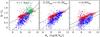 |
Fig. 10 Color−magnitude diagram of three different zones where red dots are ETGs and blue dots are LTGs: (left panel) inner zone, where open green dots are galaxies hosting an active galactic nucleus of different kinds (LINERs, Seyfert, AGN) classified on the basis of nuclear emission lines; (central panel) intermediate zone; right panel: outer, disk-dominated zone. |
7.1. Nuclei
In the left panel of Fig. 10 we plot the color mass diagram of the inner kpc of galaxies in our local supercluster sample. Early type galaxies form a well defined red sequence while late type galaxies lie on the blue cloud. Comparing this diagram to the classical color-magnitude, the red sequence slopes are consistent. Nevertheless, considering nuclear colors, late type galaxies scatter around a much steeper relation that crosses the red sequence at about 109 M⊙, displaying color indices even greater than those for typical early types at M∗> 109.5−10 M⊙. Furthermore, in the mass range 109−1012 M⊙, we highlight galaxies with ongoing nuclear activity, such as AGNs, LINERS and Seyfert (green dots in the left panel in Fig. 10). The adopted nuclear activity classification is based on the ratio of nuclear Hα and [NII] emission lines according to the WHAN (Cid Fernandes et al. 2011) diagram. Nuclear emission lines were taken from the SDSS spectroscopic database Data Release 12 (Alam et al. 2015), complemented with spectra available in NED and other measured by Gavazzi et al. (2013c). Overall we find the nuclear classifications for 91% of the galaxies.
As it can be seen in Fig. 10, these objects, highlighted in green, deviate from the relations followed by the red sequence and the blue cloud and reach the most extreme red values of color indices at any given mass.
To further investigate how the color inside the nuclear region is linked to its nuclear activity we define an index of “central/nuclear reddening”:  (9)where (g−i)nuc is the nuclear-scale color corrected for Galactic extinction and (g−i)0 is the mean color of the galaxy. Qred estimates the deviation of the nuclear color from the average color of the galaxy. Figure 11 shows the distribution of Qred for four different categories of nuclear activity: in orange, we plot the distribution of the RETIRED (galaxies that stopped their star formation and have their gas ionized by old stellar populations, Stasińska et al. 2015) and Passive nuclei galaxies; in red are displayed LINERs, AGNs and Seyfert; blue represents Post StarBurst (PSB) galaxies and green is for HII region-like nuclei.
The identified categories distribute quite differently: Passive and Retired galaxies show a quite tight distribution peaked at Qred ~ 0; Active Galactic Nuclei are undoubtedly associated with colors that are redder than the average of the galaxy. The vast majority (~91%) have values of Qred> 0.0 and only 9% of AGNs display a bluer nucleus with respect to the galaxy color. Moreover, if we consider galaxies reaching the more extreme deviations, i.e. Qred> 0.3, they represent the 45% of the AGNs population. This effect is possibly due to dust absorption associated with the gas fueling the nuclear region, although a contribution from the AGN itself cannot be excluded based only on the optical data. Post Starburst (PSB) galaxies are, on the contrary, associated with nuclei that are bluer with respect to the galaxy color since in 80% of cases PSBs display a Qred< 0; HII-region like nuclei have instead the most widespread distribution of nuclear colors, with respect to the galaxy color. The evidence of a bluer nucleus in PSBs and the fact that they are preferentially found in higher density environments is consistent with a picture where these objects are transitioning from the blue cloud to red sequence quenching their star formation in an outside-in fashion due to a ram pressure stripping event (Gavazzi et al. 2010).
Moreover, if we consider low and high mass galaxies separately (Fig. 11, bottom panel), the distribution is bimodal: HII region-like nuclei in massive galaxies are always redder than the galaxy itself while, at low masses, the distribution is dominated by galaxies showing a nucleus that is bluer with respect to the average color of the galaxy.
This is consistent with a picture where nuclei of small galaxies are more likely to be caught in a bursting act and have little or no dust absorption (Holwerda et al. 2005) while, massive galaxies have on average a redder nucleus with respect to the galaxy color possibly due to dust extinction. Nevertheless, our optical data cannot exclude a contribution from an underlying older stellar population.
7.2. Bulges, bars and disks
Focusing on the second and third panel of Fig. 10, we highlight the intermediate and disk zone contribution to the color−magnitude diagram. The red sequence is once again consistent between the two plots. Indeed, the slopes determined with a least squared fit of the red sequence in the two diagrams are consistently 0.17 ± 0.01 and 0.16 ± 0.01 mag dex-1. On the other hand, the blue cloud differs significantly: its slope varies from 0.34 ± 0.01 mag dex-1 in the innermost region to 0.28 ± 0.01 and 0.18 ± 0.01 mag dex-1 respectively in the intermediate and disk-dominated regions.
Therefore, in the intermediate zone, the blue cloud displays a steep relation although not as steep as in the innermost region. Nevertheless, the blue cloud completely overlaps the red sequence at M∗> 1010 M⊙. This behavior drastically changes in the disk-dominated zone (right panel of Fig. 10). Indeed, the outer-zone color magnitude diagram is composed of two well separated distributions: the blue cloud increases its color with mass following a slope that is almost identical to the red sequence.
In the intermediate zone, above a threshold mass, LTG galaxies have therefore suppressed SF and assume color values typical of ETGs. On the contrary, they mostly appear as normal star forming objects in their outer disks.
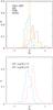 |
Fig. 11 Top: normalized distributions of the nuclear reddening Qr indices for different classes of nuclear activity (computed following Cid Fernandes et al. 2011) color coded as follows: AGNs are represented by a red line; the PSBs distribution is traced by the blu line; the green line stands for HII-like nuclei and the orange for PASSIVE and Retired galaxies. Bottom: normalized distributions of HII-like nuclei above (red) and below (blue) 109 M⊙. |
Moreover, the growth of the red component and the color contamination from the star forming disk (with bluer colors) in this zone can be approximately traced by the color difference between the intermediate and the outer zone shown in Fig. 12, where this difference is plotted as a function of mass. Despite a significant scatter, a Kolmogorov-Smirnov test confirms that the distributions of ETGs and LTGs are not drawn from the same parent sample (P ≲ 10-3). Red and blue lines connect the average difference between the intermediate and outer regions inside bins of 1 log(M∗/M⊙) separately for ETGs (red) and LTGs (blue). This diagram shows that early type galaxies display an average mild gradient of approximately ≲0.1 mag from low to high mass galaxies.
Late type galaxies are instead characterized by a gradient between the two zones whose importance increases with mass. This is consistent with a picture where galaxies develop a red and dead, quenched structure in their central regions, the relevance of which depends on mass. In their disks, instead, late type galaxies preserve their star formation almost unaffected. Nevertheless, even the outer regions, which are occupied by SF structures and are therefore blue, still display an increasingly red color with increasing mass (see Fig. 10, right panel). As a note of caution, we remind that the correction for internal extinction is not radially dependent and although it is a good approximation, some small residual contribution of the dust absorption might still affect the profiles. Nevertheless, visual inspection of many images and profiles support the idea that the main cause of the red color observed is due to different stellar populations instead of dust extinction.
8. Discussion
Our method successfully led to a set of final optical color-based parameters that trace some properties of nuclei, bulges, and disks among our local sample. In our analysis, we searched for systematic gradients in (g−i) color profiles in different galaxy types. Here we compare our results with literature studies and discuss their implications for galaxy formation and evolution.
We investigated color gradients with two different techniques: in Sect. 6.1 we built color profiles templates for different morphological classes in three bins of increasing mass; in Sect. 7 we relate the galaxy total stellar mass versus the average color of three different, non-overlapping regions in which respectively nuclei, bulges (and/or bars) and disks are the dominant structure. As a general result, regardless of the binning used, colors show a mass dependency, with more massive galaxies harboring redder structures with respect to their lower mass counterparts (see Fig. 10), confirming different literature results.
8.1. Nuclei
Our investigation of nuclear regions confirms the tight correlation existing between the color of nuclei and the luminosity/mass of the host-galaxy that has been consistently observed in detailed studies of massive Virgo cluster galaxies by the ACS Virgo cluster survey (Côté et al. 2006) and of fainter galaxies of the Virgo and Fornax clusters (Lotz et al. 2004). We find that the correlation holds for both faint and bright galaxies although it shows a large scatter in the bright end of the distribution. Consistently, Côté et al. (2006) have shown that the brightest early type galaxies show a considerable scatter in the nuclear color magnitude. Nevertheless, a note of caution is required: the scale that defines our innermost region extends up to 1 kpc, which is approximately ten times the scale length of the nuclei studied in the ACS Virgo cluster survey and by Lotz et al. (2004) both relying on HST data. In particular, we note that our innermost region extends to the typical distance within which dusty structures such as the one in Fig. 3a are found. In the ACS these represents ~20% of the ETGs and therefore at least for these early type galaxies, the high reddening is likely dominated by the presence of structures of dust instead of their underlying stellar populations. Nevertheless we still find evidences of the results drawn by Lotz et al. (2004) and Côté et al. (2006): all nuclear regions of bright ETGs are redder than their harboring galaxy (Côté et al. 2006) while, at the faint end of the red sequence, nuclear colors are more scattered and often bluer than the color of their host galaxy (see top panel of Fig. 12).
LTGs show similar trends although strongly amplified compared to the ETGs. Intriguingly, among the high mass, scattered population of both ETGs and LTGs, it appears to be a correlation between the color in the innermost region and the AGN activity of the nucleus: nuclei of active galaxies are found on average to be redder than their non-active counterparts (see Fig. 10). Nevertheless, given the large extension of our innermost region, we refrain from considering the AGN as main contributors to the color of the nuclei in these galaxies, as such effect could be related to the extinction caused by the dust dragged by the gas that occupies the region and fuels the AGN. Our analysis is consistent with the stellar population study presented by Côté et al. (2006) who find an old/intermediate stellar population component in the nuclear regions of all bright galaxies (ETGs and LTGs). These still follow a color magnitude relation despite the scatter at high mass that suggests that, at least for the most deviant population, the nuclear chemical enrichment was governed by internal/local factors. The presence of disky dusty structures even in evolved systems such as Es and S0s suggests that the region is periodically refurbished with gas and dust. For example, secular disk instabilities or mergers can funnel the gas and the dust toward the very center of the galaxy. Consequently the strong degeneracy between absorption and stellar population age on such scales prevents from a unique interpretation of the history of these structures relying solely on optical data (Driver et al. 2007). Further on, as it is shown in the faint end of the two distributions in Fig 12 (top), many LTGs have nuclei that are bluer compared to the galaxy color (Taylor et al. 2005) and, despite a considerable scatter, many ETGs also display blue nuclei consistently with Lisker et al. (2006). Our spectroscopic analysis revealed that a fraction of the population of blue nuclei is possibly populated by PSB galaxies (see Fig. 11) which have recently experienced a recent, sudden shut down of star formation and by nuclei that retain some residual SF activity (HII-like) despite the poor HI content of the host galaxy. These systems are undergoing an outside-in quenching of the star formation in the Virgo cluster hinting at physical processes such as harassment (Moore et al. 1996) and ram pressure stripping (Gunn & Gott 1972) as possible causes of such evolutionary paths.
8.2. Bulges, bars and disks
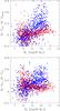 |
Fig. 12 Top: distribution of the difference between the color indexes of the nuclear zone and the color of the galaxy plotted against the total stellar mass. Bottom: distribution of the difference between the color indexes of the intermediate zone and those of the disk-dominated zone plotted against the total stellar mass. In both panels, the blue and red small dots stand for respectively the blue cloud and the red sequence galaxies. The blue (red) line connects the average value in 4 bins of 10log (M/M⊙) from 107 to 1011 M⊙ for LTGs (ETGs). |
Despite the considerable scatter in both colors and color gradients (Peletier & Balcells 1996; Taylor et al. 2005; Roediger et al. 2011a), the tight correlation between color and stellar mass of the host galaxies holds true in both the region identified as intermediate and outer in Sect. 7. ETGs form a tight red sequence (see Fig. 10) for both regions and show an average inside-out gradient of ~0.1 mag (Fig. 12, bottom). LTGs form instead two different distributions: the blue cloud of the intermediate (or bulge/bar) region becomes red (i.e., it reaches the red sequences) above 1010 M⊙ while the outer, disk-dominated region never overlaps completely the red sequence. Still, more massive disks are redder than their lower mass counterparts but the difference between the colors of the outer and the intermediate region increases with respect to the total stellar mass. This can be possibly induced by the growth of a red and dead structure in the center of massive disks, i.e. that the central part of galaxies underwent a star formation quenching process that turned them red. Our results on the average properties of color profiles broadly agree with literature data. For example MacArthur et al. (2004) have shown that the radial profile of the average ages of the stellar populations decreases from inside out and that the steepness of the decrease is a function of morphological type. Color templates shown in Fig. 9 exhibit a radial behavior fully consistent with the average age profiles shown by MacArthur et al. (2004). We find there is also a good agreement with the (g−H) color profiles published in Roediger et al. (2011a) for almost all the morphological types, although in their median profiles of early disks they find positive color gradients (and consistently positive age population gradients in their stellar population analysis, Roediger et al. 2011b) that we do not see. Roediger et al. (2011b) do not find any direct link between galaxy morphologies and the observed stellar population gradients. On the contrary, studies such as Cheung et al. (2013) and Gavazzi et al. (2015) have shown that the bar occupation fraction rises steeply above 109.5 M⊙ (as also confirmed by the works done by Skibba et al. 2012; Masters et al. 2012) and that, above this mass,galaxies are progressively more quenched (red) in their centers, while their disks still sustain SF and hence are blue. These studies therefore highlight that the presence of structures such as bars can indeed produce the color gradients that we observe and likely also the stellar population gradients. These authors thus conclude that a secular bar drives the quenching of the star formation in the central kiloparsecs of galaxies. Moreover massive galaxies undergo bar instability earlier than their lower mass counterparts and thus have more time to grow redder than low mass systems. Moreover, Méndez-Abreu et al. (2012) on a study of the Virgo bar fraction have shown that this rises up to more than 50% above 1010 M⊙, adding a further link between color/stellar populations radial gradients that we observe and structures such as bars (Laurikainen et al. 2010). We stress, however, that disk instabilities can also rejuvinate the central stellar population by, e.g., triggering central star formation in correspondence of the ILRs of spirals or bars (an example could be the one of VCC 508 in Fig. 3a).
Both MacArthur et al. (2004) and Roediger et al. (2011a), also observe a positive gradient in low mass galaxies. Among these galaxies we find only a mild gradient in the template profile of dIrr in Fig. 9. From Fig. 12 we are taken to conclude that positive gradients can be found in low mass galaxies especially if we consider the most internal regions (Lisker et al. 2006; Fossati et al. 2013) in contrast to the external parts but that the severe scattering occurring at low mass in our parameters prevents from extracting a robust general trend. This could be related to the fact that the low mass population may be composed of objects with different formation processes (van Zee et al 2004; Lisker et al. 2008). In our sample, positive gradients are most noticeable in the nuclear region (Fig. 12, top) while in the comparison between the color of the intermediate region with the color of the disk-dominated region their difference is consistent with zero.
9. Summary and Conclusions
In this paper we have presented a semi-automated, IDL-based, procedure designed to perform photometric extraction on SDSS multi-band images. The procedure was used to analyze a magnitude and volume limited sample of 5532 galaxies in the local and Coma superclusters. Our procedure, unlike the SDSS pipeline, avoids the so-called shredding problem and successfully extracts total Petrosian magnitudes even for the largest objects of the sample, recovering 383 g- (and i-) band magnitudes not included in the SDSS DR10 (Ahn et al. 2014). After the galactic and internal extinction correction is applied, we recover a refined color-magnitude diagram of the local and Coma superclusters.
We attempted to dissect the color of galaxies in three distinct contributions: a nuclear region, an intermediate (0.2RPet ≤ R ≤ 0.3RPet), and an external region. To this end, we analyzed the high quality color profiles that our routine has extracted for each galaxy, focusing on the objects of the local supercluster sample, with the best spatial resolution. Our analysis highlighted that: Profiles are powerful tools for the detection of structures on nuclear scales (ILRs, dusty disks etc.) even when they are difficult to be visually spotted on SDSS images.
-
i)
Nuclei of galaxies display the greatest deviations with respect tothe galaxy color. This deviation correlates mildly with the nuclearactivity of the galaxy. Passive galaxies do not deviate from thecolor of the galaxy while AGNs generally display very red nuclearcolors. Star forming nuclei follow instead a bimodal distribution:galaxies that are more massive than 109 M⊙ display redder nuclear color with respect to the galaxy while galaxies with M< 109 M⊙ have bluer nuclei. Overall, a wide population of low mass galaxies display bluer nuclei with respect to their average color see Fig. 12 (top) although the high scatter does not allow the extraction of a general trend.
-
ii
Profiles of spiral galaxies reveal on average an intermediate zone that is redder with respect of the outer disk and this component is more important at high masses.
-
iii
The intermediate zone color of LTGs overlaps the red sequence already at 109 M⊙ and is completely superposed to it at 1010 M⊙ (Figs. 10 and 12).
-
iv
The disks of spiral galaxies follow a distribution that does not overlap (and is almost parallel to) with the red sequence but that still displays an increasing color index with increasing mass.
From i) we conclude that a wide population of low mass galaxies undergo an outside-in quenching of their star formation consistent with an evolution driven by the environment on short timescales (Boselli & Gavazzi 2006; Lisker et al. 2006; Fossati et al. 2013). Nevertheless this conclusion does not hold for the whole population at low mass, as testified by the large scatter in their photometric parameters in both ETGs and LTGs. From ii) and iii) we conclude that massive spiral galaxies develop a red and dead component, the importance of which increases with mass. Moreover, i) and iii) lead us to conclude that this component must arise in a range mass between 109 M⊙ and 1010 M⊙ but that this component is not the only contribution to the slope of the global color-magnitude. In fact, iv) demonstrates that even after subtracting the red and dead component another process (such as strangulation, Peng et al. 2015; Fiacconi et al. 2015) is required to progressively quench the star formation in the outer regions of massive disks.
The procedure is able to process all the SDSS bands images at the same time. Nevertheless, in this paper we present the analysis of only the g- and i-band images. Obviously adding more bands affects the S/N of the white image and therefore the detection performed by Source Extractor.
To speed up the procedure we set the step between adjacent ellipses (along the semi-major axis) as a function of the image dimensions: 1 pixel for images smaller than 300 pixels; 2 pixels for images greater than 300 pixels, up to 1000 pixels; 4 pixels for images greater than 1000 pixels.
In irregular low surface brightness systems there may be more than one Petrosian radius, Lupton et al. (2001).
Acknowledgments
The authors would like to thank the referee, Thorsten Lisker, for his constructive criticism. This research has made use of the GOLDmine database (Gavazzi et al. 2003, 2014b) and of the NASA/IPAC Extragalactic Database (NED) which is operated by the Jet Propulsion Laboratory, California Institute of Technology, under contract with the National Aeronautics and Space Administration. We wish to thank an unknown referee whose criticism helped improving the manuscript. Funding for the Sloan Digital Sky Survey (SDSS) and SDSS-II has been provided by the Alfred P. Sloan Foundation, the Participating Institutions, the National Science Foundation, the US Department of Energy, the National Aeronautics and Space Administration, the Japanese Monbukagakusho, and the Max Planck Society, and the Higher Education Funding Council for England. The SDSS Web site is http://www.sdss.org/. The SDSS is managed by the Astrophysical Research Consortium (ARC) for the Participating Institutions. The Participating Institutions are the American Museum of Natural History, Astrophysical Institute Potsdam, University of Basel, University of Cambridge, Case Western Reserve University, The University of Chicago, Drexel University, Fermilab, the Institute for Advanced Study, the Japan Participation Group, The Johns Hopkins University, the Joint Institute for Nuclear Astrophysics, the Kavli Institute for Particle Astrophysics and Cosmology, the Korean Scientist Group, the Chinese Academy of Sciences (LAMOST), Los Alamos National Laboratory, the Max-Planck-Institute for Astronomy (MPIA), the Max-Planck-Institute for Astrophysics (MPA), New Mexico State University, Ohio State University, University of Pittsburgh, University of Portsmouth, Princeton University, the United States Naval Observatory, and the University of Washington. M. Fossati acknowledges the support of the Deutsche Forschungsgemeinschaft via Project ID 3871/1−1. M. Fumagalli acknowledges support by the Science and Technology Facilities Council [grant number ST/L00075X/1].
References
- Aaronson, M., Persson, S. E., & Frogel, J. A. 1981, ApJ, 245, 18 [NASA ADS] [CrossRef] [Google Scholar]
- Abazajian, K. N., Adelman-McCarthy, J. K., Agüeros, M. A., et al. 2009, ApJS, 182, 543 [NASA ADS] [CrossRef] [Google Scholar]
- Adelman-McCarthy, J. K., Agüeros, M. A., Allam, S. S., et al. 2006, ApJS, 162, 38 [NASA ADS] [CrossRef] [Google Scholar]
- Ahn, C. P., Alexandroff, R., Allen de Prieto, C., et al. 2014, ApJS, 211, 17 [NASA ADS] [CrossRef] [Google Scholar]
- Alam, S., Albareti, F. D., Allen de Prieto, C., et al. 2015, ApJS, 219, 12 [NASA ADS] [CrossRef] [Google Scholar]
- Baldwin, J. A., Phillips, M. M., & Terlevich, R. 1981, PASP, 93, 5 [NASA ADS] [CrossRef] [EDP Sciences] [Google Scholar]
- Baldry, I. K., Glazebrook, K., Brinkmann, J., et al. 2004, ApJ, 600, 681 [NASA ADS] [CrossRef] [Google Scholar]
- Bell, E. F., Wolf, C., Meisenheimer, K., et al. 2004, ApJ, 608, 752 [NASA ADS] [CrossRef] [Google Scholar]
- Berriman, G. B., Good, J. C., Laity, A. C., et al. 2004, Astronomical Data Analysis Software and Systems (ADASS) XIII, 314, 593 [Google Scholar]
- Bertin, E., & Arnouts, S. 1996, A&AS, 117, 393 [NASA ADS] [CrossRef] [EDP Sciences] [Google Scholar]
- Binggeli, B., Sandage, A., & Tammann, G. A. 1985, AJ, 90, 1681 [NASA ADS] [CrossRef] [Google Scholar]
- Blanton, M. R., Dalcanton, J., Eisenstein, D., et al. 2001, AJ, 121, 2358 [NASA ADS] [CrossRef] [Google Scholar]
- Blanton, M. R., Lin, H., Lupton, R. H., et al. 2003, AJ, 125, 2276 [NASA ADS] [CrossRef] [Google Scholar]
- Blanton, M. R., Schlegel, D. J., Strauss, M. A., et al. 2005, AJ, 129, 2562 [NASA ADS] [CrossRef] [Google Scholar]
- Blanton, M. R., Kazin, E., Muna, D., Weaver, B. A., & Price-Whelan, A. 2011, AJ, 142, 31 [NASA ADS] [CrossRef] [Google Scholar]
- Boselli, A., & Gavazzi, G. 2006, PASP, 118, 517 [NASA ADS] [CrossRef] [Google Scholar]
- Boselli, A., Boissier, S., Heinis, S., et al. 2011, A&A, 528, A107 [NASA ADS] [CrossRef] [EDP Sciences] [Google Scholar]
- Boselli, A., Cuillandre, J. C., Fossati, M., et al. 2016, A&A, 587, A68 [NASA ADS] [CrossRef] [EDP Sciences] [Google Scholar]
- Chester, C., & Roberts, M. S. 1964, AJ, 69, 635 [NASA ADS] [CrossRef] [Google Scholar]
- Cheung, E., Athanassoula, E., Masters, K. L., et al. 2013, ApJ, 779, 162 [NASA ADS] [CrossRef] [Google Scholar]
- Cid Fernandes, R., Stasińska, G., Mateus, A., & Vale Asari, N. 2011, MNRAS, 413, 1687 [NASA ADS] [CrossRef] [Google Scholar]
- Comerón, S., Knapen, J. H., Beckman, J. E., et al. 2010, MNRAS, 402, 2462 [NASA ADS] [CrossRef] [Google Scholar]
- Côté, P., Piatek, S., Ferrarese, L., et al. 2006, ApJS, 165, 57 [NASA ADS] [CrossRef] [MathSciNet] [Google Scholar]
- Cotini, S., Ripamonti, E., Caccianiga, A., et al. 2013, MNRAS, 431, 2661 [NASA ADS] [CrossRef] [Google Scholar]
- de Vaucouleurs, G., de Vaucouleurs, A., Corwin, H. G., Jr., et al. 1991, Third Reference Catalogue of Bright Galaxies; Volume I: Explanations and references; Volume II: Data for galaxies between 0h and 12h; Volume III: Data for galaxies between 12h and 24h, eds. G. de Vaucouleurs, A. de Vaucouleurs, H. G. Corwin, Jr., et al. (New York, NY: Springer, USA) [Google Scholar]
- Driver, S. P., Popescu, C. C., Tuffs, R. J., et al. 2007, MNRAS, 379, 1022 [NASA ADS] [CrossRef] [Google Scholar]
- Faber, S. M. 1973, ApJ, 179, 731 [NASA ADS] [CrossRef] [Google Scholar]
- Fiacconi, D., Feldmann, R., & Mayer, L. 2015, MNRAS, 446, 1957 [NASA ADS] [CrossRef] [Google Scholar]
- Font, J., Beckman, J. E., Querejeta, M., et al. 2014, ApJS, 210, 2 [NASA ADS] [CrossRef] [Google Scholar]
- Fossati, M., Gavazzi, G., Savorgnan, G., et al. 2013, A&A, 553, A91 [NASA ADS] [CrossRef] [EDP Sciences] [Google Scholar]
- Fumagalli, M., O’Meara, J. M., Prochaska, J. X., Kanekar, N., & Wolfe, A. M. 2014, MNRAS, 444, 1282 [NASA ADS] [CrossRef] [Google Scholar]
- Gavazzi, G. 1993, ApJ, 419, 469 [NASA ADS] [CrossRef] [Google Scholar]
- Gavazzi, G. 2009, Rev. Mex. Astron. Astrofis. Conf. Ser., 37, 72 [NASA ADS] [Google Scholar]
- Gavazzi, G., Pierini, D., & Boselli, A. 1996, A&A, 312, 397 [NASA ADS] [Google Scholar]
- Gavazzi, G., Boselli, A., Scodeggio, M., Pierini, D., & Belsole, E. 1999, MNRAS, 304, 595 [NASA ADS] [CrossRef] [Google Scholar]
- Gavazzi, G., Boselli, A., Donati, A., Franzetti, P., & Scodeggio, M. 2003, A&A, 400, 451 [NASA ADS] [CrossRef] [EDP Sciences] [Google Scholar]
- Gavazzi, G., Giovanelli, R., Haynes, M. P., et al. 2008, A&A, 482, 43 [NASA ADS] [CrossRef] [EDP Sciences] [Google Scholar]
- Gavazzi, G., Fumagalli, M., Cucciati, O., & Boselli, A. 2010, A&A, 517, A73 [NASA ADS] [CrossRef] [EDP Sciences] [Google Scholar]
- Gavazzi, G., Fumagalli, M., Galardo, V., et al. 2012, A&A, 545, A16 [NASA ADS] [CrossRef] [EDP Sciences] [Google Scholar]
- Gavazzi, G., Fumagalli, M., Galardo, V., et al. 2013a, A&A, 553, A89 [NASA ADS] [CrossRef] [EDP Sciences] [Google Scholar]
- Gavazzi, G., Savorgnan, G., Fossati, M., et al. 2013b, A&A, 553, A90 (Paper III) [NASA ADS] [CrossRef] [EDP Sciences] [Google Scholar]
- Gavazzi, G., Consolandi, G., Dotti, M., et al. 2013c, A&A, 558, A68 [NASA ADS] [CrossRef] [EDP Sciences] [Google Scholar]
- Gavazzi, G., Franzetti, P., & Boselli, A. 2014b, ArXiv e-prints [arXiv:1401.8123] [Google Scholar]
- Gavazzi, G., Consolandi, G., Dotti, M., et al. 2015, A&A, 580, A116 [NASA ADS] [CrossRef] [EDP Sciences] [Google Scholar]
- Gawiser, E., van Dokkum, P. G., Herrera, D., et al. 2006, ApJS, 162, 1 [NASA ADS] [CrossRef] [Google Scholar]
- Graham, A. W., & Driver, S. P. 2005, PASA, 22, 118 [NASA ADS] [CrossRef] [Google Scholar]
- Griersmith, D. 1980, AJ, 85, 1135 [NASA ADS] [CrossRef] [Google Scholar]
- Gunn, J. E., & Gott, J. R., III 1972, ApJ, 176, 1 [NASA ADS] [CrossRef] [Google Scholar]
- Haynes, M. P., Giovanelli, R., Martin, A. M., et al. 2011, AJ, 142, 170 [NASA ADS] [CrossRef] [Google Scholar]
- Hogg, D. W., Blanton, M. R., Brinchmann, J., et al. 2004, ApJ, 601, L29 [NASA ADS] [CrossRef] [Google Scholar]
- Holwerda, B. W., Gonzalez, R. A., Allen, R. J., & van der Kruit, P. C. 2005, AJ, 129, 1396 [NASA ADS] [CrossRef] [Google Scholar]
- Katz, D. S., Berriman, G. B., & Mann, R. G. 2011, in Reshaping Research and Development Using Web 2.0-based Technologies, ed. M. Baker (Nova Science Publishers, Inc.) [Google Scholar]
- Kauffmann, G., White, S. D. M., Heckman, T. M., et al. 2004, MNRAS, 353, 713 [NASA ADS] [CrossRef] [Google Scholar]
- Kim, S., Rey, S.-C., Jerjen, H., et al. 2014, ApJS, 215, 22 [Google Scholar]
- Kormendy, J., & Kennicutt, R. C., Jr. 2004, ARA&A, 42, 603 [NASA ADS] [CrossRef] [Google Scholar]
- Landsman, W. B. 1993, Astronomical Data Analysis Software and Systems II, ASP Conf. Ser., 52, 246 [NASA ADS] [Google Scholar]
- Laurikainen, E., Salo, H., Buta, R., Knapen, J. H., & Comerón, S. 2010, MNRAS, 405, 1089 [NASA ADS] [Google Scholar]
- Lisker, T., Glatt, K., Westera, P., & Grebel, E. K. 2006, AJ, 132, 2432 [NASA ADS] [CrossRef] [Google Scholar]
- Lisker, T., Grebel, E. K., & Binggeli, B. 2008, AJ, 135, 380 [NASA ADS] [CrossRef] [Google Scholar]
- Lotz, J. M., Miller, B. W., & Ferguson, H. C. 2004, ApJ, 613, 262 [NASA ADS] [CrossRef] [MathSciNet] [Google Scholar]
- Lupton, R., Gunn, J. E., Ivezić, Z., Knapp, G. R., & Kent, S. 2001, Astronomical Data Analysis Software and Systems X, ASP Conf. Ser., 238, 269 [NASA ADS] [Google Scholar]
- MacArthur, L. A., Courteau, S., Bell, E., & Holtzman, J. A. 2004, ApJS, 152, 175 [NASA ADS] [CrossRef] [Google Scholar]
- Masters, K. L., Nichol, R. C., Haynes, M. P., et al. 2012, MNRAS, 424, 2180 [NASA ADS] [CrossRef] [Google Scholar]
- McDonald, M., Courteau, S., Tully, R. B., & Roediger, J. 2011, MNRAS, 414, 2055 [NASA ADS] [CrossRef] [Google Scholar]
- Mei, S., Blakeslee, J. P., Côté, P., et al. 2007, ApJ, 655, 144 [NASA ADS] [CrossRef] [Google Scholar]
- Melvin, T., Masters, K., Lintott, C., et al. 2014, MNRAS, 438, 2882 [NASA ADS] [CrossRef] [Google Scholar]
- Méndez-Abreu, J., Sánchez-Janssen, R., Aguerri, J. A. L., Corsini, E. M., & Zarattini, S. 2012, ApJ, 761, L6 [NASA ADS] [CrossRef] [Google Scholar]
- Micheva, G., Östlin, G., Bergvall, N., et al. 2013, MNRAS, 431, 102 [NASA ADS] [CrossRef] [Google Scholar]
- Moore, B., Katz, N., Lake, G., Dressler, A., & Oemler, A. 1996, Nature, 379, 613 [NASA ADS] [CrossRef] [Google Scholar]
- Nair, P. B., & Abraham, R. G. 2010, ApJ, 714, L260 [NASA ADS] [CrossRef] [Google Scholar]
- Peletier, R. F., & Balcells, M. 1996, AJ, 111, 2238 [NASA ADS] [CrossRef] [Google Scholar]
- Peng, Y., Maiolino, R., & Cochrane, R. 2015, Nature, 521, 192 [NASA ADS] [CrossRef] [Google Scholar]
- Roediger, J. C., Courteau, S., McDonald, M., & MacArthur, L. A. 2011a, MNRAS, 416, 1983 [NASA ADS] [CrossRef] [Google Scholar]
- Roediger, J. C., Courteau, S., MacArthur, L. A., & McDonald, M. 2011b, MNRAS, 416, 1996 [NASA ADS] [CrossRef] [Google Scholar]
- Solanes, J. M., Giovanelli, R., & Haynes, M. P. 1996, ApJ, 461, 609 [NASA ADS] [CrossRef] [Google Scholar]
- Schlegel, D. J., Finkbeiner, D. P., & Davis, M. 1998, ApJ, 500, 525 [NASA ADS] [CrossRef] [Google Scholar]
- Schlafly, E. F., & Finkbeiner, D. P. 2011, ApJ, 737, 103 [NASA ADS] [CrossRef] [Google Scholar]
- Skibba, R. A., Masters, K. L., Nichol, R. C., et al. 2012, MNRAS, 423, 1485 [NASA ADS] [CrossRef] [Google Scholar]
- Stasińska, G., Costa-Duarte, M. V., Vale Asari, N., Cid Fernandes, R., & Sodré, L. 2015, MNRAS, 449, 559 [NASA ADS] [CrossRef] [Google Scholar]
- Strateva, I., Ivezić, Ž., Knapp, G. R., et al. 2001, AJ, 122, 1861 [Google Scholar]
- Strauss, M. A., Weinberg, D. H., Lupton, R. H., et al. 2002, AJ, 124, 1810 [NASA ADS] [CrossRef] [Google Scholar]
- Tamura, N., & Ohta, K. 2003, AJ, 126, 596 [NASA ADS] [CrossRef] [Google Scholar]
- Taylor, V. A., Jansen, R. A., Windhorst, R. A., Odewahn, S. C., & Hibbard, J. E. 2005, ApJ, 630, 784 [NASA ADS] [CrossRef] [Google Scholar]
- van Zee, L., Barton, E. J., & Skillman, E. D. 2004, AJ, 128, 2797 [NASA ADS] [CrossRef] [Google Scholar]
- Visvanathan, N., & Griersmith, D. 1977, A&A, 59, 317 [NASA ADS] [Google Scholar]
- Visvanathan, N., & Sandage, A. 1977, ApJ, 216, 214 [NASA ADS] [CrossRef] [Google Scholar]
- Wu, H., Shao, Z., Mo, H. J., Xia, X., & Deng, Z. 2005, ApJ, 622, 244 [NASA ADS] [CrossRef] [Google Scholar]
- Xue, Y. Q., Brandt, W. N., Luo, B., et al. 2010, ApJ, 720, 368 [NASA ADS] [CrossRef] [Google Scholar]
- Yasuda, N., Fukugita, M., Narayanan, V. K., et al. 2001, AJ, 122, 1104 [NASA ADS] [CrossRef] [Google Scholar]
- York, D. G., Adelman, J., Anderson, J. E., Jr., et al. 2000, AJ, 120, 1579 [Google Scholar]
- Zibetti, S., Charlot, S., & Rix, H.-W. 2009, MNRAS, 400, 1181 [NASA ADS] [CrossRef] [Google Scholar]
- Zwicky, F., Herzog, E., & Wild, P. 1968, A Catalogue of Galaxies and Clusters of Galaxies (Pasadena: California Institute of Technology – CIT) [Google Scholar]
Appendix A: Source Extractor setup
Source Extractor (version 2.5.0) remains one of the central tools of the procedure. It has the crucial task to create the best possible mask for the field of view, crucial to obtain a robust sky estimate, and to evaluate the geometrical parameters of the target, fundamental to create the proper set of ellipses (Sect. 3.2). This is performed in the higher signal to noise white image (see Sect. 3.1). The most challenging task is to guide Source Extractor to find efficiently small as well as large galaxies and properly de-blend bright contaminating sources minimizing the light loss from the target.
As our sample is dominated by galaxies belonging to the Coma supercluster, spanning a range of apparent dimensions from few tens of arc-seconds to few arc-minutes, we chose to favor a setup that works well with galaxies of this size and we implement an ad-hoc procedure (described in Appendix B) for the few larger galaxies (all belonging to the local supercluster), that extend for ~10 arcmin and contain many resolved substructures.
For all other galaxies, we list here the best set of initial Source Extractor options that we adopted for the analysis. In order to obtain a segmentation map for each image analyzed the CHECKIMAGE_TYPE parameter must be turned on SEGMENTATION. Parameters that regulate the minimum number of pixel and the minimum flux limit for a detection are DETECT_MINAREA and DETECT_THRESH which we set respectively to 5 pixels and 1.5 sigmas (THRESH_TYPE = RELATIVE). This parameters are the best to account for faint galaxies and galaxies affected by bright sources as also confirmed by Kim et al. (2014). For all galaxies, the deblending parameters we adopted are DEBLEND_MINCONT = 0.001 and DEBLEND_NTHRESH = 16. Further on, we modified the memory parameter MEMORY_PIXSTACK bringing it to 300 000. Moreover, as we are only interested in the geometry of the target (PA, axis ratio and best pixel center coordinates), we did not accurately tune parameters regulating the photometric extraction and the best sky estimate of Source Extractor.
Appendix B: Dealing with large nearby galaxies
Although our procedure is able to analyze galaxies that span a wide range of apparent dimensions, the Source Extractor setup we adopted (Appendix A) fails for 3% of the largest galaxies of the sample, all belonging to the local supercluster. In fact, galaxies belonging to the local supercluster have many resolved substructures e.g., perturbed spiral arms, strongly obscuring dust lanes, bright HII regions etc.
These structures sometimes reach the deblending parameters (see Appendix A) according to which Source Extractor separates overlapping objects. Therefore some substructures of the galaxy are detected by Source Extractor as entities not belonging to the target.
As a consequence, the area of the galaxy in the segmentation map is not composed by a single patch but, instead, by as many patches as the different structures deblended by Source Extractor.
As described in Sect. 3.1, our procedure exploits the segmentation map in order to produce the mask for the image by removing the central patch assuming that this is the only mask (of a galaxy, parameter CLASS_STAR ~ 0) (Sect. 3.1). Therefore, in the case of the 3% of problematic galaxies, our procedure would remove only a part of the mask covering the area occupied by the galaxy, leading to a wrong magnitude. To avoid the problem, the user must provide a list of the biggest galaxies, listing the following parameters:
-
RA in degrees;
-
Dec in degrees;
-
A, the major axis of the galaxy in arcmin;
-
B, the minor axis of the galaxy in arcmin;
-
PA, the position angle in degrees.
These parameters, taking advantage of the WCS system, are used to define the area occupied by the target galaxy as the pixels inside the ellipse
![Mathematical equation: \appendix \setcounter{section}{2} \begin{eqnarray} &&x=a \cos(\phi)\cos({\rm PA})-b \sin(\phi)\sin({\rm PA}) \\[3mm] &&y=a \cos(\phi)\sin({\rm PA})+b \sin(\phi)\cos({\rm PA}), \end{eqnarray}](/articles/aa/full_html/2016/07/aa27618-15/aa27618-15-eq207.png) where PA is the position angle, a and b respectively the semi-major and semi-minor axis and φ the azimuthal angle going from 0 to 2π. Within this area, the procedure removes all masks but the one that have been assigned by Source Extractor the CLASS_STAR parameter exceeding 0.8.
where PA is the position angle, a and b respectively the semi-major and semi-minor axis and φ the azimuthal angle going from 0 to 2π. Within this area, the procedure removes all masks but the one that have been assigned by Source Extractor the CLASS_STAR parameter exceeding 0.8.
Magnitudes extracted and corrected (g−i) colors of the whole sample (one page sample).
All Tables
Slopes of the linear fits (g−i) = a + b × lg(M∗) of the blue cloud and red sequence for the local supercluster (Lsc), the Coma supercluster (Csc), the whole sample (All).
Magnitudes extracted and corrected (g−i) colors of the whole sample (one page sample).
All Figures
|
Fig. 1 Sky projection (top) and Wedge diagram (bottom) of galaxies belonging to the sample studied in this work: the Coma supercluster (δ> 18°; cz> 4000 km s-1) and the local supercluster (δ< 18°; cz< 3000 km s-1). Blue dots represent late type galaxies (LTGs) while red dots stand for early type galaxies (ETGs). The dotted rectangular regions indicate the areas surveyed by ALFALFA. |
| In the text | |
|
Fig. 2 Sky surface brightness distributions in g- (blue line) and i-band (red line) for the sample analyzed in this work. The vertical dashed lines indicate the mean surface brightness in g- and i-band respectively ⟨ Σi ⟩ = 24.36 ± 0.16 and ⟨ Σg ⟩ = 25.43 ± 0.17 mag arcsec-2. |
| In the text | |
|
Fig. 3 Surface brightness profiles of the Virgo galaxy VCC-508. The g, i and white profiles are respectively show in blue, red and black in the top panel. All are traced down to Σsky. In the bottom panel, the color profile is plotted. |
| In the text | |
|
Fig. 4 The g-band and i-band Petrosian magnitudes from this work compared to: magnitudes from the SDSS Data Release 10 (Ahn et al. 2014, top panels), those published in Gavazzi et al. (2012, 2013, middle panels), and from the Extended Virgo Cluster Catalog (Kim et al. 2014, bottom panels). Blue points refer to the data within 3σ from the one to one correlation, while the orange points highlight the outliers i.e., galaxies with Δmag > 3σ to the one-to-one relation (where sigma is the standard deviation of the residual distribution). In each panel we report the sigma of the residual distribution as well as the percentage of outliers. We stress that the agreement with Gavazzi et al. (2012, 2013b), Kim et al. (2014) is satisfactory, in particular for the brightest objects (42), that are totally missing in the SDSS DR10. For each plot, the bottom panel reports the residual magnitudes between the two measurements. |
| In the text | |
|
Fig. 5 Distribution of magnitudes that are missing in the SDSS catalog as a function of the i-band apparent magnitude from this work. |
| In the text | |
|
Fig. 6 Top: color magnitude diagram of the observed colors displaying the well known bimodal distribution for late type galaxies (blue cloud, blue dots) and early type galaxies (red sequence, red dots). Bottom: the color magnitude diagram after the inclination correction has been applied. The red sequence and the blue cloud are well separated at all masses. |
| In the text | |
|
Fig. 7 RGB SDSS images and (g−i) extracted color profiles of six galaxies belonging to the local supercluster sample: a) VCC 1154 is an S0 galaxy with a circumnuclear dusty disk of ~800 pc as shown by an archival HST image. The presence of these structures is easily spotted by a clear deviation towards the red on circumnuclear scale in the (g−i) profile at 3′′ as indicated by the vertical white line. b) The barred spiral galaxy VCC 508. Its circumnuclear star-forming disk (highlighted in the inset) produces a deviation towards blue in the color profile at ~10′′ as indicated by the vertical white line. c) VCC-1690 (Boselli et al. 2016), spiral galaxy with a strong blue AGN nuclear (g−i) color. Its nuclear spectra (shown in the inset) exhibit the key signatures of Post StarBurst (PSB) galaxies. d) Late-type galaxy VCC-873. The AGN activity is strongly obscured by dust and its color profile reaches extreme values. e) Irregular galaxy VCC 664 and its blue, nearly flat color profile. f) The low mass galaxy together with its PSB-like nuclear spectrum. Its central emission strongly deviates towards bluer colors with respect of the outermost region of the galaxy. |
| In the text | |
|
Fig. 8 Comparison of our color profiles (red dots) with the ones derived from McDonald et al. (2011; black dots) for six galaxies matching the two samples of different types. From top left to right we plot VCC 1632, VCC 2095, VCC 596, that are respectively an E,S0,Sc (from NED). In the second row we plot VCC 1555, VCC 1356, 1499, respectively an Sc an Sm and a dE. There is an overall good agreement but the profiles display some differences especially in late type galaxies. We ascribe these effects to the difference in the isophotal fitting technique and the one adopted in this work to extract the profiles. McDonald et al. (2011) are indeed sensitive to twists of the isophotes occurring in the presence of spiral arms, bars and even in bright HII regions in irregular galaxies. |
| In the text | |
|
Fig. 9 Template color profiles in different bins of mass and morphology. Left panel: low mass bin (M ≤ 108.5 M⊙) where red stands for dwarf ellipticals (dE) and blue for dwarf irregulars (dIrr). Central panel: intermediate mass bin (108.5 M⊙<M ≤ 1010 M⊙) where red dots are for the ETGs (from E to S0a) template, green dots for Spirals (from Sa to Sbc) and blue dots for Sc−Irr LTGs. Right panel: high mass bin (M> 1010 M⊙) where the color code is the same as the intermediate mass bin. In both the high-mass and the intermediate-mass bins, we did not take into account galaxies with incl> 60°. |
| In the text | |
|
Fig. 10 Color−magnitude diagram of three different zones where red dots are ETGs and blue dots are LTGs: (left panel) inner zone, where open green dots are galaxies hosting an active galactic nucleus of different kinds (LINERs, Seyfert, AGN) classified on the basis of nuclear emission lines; (central panel) intermediate zone; right panel: outer, disk-dominated zone. |
| In the text | |
|
Fig. 11 Top: normalized distributions of the nuclear reddening Qr indices for different classes of nuclear activity (computed following Cid Fernandes et al. 2011) color coded as follows: AGNs are represented by a red line; the PSBs distribution is traced by the blu line; the green line stands for HII-like nuclei and the orange for PASSIVE and Retired galaxies. Bottom: normalized distributions of HII-like nuclei above (red) and below (blue) 109 M⊙. |
| In the text | |
|
Fig. 12 Top: distribution of the difference between the color indexes of the nuclear zone and the color of the galaxy plotted against the total stellar mass. Bottom: distribution of the difference between the color indexes of the intermediate zone and those of the disk-dominated zone plotted against the total stellar mass. In both panels, the blue and red small dots stand for respectively the blue cloud and the red sequence galaxies. The blue (red) line connects the average value in 4 bins of 10log (M/M⊙) from 107 to 1011 M⊙ for LTGs (ETGs). |
| In the text | |
Current usage metrics show cumulative count of Article Views (full-text article views including HTML views, PDF and ePub downloads, according to the available data) and Abstracts Views on Vision4Press platform.
Data correspond to usage on the plateform after 2015. The current usage metrics is available 48-96 hours after online publication and is updated daily on week days.
Initial download of the metrics may take a while.