© ESO, 2016

1. Introduction

Continuum radio galaxy surveys can probe large cosmic volumes. The mean redshift of observed radio galaxies is significantly higher than the mean redshift of modern optical surveys. Optical surveys allow us to obtain photometric or even spectroscopic redshift measurements, which is not the case for continuum radio galaxy surveys. Nevertheless, the information contained in continuum radio galaxy surveys can be useful for probing cosmological models. An example is the investigation of non-Gaussianity via angular two-point correlations. In this work we revisit some aspects of the cosmological analysis of continuum radio galaxy surveys.

Most of our current understanding of cosmology relies on observations of the cosmic microwave background (CMB). Planck satellite data extended our understanding to the high multipole CMB, and allowed us to successfully measure the cross-correlation between the large-scale structure and the CMB through the integrated Sachs-Wolfe (ISW) and lensing effects. In the study of the ISW effect, large-scale radio continuum catalogues play an important role. For the Planck analysis the NRAO VLA Sky Survey (NVSS; Condon et al. 1998) has been utilized (Planck Collaboration XIX 2014).

Radio galaxy surveys, such as the NVSS, have large sky coverage and extend to redshifts well beyond unity. Their angular two-point correlation function and angular power spectrum are useful probes of large-scale cosmology. With new radio continuum surveys, containing between 10 million to a few billion objects, such as from the Low Frequency Array (LOFAR)¹, the Australian Square Kilometre Array Pathfinder (ASKAP)², the South African MeerKAT radio telescope (MeerKAT)³ or the Square Kilometre Array (SKA)⁴, more complete and precise radio point source catalogues will be available. These surveys will allow us to probe several interesting aspects of cosmology (for a recent review see Jarvis et al. 2015), including accurate investigations of the largest cosmic structures.

For cosmological analysis the fundamental observable from a survey is the surface density of sources above a given flux density limit, i.e. the integral of the differential number count per solid angle per flux density interval as a function of position on the sky. A study that includes all effects of the surface density at linear order in cosmological perturbation theory has been presented recently (Maartens et al. 2013; Chen & Schwarz 2015). These effects could be modified by local effects of large structures, e.g. by local voids (Rubart et al. 2014). Radio continuum surveys are also a good candidate to further test several CMB anomalies (Bennett et al. 2011; Copi et al. 2010, 2015a,b; Naselsky et al. 2012; Planck Collaboration XXIII 2014; Planck Collaboration XVI 2016).

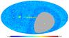Fig. 1 Surface density of the NVSS source catalogue in galactic coordinates in Mollweide projection, shown at healpix resolution Nside = 32. The colour bar shows the surface density in units of number of objects per square degree. Here we include all objects contained in the catalogue. The white dots indicate the the positions of the celestial poles.

Previously, Blake & Wall (2002b) explored the angular two-point correlation of the NVSS catalogue at small angular separation (θ< 10°). In addition, they also measured the angular power spectrum of the same catalogue (Blake et al. 2004), and found that their result seems to be incompatible with a high redshift population of radio galaxies. Xia et al. (2010) suggested that the clustering at 1° ≤ θ ≤ 8° is dominated by some non-Gaussian component. They quote the non-Gaussianity parameter 25 <f_nl< 117 at 2σ. The angular power spectrum was also tested more recently in Marcos-Caballero et al. (2013), which also find an excess of power at large scales, but −43 <f_nl< 142 at 2σ. Hernández-Monteagudo (2010) investigated in detail the two-point cross-correlation between the NVSS catalogue and the CMB temperature anisotropies from the Wilkinson Microwave Anisotropy Probe (WMAP) in angular and multipole space. He did not find any evidence for the cross-correlation in the range l ∈ [2,10] where, according to the simulation 50% of the signal is expected. He concluded that the large-scale clustering excess, which he found in the NVSS catalogue, is unlikely to be caused by contaminants or systematics since it appears to be independent of the flux density threshold.

In this work, we explore the full range of the angular two-point correlation function (0°<θ< 180°) with a focus on large angular scales (≥1°) and compare it with the flat Λ cold dark matter (ΛCDM) model. The focus of our investigation lies on how to prepare a catalogue from a real all-sky radio continuum survey for cosmological analysis, rather than the estimation of cosmological parameters. All previous analyses are based on masking of the galaxy by a constant latitude cut. Moreover the cosmic radio dipole (Ellis & Baldwin 1984; Blake & Wall 2002a) has not been accounted for in previous works. To extract the auto-correlation signal from the catalogue in a reliable way, we propose a more sophisticated NVSS mask and subtract the cosmic radio dipole. Based on sidelobe contamination estimates and noise properties of the NVSS catalogue, we provide a mask that leaves us with a sky coverage of 64.7% at a minimal specific flux density of 15 mJy.

Our work is structured as follows. In Sect. 2 we review the properties of the NVSS catalogue and explain our masking method. In Sect. 3, we review the theoretical angular two-point correlation function based on the ΛCDM model. We present the angular two-point correlation obtained by means of the Landy-Szalay estimator using our mask in Sect. 4. In Sect. 5 we discuss our results, followed by the conclusion in Sect. 6.

2. NVSS catalogue

The NRAO VLA Sky Survey Condon et al. (1998) used the D and DnC antenna configurations of the Very Large Array (VLA). The survey was carried out between 1993 and 1997. Continuum intensity and linear polarization images at 1.4 GHz were obtained, covering the whole northern and part of the southern sky at declinations δ> −40°. The D configuration of the VLA was used to cover the sky from δ = −10° to δ = 78°, the rest was filled in by means of the DnC configuration. The obtained images have on average a FWHM resolution θ_FWHM = 45′′, which is significantly larger than the median angular size of faint extragalactic sources (around 10′′). This survey design sacrifices resolution to achieve high surface brightness, which is needed to achieve flux-limit completeness.

Since the NVSS point-source response is much larger than the median angular size of extragalactic sources, most of the information on the NVSS total intensity images is represented well by elliptical Gaussian fits. The fitted parameters formed the NVSS catalogue of sources (not all of which are individual sources). The NVSS catalogue contains almost 2 million discrete sources with flux density above 2.5 mJy. Below we use the source positions in right ascension α and declination δ, the integrated flux density S, and their errors.

The NVSS catalogue contains several artificial effects (Ho et al. 2008): First, the catalogue shows a configuration effect, which is easily seen in Fig. 1 as steps in surface density at δ ~ 78° and δ ~ −10°, which are the borders between the D and DnC configurations on the map. Second, the sidelobes of the bright sources can obscure the presence of weak nearby sources. They are not completely removed by cleaning. The NVSS local dynamic range of the total intensity images is about 1000 to 1. Thus, sources closer than about 0.6° to a bright source of flux density S and fainter than 10^-3S can only be caused by sidelobes (Condon et al. 1998).

In addition to these two unphysical effects, there is also a foreground of point sources mainly from the Milky Way (see Fig. 1) and smooth components of radiation from the galaxy itself. These contaminations can influence the VLA noise temperature, and further change the completeness in certain areas on the sky.

All these effects need to be treated carefully, otherwise the statistical analysis based on the contaminated map will be biased. Here we choose to apply a lower flux density threshold and to mask the catalogue to address these issues.

2.1. Lower flux density threshold

Two different VLA configurations (D and DnC) have been used to compile the NVSS catalogue. The VLA C configuration is less compact and has a resolution of 15′′, which is better than 45′′ of the D configuration. The DnC configuration is a hybrid configuration in which the antennas on the east and west arms are in D configuration, but those on the north arm are in C configuration to enhance their view of sources at low elevation. Using the DnC configuration changes the synthesized beam and the resolution of declination with respect to the D configuration. This shifts the brightness sensitivity and completeness between the parts of sky observed with different configurations.

The source catalogue is derived from intensity images, therefore it is brightness sensitivity limited. Apparently, the D configuration has higher brightness sensitivity than the DnC configuration. Thus a more complete catalogue for the part of the sky observed by means of the D configuration is expected.

The completeness shift of the DnC configuration sky with respect to the D configuration sky can be considered as a faint source selection based on the position angle, noise, confusion and cataloguing procedures. It is not clear whether this selection also introduces a tension in source distribution between the two parts of the sky. Therefore, it is safe to either use one configuration alone (which would reduce the sky coverage by a significant amount), or to choose a higher flux density threshold for the cosmological analysis (which reduces the source density and increases the shot noise).

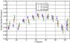Fig. 2 Surface density fluctuation, $\mathrm{\Delta }\mathit{\sigma }\mathit{/}\overline{\mathit{\sigma }}$, of the NVSS catalogue as a function of declination for several flux density thresholds. The error bars assume Poisson distributed source counts and we mask the region | b | ≤ 5°. For clarity, the horizontal positions of the S> 5 mJy and S> 15 mJy data points are slightly offset.

Blake & Wall (2002b) argue that this configuration effect is only significant at flux densities S< 10 mJy. In Fig. 2 we plot the surface density fluctuation, $\mathrm{\Delta }\mathit{\sigma }\mathit{/}\overline{\mathit{\sigma }}\mathrm{=}\mathit{\sigma }\mathit{/}\overline{\mathit{\sigma }}\mathrm{-}\mathrm{1}$, as a function of declination. The dependence of the surface density fluctuation on declination resembles the theoretical rms noise level of the NVSS catalogue (Condon et al. 1998), which is discussed further in Sect. 5. It can be seen that the declination dependence of the surface density is less than 2.5% and the mean value of the DnC configuration is clearly lower than that of the D configuration. This configuration effect is more pronounced at lower thresholds.

This finding is also supported by a χ²-analysis testing for deviations from isotropy in declination ${\mathit{\chi }}^{\mathrm{2}}\mathrm{\equiv }\sum _{\mathit{i}\mathrm{=}\mathrm{1}}^{{\mathit{N}}_{\mathrm{bin}}}\frac{{\mathrm{(}{\frac{\mathrm{\Delta }{\mathit{\sigma }}_{\mathit{i}}}{\mathit{\sigma ̅}}}^{\mathrm{)}}}^{\mathrm{2}}}{{\left(\mathit{\delta }{\mathrm{[}{\frac{\mathrm{\Delta }\mathit{\sigma }}{\mathit{\sigma ̅}}}^{\mathrm{]}}}_{\mathit{i}}\right)}^{\mathrm{2}}}\mathrm{=}\sum _{\mathit{i}\mathrm{=}\mathrm{1}}^{{\mathit{N}}_{\mathrm{bin}}}{\mathrm{\Omega }}_{\mathit{i}}\frac{{\left(\mathrm{\Delta }{\mathit{\sigma }}_{\mathit{i}}\right)}^{\mathrm{2}}}{{\mathit{\sigma }}_{\mathit{i}}}\mathit{,}$(1)where Ω_i denotes the solid angle of the ith declination strip. The results of this test are shown in Table 1.

In this work, we choose flux density thresholds of 15 mJy and 25 mJy for cosmological analysis for the following reasons: The study of the configuration effect suggests that there is a significant dependence on declination. As is shown above, a flux density threshold of 15 mJy or 25 mJy reduces the value of χ² dramatically compared to the situation with lower thresholds. As we do not expect a perfect agreement with isotropy, it is not justified to raise the threshold even higher.

Our choice is supported by studies of the cosmic radio dipole from NVSS, which is one to two orders of magnitudes larger than the higher multipole moments. The previous NVSS dipole measurements show that for thresholds below 15 mJy, the dipole direction differs significantly from the CMB dipole direction, and the reduced χ² of the quadratic dipole estimator increases significantly (Blake & Wall 2002a; Gibelyou & Huterer 2012; Rubart & Schwarz 2013; Rubart 2015).

No cut-off at high flux densities is introduced as there is only a small number of sources at high flux densities and thus they only play a subdominant role. We also expect them to be less affected by calibration systematics.

2.2. Masking strategy

Nevertheless, we have to mask regions around the brightest sources in order to minimize contamination from their sidelobes. In the analysis of Ho et al. (2008) all sources above 2.5 Jy have been masked by a disk with a radius of 0.6°. However, not all sidelobes appear as spurious entries in the catalogue, a uniform masking strategy will erase all the information from bright sources, since all sources above the cut threshold are masked. In Blake & Wall (2002b) a list of 22 masks around bright galaxies was compiled based on a visual inspection of the survey.

Here, we introduce an automatic bright source selection method. We count the number of nearby sources (within 0.6°) with S> 15 mJy of the brightest sources whose flux densities are S> 2.5 Jy. The corresponding histogram is shown in Fig. 3.

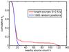Fig. 3 Cumulative distribution of nearby source counts (disks with radius 0.6°). The red line corresponds to nearby source counts around bright radio galaxies with S> 2.5 Jy. The blue line corresponds to 1000 randomly picked positions outside the galactic plane (| b | > 5°). The maximum of randomly picked counts results in 49 nearby sources.

We assume that the number of sources in a fixed solid angle follows a Poisson distribution, and use the so-called Poissonness plot (Hoaglin & Tukey 2006) to identify the histogram bins that significantly deviate from a Poisson distribution, where we assume that such a deviation is caused by the sidelobe contamination of bright sources. The idea of the plot is to consider a simple variable substitution, which transforms the exponential Poisson distribution function to a linear function. We find that 49 sources fail the Poissonness test at the 99% confidence level (Fig. 4). It is worth clarifying that “clean” regions containing bright sources that, by chance, contain the same amount of sources as “dirty” regions are also excluded. We also verify that for most of the bright sources the cumulative nearby source distribution is in good agreement with the cumulative distribution of randomly picked nearby source counts, which justifies the inclusion of many of the bright sources in our analysis.

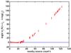Fig. 4 Poissonness plot of the nearby source counts. λo is the mean nearby count over the survey area. N is the total number of sources with S> 2.5 Jy. The solid horizontal line corresponds to a perfectly Possion distributed nearby source count. The error bars denote the 99% confidence levels.

We now turn to the issue of noise and confusion. According to Condon et al. (1998), the rms position uncertainty σ_pos is ${\mathit{\sigma }}_{\mathrm{pos}}\mathrm{\propto }\frac{{\mathit{\sigma }}_{\mathrm{b}}{\mathit{\theta }}_{\mathrm{FWHM}}}{\mathrm{2}{\mathit{S}}_{\mathrm{p}}}\mathit{,}$(2)where S_p is the peak flux density and σ_b is the rms brightness fluctuation (noise and confusion). Our idea is to use σ_pos to trace σ_b. Condon et al. (1998) point out that for flux densities below 15 mJy, the rms position uncertainty is dominated by noise. Accordingly, we create a position uncertainty map (Fig. 5) by averaging the position uncertainties ${\mathit{\sigma }}_{\mathit{\theta }}\mathrm{\equiv }\sqrt{\frac{{\mathit{\sigma }}_{\mathit{\delta }}{\mathit{\sigma }}_{\mathit{\alpha }}}{{\mathit{\theta }}_{\mathrm{FWHM}}^{\mathrm{2}}}\sin \left(\frac{\mathit{\pi }}{\mathrm{2}}\mathrm{-}\mathit{\delta }\right)}$(3)for all point sources in a pixel whose flux density is smaller than 15 mJy. We note that the dominant sources are those with low flux density. The map is constructed using the healpix package with the pixel size fixed by Nside = 32.

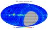Fig. 5 NVSS position uncertainty map, relative to the mean beam width θFWHM = 45′′.

The resulting position uncertainty map is shown in Fig. 5. Which clearly shows that the position uncertainty follows the theoretical rms noise level which, outside of the galactic plane, increases away from the zenith owing to pickup of ground radiation, atmospheric emission, ionospheric effects and uv-projection. The galactic plane and nearby nebulas are also easy to identify. We also employ a 5% pixel cutoff for the pixels with highest σ_θ> 0.132. In addition, we mask galactic radio sources by excluding all sources with galactic latitude | b | ≤ 5°.

To sum up, at 15 mJy and 25 mJy thresholds we mask all pixels in the neighbourhood of 49 selected bright sources. Additional pixels and their neighborhood with highest mean position uncertainty σ_Ω and galactic sources with | b | ≤ 5° are masked as well. In the following we call this the NVSS65 mask⁵. It is shown in Fig. 6. In total, approximately 64.7% of the sky is left. The total number of objects after applying the NVSS65 mask at 15 and 25 mJy is shown in Table 3.

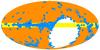Fig. 6 NVSS65 mask. The orange region makes up 64.7% of the sky. Yellow pixels are close to the galactic plane | b | ≤ 5° and are excluded to suppress galactic point sources and foregrounds. Blue pixels are excluded owing to large position errors. Red and black pixels contain bright sources with significant sidelobe effects; black pixels also overlap with pixels with high position error.

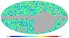Fig. 7 Surface density of the NVSS source catalogue for a flux density threshold of S> 15 mJy and applying the NVSS65 mask, shown in galactic coordinates at pixel size Nside=32. The colour bar shows the surface density σ in units of number of objects per square degree.

3. Angular two-point correlation: theoretical expectation

The angular two-point correlation function w(θ) is a powerful tool for measuring the projected large-scale structure distribution of the Universe. It is defined as the joint probability δP of finding galaxies in both of the elements of solid angle δΩ₁ and δΩ₂ separated by an angle θ (Peebles 1980), $\mathit{\delta P}\mathrm{=}\mathit{\sigma ̅}\mathrm{2}\mathit{\delta }{\mathrm{\Omega }}_{\mathrm{1}}\mathit{\delta }{\mathrm{\Omega }}_{\mathrm{2}}\mathrm{[}\mathrm{1}\mathrm{+}\mathit{w}\mathrm{(}\mathit{\theta }\mathrm{\left)}\mathrm{\right]}\mathit{.}$(4)At linear order, the full relativistic expression of the surface density of sources above flux density S_t is (Chen & Schwarz 2015), $\begin{array}{ccc}\mathit{\sigma }\mathrm{\left(}\mathit{>}{\mathit{S}}_{\mathit{t}}\mathrm{\right)}& \mathrm{=}& \int \begin{array}{c}\mathrm{\infty }\\ {\mathit{S}}_{\mathit{t}}\end{array}\frac{\mathrm{d}{\mathit{S}}_{\mathrm{o}}}{{\mathit{S}}_{\mathrm{o}}}\frac{{\mathit{a}}^{\mathrm{3}}{\mathit{r}}_{\mathrm{o}}^{\mathrm{3}}\mathit{n̅}\mathrm{phy}}{\mathrm{2}\mathrm{+}\mathrm{(}\mathit{\alpha ̅}\mathrm{+}\mathrm{1}\mathrm{)}{\mathit{r}}_{\mathrm{o}}\mathrm{\mathscr{H}}}[\mathrm{1}\mathrm{+}{\mathit{\delta }}_{\mathit{n}}\mathrm{+}\mathrm{3}\mathit{\psi }\mathrm{+}\mathrm{\Delta }\mathit{E}\\ & & \mathrm{+}{\mathit{V}}^{\mathrm{\prime }\mathit{i}}{\mathit{e}}_{\mathit{i}}^{\mathit{r}}\mathrm{+}\mathrm{2}\frac{\mathit{\delta r}}{{\mathit{r}}_{\mathrm{o}}}\mathrm{+}\frac{\mathit{\partial \delta r}}{\mathit{\partial }{\mathit{r}}_{\mathrm{o}}}\mathrm{-}\mathrm{2}{\mathit{\kappa }}_{\mathrm{g}}]\mathit{,}\end{array}$(5)where S_o is the observed flux density, a is the scale factor, r_o is the inferred comoving distance, is the mean source spectrum index, ℋ is the conformal Hubble parameter, and is the physical mean number density. Inside the brackets, the most important contribution comes from the number density fluctuation δ_n. The other terms describe volume distortion via the scalar metric perturbations ψ and E; light cone projection involving the projected source velocity ${\mathit{V}}^{\mathrm{\prime }\mathit{i}}{\mathit{e}}_{\mathit{i}}^{\mathit{r}}$; radial distance fluctuation 2δr/r_o + ∂δr/∂r_o, which lead to a fluctuations of flux density; and lensing convergence κ_g. We only take the dominant leading term, i.e. physical number density fluctuation, into account and neglect all other effects. This is justified since the statistical and systematic fluctuations from the NVSS catalogue are well above the expected size of the subleading linear effects.

The luminosity and density evolution of radio galaxies is significant. Therefore, we turn to redshift space, $\begin{array}{ccc}\mathit{\sigma }\mathrm{(}\mathit{>}{\mathit{S}}_{\mathit{t}}\mathrm{)}& \mathrm{\approx }& \mathit{c}\mathrm{\int }\mathrm{d}\mathit{z}\frac{{\mathit{a}}^{\mathrm{3}}{\mathit{r}}_{\mathrm{o}}^{\mathrm{2}}}{\mathit{H}}\mathit{n̅}\mathrm{phy}\mathrm{[}\mathrm{1}\mathrm{+}{\mathit{\delta }}_{\mathit{n}}\mathrm{]}\\ & \mathrm{=}& \mathrm{\int }\mathrm{d}\mathit{z}\frac{\mathrm{d}\mathit{\sigma ̅}}{\mathrm{d}\mathit{z}}\mathrm{[}\mathrm{1}\mathrm{+}\mathit{b\delta }\mathrm{]}\mathit{,}\end{array}$(6)where b = b(z) denotes the bias of radio galaxies and δ is the matter density contrast in synchronous comoving coordinates.

We use the Combined EIS-NVSS Survey Of Radio Sources (CENSORS; Brookes et al. 2008) to model the redshift distribution of the NVSS catalogue. CENSORS contains all the NVSS sources above 7.2 mJy that are within a patch of 6 deg² in the ESO Imaging Survey (EIS). Following Marcos-Caballero et al. (2013), we choose the gamma function redshift distribution, 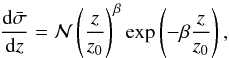$\frac{\mathrm{d}\mathit{\sigma ̅}}{\mathrm{d}\mathit{z}}\mathrm{=}\mathrm{𝒩}{\left(\frac{\mathit{z}}{{\mathit{z}}_{\mathrm{0}}}\right)}^{\mathit{\beta }}\exp \left(\mathrm{-}\mathit{\beta }\frac{\mathit{z}}{{\mathit{z}}_{\mathrm{0}}}\right)\mathit{,}$(7)with denoting a normalization factor that is irrelevant for the final result and the best-fit parameters to CENSORS data given by ${\mathit{z}}_{\mathrm{0}}\mathrm{=}\mathrm{0.5}{\mathrm{3}}_{-0.13}^{\mathrm{+}\mathrm{0.11}}$ and $\mathit{\beta }\mathrm{=}\mathrm{0.8}{\mathrm{1}}_{-0.32}^{\mathrm{+}\mathrm{0.34}}$. However, these numbers should be treated with care as the redshift distribution is only based on 149 galaxies.

Owing to the broad shape of the luminosity function, the radio galaxy redshift distribution shows only a weak dependence on the flux threshold (de Zotti et al. 2010; Blake et al. 2004). This argument holds true, because for S> 1 mJy the differential number counts are dominated by active galactic nuclei, i.e. the flux density threshold is well above the flux density of a typical star forming galaxy.

For a statistically isotropic distribution of radio galaxies the angular two-point correlation w(θ) can be determined from the angular power spectrum C_l, 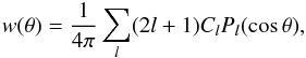$\mathit{w}\mathrm{\left(}\mathit{\theta }\mathrm{\right)}\mathrm{=}\frac{\mathrm{1}}{\mathrm{4}\mathit{\pi }}\sum _{\mathit{l}}\mathrm{(}\mathrm{2}\mathit{l}\mathrm{+}\mathrm{1}\mathrm{)}{\mathit{C}}_{\mathit{l}}{\mathit{P}}_{\mathit{l}}\mathrm{\left(}\cos \mathit{\theta }\mathrm{\right)}\mathit{,}$(8)where P_l(x) are Legendre polynomials. The angular power spectrum C_l of the surface density fluctuation can be calculated from the underlying matter power spectrum, 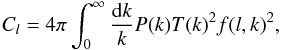${\mathit{C}}_{\mathit{l}}\mathrm{=}\mathrm{4}\mathit{\pi }{\mathrm{\int }}_{\mathrm{0}}^{\mathrm{\infty }}\frac{\mathrm{d}\mathit{k}}{\mathit{k}}\mathit{P}\mathrm{\left(}\mathit{k}\mathrm{\right)}\mathit{T}\mathrm{\left(}\mathit{k}{\mathrm{)}}^{\mathrm{2}}\mathit{f}\mathrm{\right(}\mathit{l,k}{\mathrm{)}}^{\mathrm{2}}\mathit{,}$(9)with P(k) denoting the primordial power spectrum of density fluctuations, T(k) the matter transfer function and $\mathit{f}\mathrm{\left(}\mathit{l,k}\mathrm{\right)}\mathrm{=}\mathrm{\int }\frac{\mathrm{d}\mathit{\sigma ̅}}{\mathrm{d}\mathit{z}}\mathit{b}\mathrm{\left(}\mathit{z}\mathrm{\right)}{\mathit{j}}_{\mathit{l}}\mathrm{\left[}\mathit{ck\eta }\mathrm{\right(}\mathit{z}\mathrm{\left)}\mathrm{\right]}\mathit{D}\mathrm{\left(}\mathit{z}\mathrm{\right)}\mathrm{d}\mathit{z,}$(10)where is the differential number density of sources at flux density above S_t, b(z) denotes the bias, j_ℓ(x) is a spherical Bessel function of first kind, η = η(z) denotes conformal time, and D(z) is the growth factor.

For the galaxy bias, we use the second-order polynomial from the Planck 2015 analysis of the integrated Sachs-Wolfe effect (Planck Collaboration XXI 2016), which is an approximation of the Gaussian bias evolution model of Xia et al. (2010): $\mathit{b}\mathrm{\left(}\mathit{z}\mathrm{\right)}\mathrm{=}\mathrm{0.9}\mathrm{[}\mathrm{1}\mathrm{+}\mathrm{0.54}\mathrm{(}\mathrm{1}\mathrm{+}\mathit{z}{\mathrm{)}}^{\mathrm{2}}\mathrm{]}\mathit{.}$(11)Recently, a detailed analysis of the biasing and evolution of NVSS galaxies was presented by Nusser & Tiwari (2015). Their best-fit bias function is comparable to Eq. (11) up to z ≈ 1.5 and grows slower at larger redshifts. We checked that this difference is insignificant for the purpose of this study. For the additional bias due to non-Gaussianity see Matarrese et al. (2000) and Dalal et al. (2008).

The expected C_l for the NVSS catalogue are obtained using a modified version of the class package (Di Dio et al. 2013). The parameters for the best-fit cosmological model are taken from Planck Collaboration XVI (2014). For the theoretical prediction of the angular two-point correlation we cut the Legendre series at l_max = 900. We convinced ourselves that this cut-off is large enough to ensure numerical convergence of w(θ) at all angular scales considered in this work.

4. Angular two-point correlation of radio galaxies

4.1. Optimal estimation

The angular two-point correlation could be estimated from (Peebles 1980) $\mathrm{1}\mathrm{+}\mathit{w}\mathrm{\left(}\mathit{\theta }\mathrm{\right)}\mathrm{=}\frac{\mathit{DD}}{\mathit{N}\mathrm{(}\mathit{N}\mathrm{+}\mathrm{1}\mathrm{)}\mathit{/}\mathrm{2}}\frac{\mathrm{\Omega }}{\mathrm{⟨}\mathit{\delta }\mathrm{\Omega }\mathrm{⟩}}\mathit{,}$(12)where DD denotes the count of pairs at separation θ and N denotes the total number of objects considered in the analysis. Thus N(N + 1)/2 is the total number of possible pairs, Ω is the solid angle of the survey, and ⟨ δΩ ⟩ is the averaged solid angle of the ring θ to θ + δθ within Ω for a randomly placed ring centre in Ω.

For our analysis we use the optimal estimator found by Landy & Szalay (1993), ${\mathit{w}}_{\mathrm{LS}}\mathrm{\left(}\mathit{\theta }\mathrm{\right)}\mathrm{=}\frac{{\mathit{N}}_{\mathrm{r}}\mathrm{(}{\mathit{N}}_{\mathrm{r}}\mathrm{+}\mathrm{1}\mathrm{)}}{\mathit{N}\mathrm{(}\mathit{N}\mathrm{+}\mathrm{1}\mathrm{)}}\frac{\mathit{DD}}{\overline{\mathit{RR}}}\mathrm{-}\mathit{N}\mathrm{(}{\mathit{N}}_{\mathrm{r}}\mathrm{+}\mathrm{1}\mathrm{)}\frac{\overline{\mathit{DR}}}{\overline{\mathit{RR}}}\mathrm{+}\mathrm{1}\mathit{,}$(13)where $\overline{\mathit{RR}}$ means the averaged pair count over a number of large random simulations, $\overline{\mathit{DR}}$ is the averaged data-random cross pair count for a number of large random simulations, and N_r denotes the number of sources in the random catalogues. It is necessary to clarify that the simulated random sources R have to be identical for $\overline{\mathit{RR}}$ and $\overline{\mathit{DR}}$ to minimize the statistical uncertainty. Under the assumption that higher order correlations among galaxies can be ignored, the Landy-Szalay estimator has a “Poisson error” $\mathit{\delta }{\mathit{w}}_{\mathrm{LS}}\mathrm{\left(}\mathit{\theta }\mathrm{\right)}\mathrm{=}\frac{\mathrm{1}}{\sqrt{\mathit{DD}}}\frac{\mathrm{1}\mathrm{+}{\mathit{w}}_{\mathrm{LS}}\mathrm{\left(}\mathit{\theta }\mathrm{\right)}}{\mathrm{1}\mathrm{+}{\mathit{w}}_{\mathrm{\Omega }}}\mathit{,}$(14)where w_Ω is the mean of the two-point correlation function over the sampling geometry, ${\mathit{w}}_{\mathrm{\Omega }}\mathrm{=}{\mathrm{\int }}_{\mathrm{\Omega }}{\mathit{G}}_{\mathit{p}}\mathrm{\left(}\mathit{\theta }\mathrm{\right)}\mathit{w}\mathrm{\left(}\mathit{\theta }\mathrm{\right)}\mathrm{d\Omega }$(15)where G_p(θ) is a dimensionless geometric form factor which is equal to the fraction of unique cell pairs separated by distance θ ± dθ/ 2 (Landy & Szalay 1993).

In Xia et al. (2010) a pixel based estimator was used (Nside = 64). We compared the Landy-Szalay estimator and the pixel based estimator at Nside = 64 for the same flux threshold and mask. On angular separations above 5 degrees, we found good agreement between both estimators. However, for smaller angular scales it seems that the pixel estimator is redistributing correlation from the smallest scales to intermediate scales. As for Nside = 64 the distance between two neighbor pixel centers is as large as 0.9 deg, it is not surprising that a pixellation error shows up at the few degrees scale.

4.2. Dipole correction

The radio dipole signal is believed to result from our peculiar motion (Ellis & Baldwin 1984) with respect to the cosmic rest frame of radio galaxies, because that the mean redshift of radio galaxies is above one. If this rest frame is the same as the CMB rest frame, then the dipole measured in the radio catalogue should agree with the CMB dipole measured by WMAP and Planck (Jarosik et al. 2011; Planck Collaboration XXVII 2014). Previous studies⁶ (Blake & Wall 2002a; Singal 2011; Gibelyou & Huterer 2012; Rubart & Schwarz 2013; Tiwari et al. 2015; Singal 2014) measured the radio dipole for the NVSS catalogue. It is actually significantly larger than expected, by a factor of two to four depending on the details of the analysis. The origin of this dipole excess is currently unknown. One possibility might be that it is a combination of local large-scale structure (Rubart et al. 2014) and a kinetic component due to Doppler shift and aberration.

A local structure dipole, and the kinetic dipole as well, violate the assumption of statistical isotropy that is implicit in the way we estimate w(θ). We suggest that the dipole signal needs to be taken into account prior to the further correlation or power spectrum analysis. In our analysis the largest contribution to the angular two-point correlation of radio galaxies also comes from the dipole moment of the galaxy distribution, as can be seen in Fig. 8. A significant effect can also be observed for the extracted multipole moments at low l (not shown here).

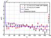Fig. 8 NVSS angular two-point correlations for a 5° galactic latitude mask with and without dipole correction.

Utilizing healpix, we find the radio dipole of the NVSS catalogue after masking with NVSS65 (see Table 2). The estimated dipole at our chosen flux density thresholds and sky coverage agrees with the estimates from the literature (see Rubart 2015 for a recent summary).

The standard dipole subtraction approach for pixelized maps is relatively straightforward. First, we estimate the dipole amplitude and direction through a linear dipole estimator on the pixelized map. Then we subtract the measured dipole contribution at each pixel. However, we do not use the pixel map to measure the correlation function, but rather extract it using the measured positions of all radio sources outside the mask. To achieve this, we have to include the effect of a dipole into the Landy-Szalay estimator.

Thus we simulate random catalogues with the measured dipole, denoted by R_d below, and employ the following estimator, 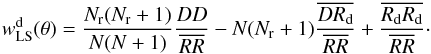${\mathit{w}}_{\mathrm{LS}}^{\mathrm{d}}\mathrm{\left(}\mathit{\theta }\mathrm{\right)}\mathrm{=}\frac{{\mathit{N}}_{\mathrm{r}}\mathrm{(}{\mathit{N}}_{\mathrm{r}}\mathrm{+}\mathrm{1}\mathrm{)}}{\mathit{N}\mathrm{(}\mathit{N}\mathrm{+}\mathrm{1}\mathrm{)}}\frac{\mathit{DD}}{\overline{\mathit{RR}}}\mathrm{-}\mathit{N}\mathrm{(}{\mathit{N}}_{\mathrm{r}}\mathrm{+}\mathrm{1}\mathrm{)}\frac{\overline{\mathit{D}{\mathit{R}}_{\mathrm{d}}}}{\overline{\mathit{RR}}}\mathrm{+}\frac{\overline{{\mathit{R}}_{\mathrm{d}}{\mathit{R}}_{\mathrm{d}}}}{\overline{\mathit{RR}}}\mathrm{·}$(16)The dipole simulations R_d are achieved by the following procedure. First, we assign a uniform random number t to each simulated object and then modify this number based on the angular separation ψ between the object and dipole direction, 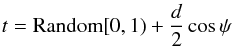$\mathit{t}\mathrm{=}\mathrm{Random}\mathrm{\left[}\mathrm{0}\mathit{,}\mathrm{1}\mathrm{\right)}\mathrm{+}\frac{\mathit{d}}{\mathrm{2}}\cos \mathit{\psi }$(17)Then we add the objects with t ≥ 0.5 to the R_d catalogue and drop the others. Each random catalogue contains N_r = 10⁶ objects and we average over ten such catalogues.

The dipole modified estimator (16) makes use of the full position information of the sources and by simulating several large random catalogues, we minimize the uncertainty in ${\mathit{w}}_{\mathrm{LS}}^{\mathrm{d}}\mathrm{\left(}\mathit{\theta }\mathrm{\right)}$. The computational load is the disadvantage of this procedure.

We can now compare the results with and without dipole subtraction. We either corrected for the measured radio dipole (see Table 2) or for the CMB predicted radio dipole. The dipole contribution in the angular two-point correlation function can be seen from Fig. 8. We find that the dipole has a significant effect and actually dominates the two-point correlation function at large angular scales above ~10°. In the figure we account for the measured dipole. Considering just the CMB predicted dipole reduces the large-angle correlation, but leaves us with a residual dipole that could be due to a local structure and that is hard to predict without a much more detailed study. We therefore decided to correct for the measured NVSS radio dipole and also suppress the structure dipole in the theoretical prediction.

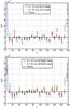Fig. 9 Angular two-point correlation function w(θ) from 5° galactic latitude cut (top panel) and the NVSS65 mask (bottom panel). In both cases we include a dipole correction.

4.3. Results

We adopted the dipole subtracted Landy-Szalay estimator to measure the angular two-point correlations of the NVSS catalogue with thresholds of 15 mJy and 25 mJy for two different masks (NVSS65 and a constant latitude cut of the galactic plane).

The results agree with our expectation. After eliminating the contribution from high rms noise and confusion pixels by means of the NVSS65 mask, the two-point correlation turns out to be less scattered, (see Fig. 9). For the simpler constant latitude cut, the first data point at ~4° is above the plot range of the figure. The NVSS65 mask efficiently reduces the amount of correlation at scales of a few degrees and brings the measurement in agreement with the theoretical expectation of the best-fit cosmological model, and also observe a better agreement of the 15 and 25 mJy thresholded data sets after the NVSS65 mask has been applied. These findings are confirmed by the χ²-values shown in Table 3. We infer that the new NVSS65 mask efficiently pushes the data points towards the theoretical prediction.

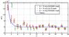Fig. 10 Angular two-point correlation function at 1°<θ< 20° from the NVSS catalogue with dipole correction for two different masks and two different flux thresholds.

Figure 9 also shows that the measurement using the NVSS65 mask agrees with the theoretical prediction until θ ~ 90°. Above that angular scale the data appear to be more noisy. The quite large correlations at the largest angular scales close to 180° are surprising.

For an angular scale between 1° and 20°, the 65% sky coverage guarantees that the w(θ) estimator is averaged over a large number of independent sky patches. Artificial fluctuations caused by the survey or galactic foreground are suppressed in the average, and sidelobes and multicomponent source effects are expected to contaminate smaller angular scales (up to 0.6°). In this range, w(θ) is expected to be consistent with the theoretical prediction.

The result of an analysis at higher angular resolution for θ < 20° is shown in Fig. 10. In order to suppress the shot noise contribution we now focus on the S > 15 mJy data set. We find that the NVSS65 mask improves the agreement with theoretical predictions considerably. At this angular scale, the most important effect of the NVSS65 mask is to remove spurious correlation at θ ≤ 2 deg. We also observed that the NVSS65 mask increases the importance of the dipole subtraction at a separations of a few degrees. As Xia et al. (2010) apply a flux threshold of 10 mJy in their analysis, we also show our corresponding analysis for comparison, however as already discussed above, we think that this flux threshold is not a conservative choice. A discussion of the cosmological consequences is given below.

A complementary analysis to the angular two-point correlation function is to study the angular power spectrum. One way of measuring C_l is to do a Legendre transformation of the angular two-point correlation. The result of that transformation is shown in Fig. 11. Many of the C_l turn out to have negative values, which shows that this measurement is quite noisy. Nevertheless, in the mean the C_l seem to agree well with the theoretical expectations, with exception of a few multipoles with even l, most prominently the l = 10 mode. When restricting the Legendre transformation to the range θ < 100 deg, assuming w(θ) = 0 at θ > 100 deg, we find that the most extreme values, e.g. at ℓ = 10 are suppressed.

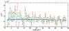Fig. 11 NVSS angular power spectrum Cl for S > 15 mJy, dipole corrected and NVSS65 masked. Cl is evaluated via a Legendre transformation from the angular two-point correlation function (red). The extreme fluctuations are reduced, if the Legendre transformation is limited to θ < 100 deg (green). The solid line and the band around it show the theoretical prediction and its cosmic variance.

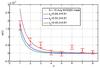Fig. 12 Angular two-point correlation function for different redshift distributions.

5. Discussion

5.1. Cosmological implications

We now turn to the cosmological implications and a discussion of our findings in comparison with previous studies. In the following we focus on the results obtained by means of the NVSS65 mask, including the dipole correction as discussed above and a lower flux threshold of 15 mJy.

A question of interest is the determination of the cosmological parameters of our minimal six-parameter cosmological standard model. For that purpose, the NVSS data alone cannot compete with high fidelity data from the CMB or from optical galaxy redshift surveys. Therefore it is not interesting to determine any of the six cosmological base parameters from a fit to NVSS.

It is important to note that the redshift distribution function also affects the NVSS angular two-point correlation at this angular scale. Figure 12 shows that the parameter z₀ changes its slope and and angular scale. Our angular two-point correlation measurement seems to prefer low z₀ and β, which agrees with the results of Marcos-Caballero et al. (2013).

There is a clear degeneracy between cosmological parameters such as H₀, the redshift distribution parameters (z₀ and β) and the galaxy bias, which limits our ability to use the most recent radio continuum surveys for cosmological parameter estimation. However, it is encouraging that the completely independent measurements of H₀ (Planck), z₀ and β (CENSORS) provide a picture that seems to be consistent with w(θ) from NVSS. In order to extract the full science potential of upcoming radio surveys, a larger sample of redshifts must be measured.

To go beyond the set of the six base parameters, the small angle two-point correlation is also an interesting probe of primordial non-Gaussianity. Previous results (Xia et al. 2010) claimed evidence of a primordial non-Gaussianity at the 3σ level. The angular correlation function is supposed to vanish at around 4° if the fluctuations are Gaussian, but their measurement of w(θ) showed a constant shift from zero at 1°<θ< 10°, which they attributed to the effect of a primordial non-Gaussianity. However, adapting our procedure of masking, dipole correction and optimal estimation of w(θ), we do not see this shift. Our result is consistent with primordial Gaussianity, as is shown in Fig. 10. Turning that into a precise limits on f_nl is beyond the scope of this work.

A primordial non-Gaussianity would also lead to an increase of angular power C_l at low multipoles (Xia et al. 2010; Desjacques & Seljak 2010). The angular power spectrum obtained via a Legendre transformation is shown in Fig. 11. One could be tempted to conclude that we do find an increase of power for low multipoles, similar to Blake et al. (2004) and Marcos-Caballero et al. (2013). However, it should be noted that our method to estimate the angular power spectrum is not optimal and appears to be noisy. On top, most of the excess power is in parity even modes, primordial (local) non-Gaussianity would not care about parity.

We tried to understand what causes for the removal of the apparent non-Gaussianity in the correlation function, but it turns out that it is impossible to attribute it to a single effect. As already discussed in detail above, the essential steps are, using the Landy-Szalay estimator (to avoid pixellation errors), using a larger mask, and removing the dipole contribution.

5.2. Residual systematics

The theoretical prediction based on the ΛCDM model suggested C_l ≈ 5 × 10^-6. Our measurements closely agree with that prediction, with some exceptions. The quadrupole cannot be detected at any significant level and the power at l = 10 is an order of magnitude larger than expected. However, at larger l, up to l ~ 60, the C_l are consistent with the theoretical prediction, which is in agreement with previous analyses of the ISW effect Hernández-Monteagudo (2010). Higher multipole moments are noisy and statistically consistent with zero.

We finally discuss the angular scales at θ > 20° and look in more detail at the corresponding multipole moments up to l = 10. For a simple galactic isolatitude cut, we find significantly more power at low multipole moments, with l = 4 being the dominant mode (not discussed here). The essential way to get rid of this extra power is to take direction dependent systematic effects into account in the NVSS catalogue. Our NVSS65 mask allows us to reduce the l = 4 mode and to recover an overall flat angular power spectrum. However, even with the NVSS65 mask, some of the C_ls are one order of magnitude larger than the prediction at l < 10. Perhaps because of remaining surface density fluctuations at different declinations.

We find a clear anti-correlation between the surface density and the theoretical rms noise of the NVSS catalogue, Fig. 13. The declination dependence of the theoretical rms noise fluctuations at −40° <δ < −10° is due to changes in the snapshot integration time. When the VLA points to the horizon, the effect of the projection of the uv plane combined with ground and ionospheric noise decreases the effective signal-to-noise ratio of the survey. As can be seen in Fig. 13 this effect is not limited to the faintest sources, but is also there for brighter sources at S > 60 mJy. Thus, only the most extreme influence of the direction dependent systematics can be cured by means of a lower flux threshold.

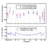Fig. 13 Top panel: surface density fluctuation ($\mathrm{\Delta }\mathit{\sigma }\mathit{/}\overline{\mathit{\sigma }}$) of NVSS sources at S > 60 mJy and S > 15 mJy after applying the NVSS65 mask. Bottom panel: the theoretical rms noise level of the NVSS catalogue from Condon et al. (1998). The VLA geodetic latitude is 34°04′44′′.

To further probe whether these direction dependent effects affect the low-l multipoles, we investigated the angular pseudo-power spectra, which are obtained through a decomposition into spherical harmonics on the pixelized galaxy number count. For this we used healpix. In Fig. 14 we show estimates of the pseudo-C_l for two different normalizations. In the first case, we normalize the pixel count with the mean pixel count of the full survey , i.e. ${\mathit{x}}_{\mathit{i}}\mathrm{=}\frac{{\mathit{n}}_{\mathit{i}}\mathrm{-}\mathit{n̅}}{\mathit{n̅}}\mathrm{·}$(18)The second case is motivated by Vielva et al. (2006). We divide the map along the declination, based on durations of the snapshots, and subtract the mean pixel count at declination δ_i, ${\mathit{x}}_{\mathit{i}}\mathrm{=}\frac{{\mathit{n}}_{\mathit{i}}\mathrm{-}\mathit{n̅}{\mathit{\delta }}_{\mathit{i}}}{\mathit{n̅}}\mathrm{·}$(19)This procedure was also used in the Planck analysis of the ISW effect (Planck Collaboration XIX 2014; Planck Collaboration XXI 2016).

This second procedure, erases the source density fluctuations along the declination direction. As can be seen in Fig. 14, the l = 3,4,5 multipoles are significantly reduced by the declination mean subtraction, which strongly implies that the l = 4 mode fluctuations are caused by the direction dependent noise of the NVSS catalogue. On the other hand, the large l = 10 mode is not affected by that normalization at all and it is not clear why it exceeds the expectation by an order of magnitude. Using this declination normalization for a cosmological analysis, such as Vielva et al. (2006), Fernández-Cobos et al. (2014) or Planck Collaboration XIX (2014), certainly suppresses fluctuations on large scales, but the procedure cannot distinguish direction dependent effects from real fluctuations and it is very hard to assign an error estimate to it.

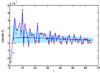Fig. 14 The healpix pseudo-Cl of the NVSS catalogue with NVSS65 mask for S > 15 mJy and radio dipole subtracted. The zig-zag line shows the standard normalization. The crosses show the declination normalization result. The smooth solid line shows the theoretical prediction and the band around it includes shot noise and cosmic variance.

To analyse this effect in more detail, we took the S > 10 mJy, |b| < 5 degree map before dipole subtraction and used the same pixel estimator as in Xia et al. (2010; including only full pixels) as a baseline in Fig. 15. This baseline seems to have some excess power. We found that both the strip normalization and the dipole subtraction give a substantial reduction and almost identical results. We thus think that it would be better to just subtract the dipole and to use a more conservative mask or carefully modeling this systematic effect, instead of setting all fluctuations between declination strips to zero.

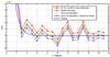Fig. 15 Pixel based estimate of the angular correlation function of the NVSS catalogue for S > 10 mJy with |b| < 5 mask (red line). The effects of dipole removal (green) and declination normalisation (brown) are shown for comparison. The purple line shows the result using a declination normalization and subsequent dipole subtraction.

In addition, we note a curious observation. Looking carefully at Fig. 11, we observe a parity asymmetry in the C_l: the power of even multipoles l = 4,8,10,12,16,22,24,32... is higher than that of their odd neighbours. This even parity preference can also be seen because w(180°) > 0. A similar effect was observed in the CMB angular power spectrum, where the parity asymmetry is the opposite Kim & Naselsky (2010). There the odd l(l + 1)C_l/ 2πs are larger than the even ones.

Our results further suggest that w(θ) from full-sky radio continuum surveys can be used to constrain cosmological parameters at an epoch that is barely accessible to other probes. Planned and upcoming surveys with instruments like LOFAR, ASKAP, MeerKAT and finally SKA will allow us to reduce the shot noise and to increase angular resolution and sensitivity, while covering all sky, extending the studies to several frequency bands (our discussion here is limited to 1.4 GHz), and improving the control of systematic effects. For more details see Raccanelli et al. (2012) and Jarvis et al. (2015) and references therein.

6. Conclusion

In this paper we revisited the angular two-point correlation function w(θ) and angular power spectrum C_l from the NVSS catalogue of radio galaxies. The focus of our work was to investigate systematic effects in the NVSS catalogue. In order to minimize the contribution of these effects in the cosmological analysis, we provide a new NVSS mask with 64.7% percent of sky, called NVSS65. We also find that it is essential to account for the radio dipole and to use an optimal estimator. We found that our mask significantly improves the χ² value of the angular two-point correlation function on all angular scales. For angular scales between 1 and 20 deg, w(θ) agrees with the flat ΛCDM model without introducing primordial non-Gaussianity.

Thus we have shown that to fully explore the cosmological potential of continuum radio surveys, one has to understand and investigate the systematic effects related to flux calibration, especially direction dependent effects of the calibration. In addition, the effect of the cosmic radio dipole affects the reconstruction of higher multipole moments and the attempts to measure or constrain primordial non-Gaussianity.

To obtain an improved upper limit on f_nl or to constrain other cosmological parameters at a redshift of about unity is beyond the scope of this work, as it would need an extensive study of the uncertainties coming from our understanding of the density, luminosity and bias evolution of radio galaxies. However, our analysis shows that the radio sky is in remarkably good agreement with the standard model of cosmology according to Planck. It will also be interesting to improve the ISW analysis of the Planck-NVSS cross-correlation by means of the new NVSS65 mask, and to include a radio dipole correction, as well as a higher flux threshold.

Acknowledgments

We thank Anne-Sophie Balleier, Daniel Boriero, Bin Hu, Dragan Huterer, Hans-Rainer Klöckner, Alvise Raccanelli, and Matthias Rubart for valuable comments and discussions. We acknowledge financial support from Deutsche Forschungsgemeinschaft (DFG) via the Research Training Group “Models of Gravity” (RTG 1620). We are grateful for the possibility of performing the numerical computations on the Nordrhein-Westfalen state computing cluster at RWTH Aachen. We acknowledge the use of the NVSS catalogue Condon et al. (1998), provided by the NRAO. This work made extensive use of the healpixGorski et al. (2005) and the classLesgourgues & Tram (2011), Di Dio et al. (2013) packages.

References

All Tables

All Figures

	Fig. 1 Surface density of the NVSS source catalogue in galactic coordinates in Mollweide projection, shown at healpix resolution Nside = 32. The colour bar shows the surface density in units of number of objects per square degree. Here we include all objects contained in the catalogue. The white dots indicate the the positions of the celestial poles.
In the text

	Fig. 2 Surface density fluctuation, $\mathrm{\Delta }\mathit{\sigma }\mathit{/}\overline{\mathit{\sigma }}$, of the NVSS catalogue as a function of declination for several flux density thresholds. The error bars assume Poisson distributed source counts and we mask the region | b | ≤ 5°. For clarity, the horizontal positions of the S> 5 mJy and S> 15 mJy data points are slightly offset.
In the text

	Fig. 3 Cumulative distribution of nearby source counts (disks with radius 0.6°). The red line corresponds to nearby source counts around bright radio galaxies with S> 2.5 Jy. The blue line corresponds to 1000 randomly picked positions outside the galactic plane (| b | > 5°). The maximum of randomly picked counts results in 49 nearby sources.
In the text

	Fig. 4 Poissonness plot of the nearby source counts. λo is the mean nearby count over the survey area. N is the total number of sources with S> 2.5 Jy. The solid horizontal line corresponds to a perfectly Possion distributed nearby source count. The error bars denote the 99% confidence levels.
In the text

	Fig. 5 NVSS position uncertainty map, relative to the mean beam width θFWHM = 45′′.
In the text

	Fig. 6 NVSS65 mask. The orange region makes up 64.7% of the sky. Yellow pixels are close to the galactic plane | b | ≤ 5° and are excluded to suppress galactic point sources and foregrounds. Blue pixels are excluded owing to large position errors. Red and black pixels contain bright sources with significant sidelobe effects; black pixels also overlap with pixels with high position error.
In the text

	Fig. 7 Surface density of the NVSS source catalogue for a flux density threshold of S> 15 mJy and applying the NVSS65 mask, shown in galactic coordinates at pixel size Nside=32. The colour bar shows the surface density σ in units of number of objects per square degree.
In the text

	Fig. 8 NVSS angular two-point correlations for a 5° galactic latitude mask with and without dipole correction.
In the text

	Fig. 9 Angular two-point correlation function w(θ) from 5° galactic latitude cut (top panel) and the NVSS65 mask (bottom panel). In both cases we include a dipole correction.
In the text

	Fig. 10 Angular two-point correlation function at 1°<θ< 20° from the NVSS catalogue with dipole correction for two different masks and two different flux thresholds.
In the text

	Fig. 11 NVSS angular power spectrum Cl for S > 15 mJy, dipole corrected and NVSS65 masked. Cl is evaluated via a Legendre transformation from the angular two-point correlation function (red). The extreme fluctuations are reduced, if the Legendre transformation is limited to θ < 100 deg (green). The solid line and the band around it show the theoretical prediction and its cosmic variance.
In the text

	Fig. 12 Angular two-point correlation function for different redshift distributions.
In the text

	Fig. 13 Top panel: surface density fluctuation ($\mathrm{\Delta }\mathit{\sigma }\mathit{/}\overline{\mathit{\sigma }}$) of NVSS sources at S > 60 mJy and S > 15 mJy after applying the NVSS65 mask. Bottom panel: the theoretical rms noise level of the NVSS catalogue from Condon et al. (1998). The VLA geodetic latitude is 34°04′44′′.
In the text

	Fig. 14 The healpix pseudo-Cl of the NVSS catalogue with NVSS65 mask for S > 15 mJy and radio dipole subtracted. The zig-zag line shows the standard normalization. The crosses show the declination normalization result. The smooth solid line shows the theoretical prediction and the band around it includes shot noise and cosmic variance.
In the text

	Fig. 15 Pixel based estimate of the angular correlation function of the NVSS catalogue for S > 10 mJy with |b| < 5 mask (red line). The effects of dipole removal (green) and declination normalisation (brown) are shown for comparison. The purple line shows the result using a declination normalization and subsequent dipole subtraction.
In the text

References

- Bennett, C. L., Hill, R. S., Hinshaw, G., et al. 2011, ApJS, 192, 17 [NASA ADS] [CrossRef] [Google Scholar]
- Blake, C., & Wall, J. 2002a, Nature, 416, 150 [NASA ADS] [CrossRef] [Google Scholar]
- Blake, C., & Wall, J. 2002b, MNRAS, 329, L37 [NASA ADS] [CrossRef] [Google Scholar]
- Blake, C., Ferreira, P. G., & Borrill, J. 2004, MNRAS, 351, 923 [NASA ADS] [CrossRef] [Google Scholar]
- Brookes, M., Best, P., Peacock, J., Rottgering, H., & Dunlop, J. 2008, MNRAS, 385, 1297 [NASA ADS] [CrossRef] [Google Scholar]
- Chen, S., & Schwarz, D. J. 2015, ArXiv e-prints [arXiv:1507.02160] [Google Scholar]
- Condon, J. J., Cotton, W. D., Greisen, E. W., et al. 1998, ApJ, 115, 1693 [Google Scholar]
- Copi, C. J., Huterer, D., Schwarz, D. J., & Starkman, G. D. 2010, Adv. Astron., 2010, 78 [NASA ADS] [CrossRef] [Google Scholar]
- Copi, C. J., Huterer, D., Schwarz, D. J., & Starkman, G. D. 2015a, MNRAS, 449, 3458 [NASA ADS] [CrossRef] [Google Scholar]
- Copi, C. J., Huterer, D., Schwarz, D. J., & Starkman, G. D. 2015b, MNRAS, 451, 2978 [NASA ADS] [CrossRef] [Google Scholar]
- Dalal, N., Doré, O., Huterer, D., & Shirokov, A. 2008, Phys. Rev. D, 77, 123514 [NASA ADS] [CrossRef] [Google Scholar]
- de Zotti, G., Massardi, M., Negrello, M., & Wall, J. 2010, A&ARv, 18, 1 [NASA ADS] [CrossRef] [Google Scholar]
- Desjacques, V., & Seljak, U. 2010, Class. Quant. Grav., 27, 124011 [NASA ADS] [CrossRef] [Google Scholar]
- Di Dio, E., Montanari, F., Lesgourgues, J., & Durrer, R. 2013, J. Cosmol. Astropart. Phys., 1311, 044 [CrossRef] [Google Scholar]
- Ellis, G. F. R., & Baldwin, J. E. 1984, MNRAS, 206, 377 [NASA ADS] [CrossRef] [Google Scholar]
- Fernández-Cobos, R., Vielva, P., Pietrobon, D., et al. 2014, MNRAS, 441, 2392 [NASA ADS] [CrossRef] [Google Scholar]
- Gibelyou, C., & Huterer, D. 2012, MNRAS, 427, 1994 [NASA ADS] [CrossRef] [Google Scholar]
- Gorski, K., Hivon, E., Banday, A., et al. 2005, ApJ, 622, 759 [NASA ADS] [CrossRef] [Google Scholar]
- Hernández-Monteagudo, C. 2010, A&A, 520, A101 [NASA ADS] [CrossRef] [EDP Sciences] [Google Scholar]
- Ho, S., Hirata, C., Padmanabhan, N., Seljak, U., & Bahcall, N. 2008, Phys. Rev. D, 78, 043519 [NASA ADS] [CrossRef] [Google Scholar]
- Hoaglin, D. C., & Tukey, J. W. 2006, Exploring Data Tables, Trends, and Shapes (John Wiley & Sons, Inc) [Google Scholar]
- Jarosik, N., Bennett, C., Dunkley, J., et al. 2011, ApJS, 192, 14 [NASA ADS] [CrossRef] [Google Scholar]
- Jarvis, M., Bacon, D., Blake, C., et al. 2015, PoS, AASKA14, 018 [Google Scholar]
- Kim, J., & Naselsky, P. 2010, ApJ, 714, L265 [NASA ADS] [CrossRef] [Google Scholar]
- Landy, S. D., & Szalay, A. S. 1993, ApJ, 412, 64 [NASA ADS] [CrossRef] [Google Scholar]
- Lesgourgues, J., & Tram, T. 2011, J. Cosmol. Astropart. Phys., 1109, 032 [Google Scholar]
- Maartens, R., Zhao, G.-B., Bacon, D., Koyama, K., & Raccanelli, A. 2013, J. Cosmol. Astropart. Phys., 1302, 044 [NASA ADS] [CrossRef] [Google Scholar]
- Marcos-Caballero, A., Vielva, P., Martinez-Gonzalez, E., et al. 2013, ArXiv e-prints [arXiv:1312.0530] [Google Scholar]
- Matarrese, S., Verde, L., & Jimenez, R. 2000, ApJ, 541, 10 [NASA ADS] [CrossRef] [Google Scholar]
- Naselsky, P., Zhao, W., Kim, J., & Chen, S. 2012, ApJ, 749, 31 [NASA ADS] [CrossRef] [Google Scholar]
- Nusser, A., & Tiwari, P. 2015, ApJ, 812, 85 [NASA ADS] [CrossRef] [Google Scholar]
- Peebles, P. 1980, The Large-Scale Structure of the Universe (Princeton Univ. Press) [Google Scholar]
- Planck Collaboration XIX. 2014, A&A, 571, A19 [NASA ADS] [CrossRef] [EDP Sciences] [Google Scholar]
- Planck Collaboration XVI. 2014, A&A, 571, A16 [NASA ADS] [CrossRef] [EDP Sciences] [Google Scholar]
- Planck Collaboration XXIII. 2014, A&A, 571, A23 [NASA ADS] [CrossRef] [EDP Sciences] [MathSciNet] [PubMed] [Google Scholar]
- Planck Collaboration XXVII. 2014, A&A, 571, A27 [NASA ADS] [CrossRef] [EDP Sciences] [Google Scholar]
- Planck Collaboration XVI. 2016, A&A, in press, DOI: 10.1051/0004-6361/201526681 [Google Scholar]
- Planck Collaboration XXI. 2016, A&A, in press, DOI: 10.1051/0004-6361/201525831 [Google Scholar]
- Raccanelli, A., Zhao, G.-B., Bacon, D. J., et al. 2012, MNRAS, 424, 801 [NASA ADS] [CrossRef] [Google Scholar]
- Rubart, M. 2015, Ph.D. Thesis, University Bielefeld [Google Scholar]
- Rubart, M., & Schwarz, D. J. 2013, A&A, 555, A117 [NASA ADS] [CrossRef] [EDP Sciences] [Google Scholar]
- Rubart, M., Bacon, D., & Schwarz, D. J. 2014, A&A, 565, A111 [NASA ADS] [CrossRef] [EDP Sciences] [Google Scholar]
- Singal, A. K. 2011, ApJ, 742, L23 [NASA ADS] [CrossRef] [Google Scholar]
- Singal, A. K. 2014, A&A, 568, A63 [NASA ADS] [CrossRef] [EDP Sciences] [Google Scholar]
- Tiwari, P., Kothari, R., Naskar, A., Nadkarni-Ghosh, S., & Jain, P. 2015, Astropart. Phys., 61, 1 [NASA ADS] [CrossRef] [Google Scholar]
- Vielva, P., Martínez-González, E., & Tucci, M. 2006, MNRAS, 365, 891 [NASA ADS] [CrossRef] [Google Scholar]
- Xia, J.-Q., Viel, M., Baccigalupi, C., et al. 2010, ApJ, 717, L17 [NASA ADS] [CrossRef] [Google Scholar]
All Tables
χ2-values testing for the isotropy in declination of the NVSS surface density after masking the region | b | ≤ 5° and for 13 degrees of freedom.
NVSS dipole for various flux density thresholds, measured by means of healpix at resolution Nside = 32 after applying the NVSS65 mask.