| Issue |
A&A
Volume 591, July 2016
|
|
|---|---|---|
| Article Number | A57 | |
| Number of page(s) | 15 | |
| Section | Stellar structure and evolution | |
| DOI | https://doi.org/10.1051/0004-6361/201526726 | |
| Published online | 13 June 2016 | |
The different origins of magnetic fields and activity in the Hertzsprung gap stars, OU Andromedae and 31 Comae⋆
1 Institute of Astronomy, Bulgarian Academy of Sciences, 71 Tsarigradsko Shosse blvd, 1784 Sofia, Bulgaria
e-mail: This email address is being protected from spambots. You need JavaScript enabled to view it.
2 Université de Toulouse, UPS-OMP, Institut de Recherche en Astrophysique et Planétologie, 31400 Toulouse, France
3 CNRS, UMR 5277, Institut de Recherche en Astrophysique et Planétologie, 14 Av. Édouard Belin, 31400 Toulouse, France
4 Department of Astronomy, University of Geneva, Chemin des Maillettes 51, 1290 Versoix, Switzerland
5 Saint Petersburg State University, Saint Petersburg, Universitetski pr. 28, 198504 Saint Petersburg, Russia
6 Observatório Nacional/MCTI, Rua General José Cristino 77, 20921-400 Rio de Janeiro, Brazil
Received: 12 June 2015
Accepted: 20 March 2016
Abstract
Context. When crossing the Hertzsprung gap, intermediate-mass stars develop a convective envelope. Fast rotators on the main sequence, or Ap star descendants, are expected to become magnetic active subgiants during this evolutionary phase.
Aims. We compare the surface magnetic fields and activity indicators of two active, fast rotating red giants with similar masses and spectral class but different rotation rates – OU And (Prot = 24.2 d) and 31 Com (Prot = 6.8 d) – to address the question of the origin of their magnetism and high activity.
Methods. Observations were carried out with the Narval spectropolarimeter in 2008 and 2013. We used the least-squares deconvolution (LSD) technique to extract Stokes V and I profiles with high signal-to-noise ratio to detect Zeeman signatures of the magnetic field of the stars. We then provide Zeeman-Doppler imaging (ZDI), activity indicators monitoring, and a precise estimation of stellar parameters. We use state-of-the-art stellar evolutionary models, including rotation, to infer the evolutionary status of our giants, as well as their initial rotation velocity on the main sequence, and we interpret our observational results in the light of the theoretical Rossby numbers.
Results. The detected magnetic field of OU Andromedae (OU And) is a strong one. Its longitudinal component Bl reaches 40 G and presents an about sinusoidal variation with reversal of the polarity. The magnetic topology of OU And is dominated by large-scale elements and is mainly poloidal with an important dipole component, as well as a significant toroidal component. The detected magnetic field of 31 Comae (31 Com) is weaker, with a magnetic map showing a more complex field geometry, and poloidal and toroidal components of equal contributions. The evolutionary models show that the progenitors of OU And and 31 Com must have been rotating at velocities that correspond to 30 and 53%, respectively, of their critical rotation velocity on the zero age main sequence. Both OU And and 31 Com have very similar masses (2.7 and 2.85 M⊙, respectively), and they both lie in the Hertzsprung gap.
Conclusions. OU And appears to be the probable descendant of a magnetic Ap star, and 31 Com the descendant of a relatively fast rotator on the main sequence. Because of the relatively fast rotation in the Hertzsprung gap and the onset of the development of a convective envelope, OU And also has a dynamo in operation.
Key words: stars: individual: OU Andromedae / stars: individual: 31 Comae / stars: late-type / stars: magnetic field
Based on observations obtained at the telescope Bernard Lyot (TBL) at Observatoire du Pic du Midi, CNRS/INSU and Université de Toulouse, France.
© ESO, 2016
1. Introduction
Recent studies report the detection of magnetic fields with strengths that range from a few tenths to a hundred gauss at the surface of single red giants of intermediate mass (Konstantinova-Antova et al. 2014; Aurière et al. 2015). This raises the question of the origin and evolution of magnetic fields during the stellar evolution. An interesting evolutionary stage is the subgiant phase. When intermediate mass stars leave the main sequence and cross the Hertzsprung gap, they develop a convective envelope, and their surface rotation rate decreases as a consequence of the increase of their radius. In ordinary giant stars, α−ω dynamo is then favored during the so-called first dredge-up at the base of the red giant branch, owing to structural changes of the convective envelope that imply an increase of the convective turnover timescale and a temporary decrease of the Rossby number (so-called magnetic strip, see Charbonnel et al. 2016; Aurière et al. 2015); in parallel at that phase, the large-scale fossil magnetic field of Ap star descendants has not yet been strongly diluted. A number of Hertzsprung gap-crossers are detected in X-rays as active stars (Gondoin 1999, 2005a; Ayres et al. 1998, 2007). For these stars, magnetic activity is a result of a remnant of relatively fast rotation, because the convective envelope is not yet well developed.
Fundamental parameters for OU And and 31 Com.
An essential point is to distinguish between descendants of stars hosting strong fossil magnetic fields on the surface of the main sequence (magnetic Ap stars) and the ones generating their magnetic field as a result of their evolution during the Hertzsprung gap. In this paper we present a study of the magnetism and activity of two subgiant stars, OU And and 31 Com, that are very similar in terms of mass, spectral type, activity properties, evolutionary stage (i.e., they both lie in the Hertzsprung gap stepping up to the edge of the so-called magnetic strip), and strong X-ray activity, but which have significantly different rotational rates.
OU And (HD 223460, HR 9024) is a single, G1 III giant (Gray et al. 2001) with moderate emission in Ca ii H&K line (Cowley & Bidelman 1979). It is a moderate rotator with vsini ~ 21 km s-1 for its position in the Herzsprung gap with Teff ~ 5360 K and M = 2.85 M⊙ (see Table 1 and Sect. 5.1). The photometric variability of the star was discovered by Hopkins et al. (1985) who determined a photometric period 23.25 ± 0.09 d. Strassmeier & Hall (1988) provided a long-term monitoring of the brightness of the star and confirmed that the photometric period and light curve amplitude undergoes smooth changes. They estimated a photometric period of 22.6 ± 0.09 d. The latest photomeric data of the star are presented by Strassmeier et al. (1999) and reveal an uncertain period of 24.2 days and V amplitude of about 0.01 mag. Amplitude and period changes, as in OU And, are also observed in other chromospherically active giants and may indicate cyclic activity like in the Sun. OU And is chromospherically active with X-ray luminosity variations. Series of highly ionised iron lines, several Lyman lines of hydrogen-like ions and triplet lines of Helium-like ions in the X-ray region (Gondoin 2003; Ayres et al. 2007) are observed in its spectra.
31 Com (HD 111812) is a single G0 III, (Gray et al. 2001), rapidly rotating giant with vsini ~ 67 km s-1, Teff ~ 5660 K and M = 2.75 M⊙ (Strassmeier et al. 2010, see Table 1 and Sect. 5.1). The star is a variable with a very low light curve amplitude and rotational modulation with a period of ~ 6.8 d. Its light curve appears to be complex, with period and shape changes and multiple peaks in the periodogram (Strassmeier et al. 2010). The star shows chromospheric and coronal activity with Ca ii H&K line emission, super-rotationally broadened coronal and transition-region lines, and strong X-ray activity (Gondoin 2005a).
Table 1 summarizes the fundamental parameters for OU And and 31 Com which we have used in this paper, with their relevant references. The stellar radius is obtained from the Stefan-Boltzmann law using the adopted values for the stellar effective temperature and luminosity.
Spectropolarimetric observations, activity indicators and Bl measurements for 31 Com in 2013.
2. Observations and data processing
Observations were carried out with the Narval spectropolarimeter of the 2 m telescope Bernard Lyot at Pic du Midi Observatory, France, during two consecutive semesters of 2013. 31 Com was observed in the first semester of 2013 during 10 nights of April and May, while OU And was observed in the second semester of 2013, during 13 nights in September and October. Additionally, we used six OU And observations obtained with the same instrumental configuration in September 2008. The total exposure time for each observation of OU And was 40 min with the exception of the first two observations : on 14 September 2008 it was 4 min and on 16 September 2008 it was 16 min.The total exposure time for each observation of 31 Com was ~ 33.3 min. Detailed information for these observations is presented in Tables 2 and 3 for OU And and 31 Com, respectively. Observational data obtained in 2013 for OU And were collected during three rotations of the star, while for 31 Com they were collected in four stellar rotations. In 2013, we obtained relatively good phase coverage for OU And, with some small phase gaps near phases 0.6 and 0.9. The observational data set for 31 Com suffers from one large data -gap, of about 40% of the rotational cycle.
Narval is a twin of ESPaDOnS spectropolarimeter (Donati et al. 2006a). This consists of a polarimetric unit connected by optical fibers to a cross–dispersed échelle spectrometer. The instrument has high-resolution (R = λ∕Δλ ≃ 65 000) and wavelength coverage from about 369 to 1048 nm. In the spectropolarimetric mode two orthogonally polarized spectra are recorded in a single exposure over the whole spectral band. We obtained standard circular-polarization observations that consist of a series of four sub-exposures, between which the half-wave retarders (Fresnel rhombs) are rotated to change paths (and the spectra positions on the CCD) of the two orthogonally polarized light beams. This way the spurious polarization signatures are reduced. Typically diagnostic null spectra N are also included in the observational data. In principle, these spectra should not contain polarization signatures and serve to ensure the absence of any spurious signal in the Stokes V spectra.
The data were reduced using the Libre ESpRIT (Donati et al. 1997) software for automatic spectra extraction. The software includes wavelength calibration, heliocentric frame correction, and continuum normalization. Afterwards, a data reduction extracted spectra are recorded in an ASCII file and they consist of the normalized Stokes I (I/Ic) and Stokes V (V/Ic) intensities and the Stokes V uncertainty, σv as a function of wavelength, (where Ic represents the continuum level).
The least-squares deconvolution method, (here and after – LSD, Donati et al. 1997) was applied to all of the observations to perform extraction of the mean Stokes V and Stokes I photospheric profiles. This is a multi-line analysis method and assumes that all the spectral lines have the same profile, scaled by a certain factor and that the observed spectrum can be represented as a convolution of single mean line profile with the so-called line mask. In the case of cool stars, this technique usually averages several thousand spectral lines and thus significantly increases the signal-to-noise ratio (S/N) in the mean line profile. The line mask was computed by the use of spectral synthesis based on the Kurucz (1993) models, and represented theoretical spectrum of unbroadened spectral lines with appropriate wavelength, depth, and Lande factor, Donati et al. (1997). For the present observations, we used a digital mask calculated for an effective temperature of 5750 K and log g = 3.5 and with about 8900 spectral lines for both stars. We used the atomic transition data provided by the VALD database, Kupka et al. (2000). Owing to the LSD technique the S/N in the Stokes V profiles for both stars was increased by about 40 times. This is presented in the last column of Tables 2 and 3.
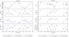 |
Fig. 1 Bl, S-index, Hα, and Ca ii IR triplet indexes behavior for OU And (left) and 31 Com (right). For both stars, phases are computed for ephemeris HJD0 = 2 454 101.5 and the rotational period of 24.2 d for OU And and 6.8 d for 31 Com. |
3. Magnetic field detection and strength. Activity indicators behavior
The output of the LSD procedure contains the mean Stokes V and I, the diagnostic null (N) profile, as well as a statistical test for the detection of Zeeman signatures in Stokes V profiles. The test is performed inside and outside spectral lines and estimates the magnetic field detection probabilities, as described by Donati et al. (1992, 1997). The “definite detection” is assumed if the probability for signal detection in the spectral line is greater than 99.999%, “marginal detection” – if it falls in the range 99.9% and 99.999%, and no detection otherwise. We examine the signal in the N profile and also outside the spectral line and for a reliable detection the one without a signal in the latter two is accepted. Mean surface-averaged longitudinal magnetic field (Bl, G) was computed by the use of the first order moment method (Rees & Semel 1979), adapted to LSD profiles (Donati et al. 1997; Wade et al. 2000).
The activity of the stars were also examined using traditional spectral activity indicators, Ca ii H&K, S-index, Hα, and Ca IR triplet indexes, Marsden et al. (2014). We calculated the S-index as it is defined for the Mount Wilson survey (Duncan et al. 1991) and our computational procedure was calibrated for Narval spectra, see Aurière et al. (2015). The Hα and Ca ii IR triplet indexes are introduced by Gizis et al. (2002) for the Palomar Nearby Spectroscopic Survey and by Petit et al. (2013) for the Betelgeuse cool supergiant, respectively. In this study, we used a slightly modified Hα index with the continuum taken slightly farther from the line center to avoid the influence of broadening that is due to the active chromosphere and fast rotation.
Observational results for detected magnetic field and for the activity indicators are presented in Tables 2 and 3, as well as in Fig. 1. The tables columns are: Date of observation, HJD, rotational phases, S/N in LSD Stokes V profile, S-index, Hα index, Ca ii IR index, Bl, and the corresponding accuracy in G. Rotational phases are computed for ephemeris HJD0 = 2 454 101.5 and rotational period of 24.2 d for OU And and 6.8 d for 31 Com. Preferred choice for the rotational period of OU And is discussed in Sect. 4.2.
Figure 1 represents Bl, S-index, Hα, and Ca ii IR triplet indexes for OU And (in 2013) on the left panel and for 31 Com on the right panel. Activity indicators and Bl plots for OU And in 2008 are presented in Fig. 6. Rotational phases are computed the same way as for Fig. 1. For OU And, the error bars on the plots are of about the same size as the plot symbol and they are not visible. We have definite magnetic field detection for all the spectra, except for one of 31 Com, which was obtained on the 20 April 2013 with a marginal detection. OU And data reveal a strong Zeeman signature in the Stokes V profile with a structure that has several peaks, while for 31 Com we have got relatively weaker signatures, with strong noise contribution and a much more complex structure.
For OU And, the longitudinal magnetic field, Bl, shows a very good rotational modulation and we have well-sampled data at the minimum Bl. The maximal values of Bl are not well covered with data. We observe anticorrelation between the Bl and Hα index. There is also a good correlation between the two Calcium indexes, which indicates that the measurements really concern the Ca ii contribution. There is some scatter between the different rotations for the activity indicators, although not for the magnetic field. For most activity proxies, some scatter is observed between successive rotation cycles. The measurements obtained at different stellar rotations agree much better for the longitudinal magnetic field.
For 31 Com we see clear Bl minimum and a smooth variation with rotation. However, because the longitudinal field estimates result from an integration over the full width of the line profile, they do not therefore capture the full complexity of the Stokes V profile, and hence the magnetic structure. The indexes show a good correlation, but we have a large data gap between phases 0.2 and 0.5. The S-index and Ca ii IR triplet index show a decrease in the third rotation. The Bl measurement on 20 April 2013 is excluded because of the marginal magnetic field detection.
4. Magnetic mapping
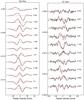 |
Fig. 2 Observed Stokes V LSD profiles (black line) and profiles produced by our best ZDI model (red lines) for OU And (left) and 31 Comae (right). Successive profiles are vertically shifted (from top to bottom) for display clarity. The rotational phase of each observation (computed from the ephemeris given in the text) is listed to the right, with the integer part denoting the rotational cycle since the start of the observing run. Error bars are illustrated on the left of every profile and dashed lines illustrate the zero level. |
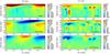 |
Fig. 3 Photospheric magnetic maps of OU And (left) and 31 Com (right) in 2013. For each star, the vectorial magnetic field is split in its three components in spherical projection and ℓmax = 20. The color scale illustrates the field strength in Gauss, and the rotational phases of our data sets show up as vertical ticks on top of each map. |
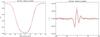 |
Fig. 4 Evolution of Stokes I and Stokes V (left and right, respectively) LSD profiles of OU And observed close to phase 0.4. We represent in black the observation of 2013 Sept. 19 (phase 0.41) and in red the observation of 2013 Oct. 13 (phase 0.40). |
The temporal series of observations gathered for both stars offer the opportunity to obtain polarized measurements at various rotational phases. Using this multi-angle view of the stellar photosphere, tomographic methods can be used to model the surface magnetic geometry of the targets.
4.1. Zeeman-Doppler imaging
The tomographic algorithm employed here is based on the Zeeman-Doppler imaging (ZDI) method proposed by Semel (1989). More specifically, we use the maximum-entropy ZDI code described by Donati et al. (2006b). The ZDI principle makes use of the fact that the Doppler broadening of the polarized profiles results in a 1D resolution of the stellar surface (orthogonally to the rotation axis), as magnetic spots located at different places on the visible stellar hemisphere possess different radial velocities and, therefore, produce polarized spectral signatures showing up with a different wavelength shift with respect to the line center. The succession of observations gathered at different rotational phases is then used to recover the full surface distribution of the local magnetic vector, by iterative adjustment of the time-series of LSD profiles.
The synthetic LSD profiles produced by ZDI rely on a simplified atmospheric model, based on a spherical artificial star split into a grid of pixels of roughly identical areas. Each pixel is attributed a brightness that we assume to be constant over stellar surface (but affected by limb darkening), and the elemental areas host a magnetic field with a given strength and orientation. Each pixel produces Stokes I and V spectral lines, computed under the weak-field approximation (which remains valid up to a few kG, Kochukhov et al. 2010). In the weak-field regime, the local Stokes I spectral line is unaffected by the magnetic field and we crudely assume here that the line profile possesses a Gaussian shape. The Stokes V line profile is proportional to the derivative of the Stokes I profile and to the line-of-sight projection of the local magnetic vector magnetic field. It is also proportional to the effective Landé factor of the LSD pseudo-line profile and to the square of its effective wavelength.
The present implementation of this method includes the projection of the magnetic field onto a spherical harmonics frame. Compared to earlier studies based on a stellar surface divided in a grid of independent pixels, the spherical harmonics frame has the main advantage to offer an easy splitting of the field into its poloidal and toroidal components (Donati et al. 2006b), providing us with a practical separation of these two important surface outputs of stellar dynamos. The other advantage of employing spherical harmonics is the better behavior of the code for low-degree magnetic geometries (Donati 2001), while older versions of the code were reported to perform poor reconstructions of simple magnetic configurations (e.g. inclined dipoles, Donati & Brown 1997).
4.2. Magnetic mapping of OU And
The 13 rotational phases collected for OU And in 2013 provide us with a good basis to calculate a ZDI model, in spite of a paucity of observations between phase 0.7 and 0.95. Another asset of the data set is its low noise level (relative to the amplitude of the polarized signal). Using vsin(i) = 21.5 km s-1, i = 50°, Prot = 24.2 d, and using all spherical harmonics modes with ℓ ≤ ℓmax = 20, the ZDI procedure leads to a reduced χ2 (hereafter  ) of 3, showing that the accuracy of data fitting remains significantly worse than the noise level. The comparison of observed versus synthetic Stokes V profiles illustrated in Fig. 2 clearly shows that some rotational phases give reasonably well reproduced polarized profiles (e.g. phase 0.951), while other modeled Stokes V signatures display a significant departure from their observational counterpart (e.g. the last observation, at phase 3.135).
A first possible reason for our difficulty in fitting the data may be the use of a wrong rotation period to compute the rotational phases of our time-series. Here, we adopted the photometric period of 24.2 d reported by Strassmeier et al. (1999), and a naked-eye estimate is enough to see that this value is consistent with the variability of the Stokes V LSD profiles, considering the similar shape of polarized profiles obtained at nearby phases, one rotation cycle apart (e.g. phases 1.32 and 2.32). To refine the period value, we ran a period search by performing a number of ZDI models with all input parameters left unchanged, except the rotation period that we vary from 15 to 30 d. Using the maximum entropy principle, the most likely model among this grid is the one that minimizes the average field strength of the map at a fixed χ2, where we use the average surface field as a proxy of the information content of the map. Equivalently, the best model is also the one that minimizes the χ2 at a fixed information content. By doing so, we strictly reproduce the approach successfully adopted by Aurière et al. (2011) or Tsvetkova et al. (2013) for other active giants. For OU And, the optimal period found with this strategy using data from 2013 is very close to the one proposed by Strassmeier, with a ZDI value of 24.13 d, giving further confirmation of the robustness of the period choice. If we use this slightly modified period to reconstruct a new map, we actually find a marginal improvement of the model compared to our initial one, and no noticeable change in the field distribution obtained as an output. We then repeated this test after combining our data from 2008 and 2013 in a single time-series, to estimate the benefit of a larger timespan. The main outcome of this second test is very degraded χ2 value (as high as 17) implying that, over such longer period of time, pure rotational modulation is not the only contributor to the variability of Stokes V. This time, we are not able to identify a clear minimum, presumably because of the poor quality of the ZDI models. We therefore use the 24.2 d period in the rest of our work, since it was determined using photometric data with a larger span of time than our observations.
We also reconstructed a number of ZDI maps based on different values of the inclination angle, which highlighted a best fit for i = 50°. This inclination value is somewhat at odds with the independent estimate that can be obtained by combining the values of the stellar radius, vsini and rotation period, pointing towards an inclination angle close to 90°. In previous ZDI studies of active giants, this approach was able to provide us with a value for the inclination that was consistent with other stellar parameters (Aurière et al. 2011; Tsvetkova et al. 2013). The origin of the discrepancy obtained for OU And is unclear. We note however that a ZDI reconstruction with i greater than 75° results in a very high χ2 value, suggesting that an equator-on configuration is very unlikely. We therefore adopt i = 50° in all ZDI models discussed hereafter.
Another possible origin of the mismatch between observations and synthetic profiles is the duration of the observing run, which contains data collected over nearly 2 months. This time-span may be long enough to allow for a temporal evolution of the field geometry and therefore break the basic assumption of ZDI that rotation alone is responsible for Stokes V variability. Temporal changes are actually observed in both Stokes I and V line profiles observed at nearby rotational phases, but at least one rotation cycle apart from each other. A good illustration comes from data obtained at phases 1.405 and 2.400 (Fig. 4), for which Stokes V profiles display a roughly similar shape, but with a slightly larger amplitude in the most recent observation. The situation is more critical for Stokes I, for which the positive bump seen in the blue side of the LSD profile core in September is no more observed one month later and is replaced by a similar bump in the red side of the line core. This evolution, which is apparently taking place faster in brightness inhomogeneities than in polarized signatures, resulted in convergence problems in an attempt to reconstruct a Doppler map (not shown here) from our set of Stokes I LSD profiles.
Specific types of surface changes can be taken into account in the inversion procedure, as long as they are systematic. This is the case, for instance, for latitudinal differential rotation that can be taken care of in the inversion procedure using a simple latitudinal dependence of the surface shear (Petit et al. 2002). In spite of a reasonably dense rotational sampling, our ZDI model, which incorporates differential rotation, does not highlight a unique set of differential rotation parameters to be able to further optimize the magnetic model. This may be due to the fact that the very subtle changes in Stokes V generated by differential rotation are easily dominated by other types of variability of the surface magnetic geometry, in particular the emergence and decay of magnetic patches. Table 4 (middle lines) gives the parameters for the magnetic models obtained for OU And in 2013 with the same parameters as used for Fig. 3, with ℓmax = 10 and ℓmax = 20. The reconstruction of ZDI models with different ℓmax values is meant to help in the comparison of magnetic maps of stars affected by a very different vsin(i), which leads to a very different spatial resolution of the stellar surface through tomographic inversion (e.g. Morin et al. 2010). While ℓmax = 20 is necessary for capturing the complexity of the Stokes V signatures of 31 Com in our model, ℓmax = 10 is actually enough at the lower vsin(i) of OU And. In this context, the apparently more complex field geometry of 31 Com is, at least partially, due to the better surface resolution through ZDI. Reconstructing a ZDI model of 31 Com limited to ℓmax = 10 is therefore a way to impose a low-pass spatial filtering that will compensate for this effect (at the cost of a higher ). Figure 3 (left) illustrates the magnetic map obtained for ℓmax = 20. The magnetic field topology is mainly poloidal (64% of the total magnetic energy) and the poloidal component is mainly dipolar (58% of the magnetic energy in the poloidal component). Figure 4 clearly shows that the map is dominated by large-scale features, although the rather high vsin(i) would enable smaller structures to be mapped. In particular, the positive pole of the magnetic dipole dominates the radial component, when a toroidal component of negative polarity appears clearly in the azimuthal component.
A second spectropolarimetric data set was previously obtained in 2008. This time series covers only 15 nights, so that about one third of the stellar rotation remains uncovered at this epoch. Only six rotation phases are available at that time for a total of nine spectra, four observations being gathered on September 16. Polarized signatures are detected in all LSD profiles, and this material was used to reconstruct a second magnetic map of OU And (based on the rotation period of 24.2 d), which was derived from our observations in 2013, since the phase coverage is not dense enough to permit an independent period search from the 2008 data alone.
The magnetic model extracted from 2008 data is presented in the lower panel of Fig. 5. The values of input ZDI parameters are identical for 2008 and 2013. The value for this new map reconstruction is equal to 0.9. Magnetic quantities extracted from the new map (Table 4) show that the average field strength over stellar surface is slightly weaker than in 2013, the same being observed for the maximal field strength. The sparse phase coverage available in 2008 may be (at least partially) responsible for this limited difference. Other general characteristics of the field geometry are remarkably similar at both epochs, with a simple field structure dominated by a dipole.
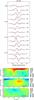 |
Fig. 5 Stokes V LSD profiles (upper panel) and the surface magnetic map (bottom panel) for observations of OU And gathered in 2008 with ℓ = 20. The plots follow the same definitions as in Figs. 2 and 3. |
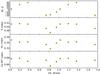 |
Fig. 6 Bl, S-index, Hα, Ca ii IR triplet indexes behavior for observations of OU And gathered in 2008. The plots follow the same definitions as in Fig. 1. |
To perform a more systematic comparison of the magnetic maps obtained five years apart, we cross-correlated every latitudinal band of the two maps following, for example, Petit et al. (2010), for each field component separately, which resulted in the three cross-correlation maps illustrated in Fig. 7. Using this approach, we highlight a strong correlation of both maps at all latitudes, provided that a ≈ 0.5 phase shift is applied. This correlation is easily visible by comparing the 2008 and 2013 maps with the naked eye, noticing that the maximal radial field value is observed at around phase 0.65 in 2008, and 0.15 in 2013. The lack of observations between 2008 and 2013 is obviously too large to decide whether this overall similarity is due to a global stability of the field geometry over this timespan, in which case the 0.5 phase shift between both maps would be compatible with our relatively large uncertainty on the stellar rotation period.
4.3. Magnetic mapping of 31 Com
According to the 6.8 d rotation period proposed by Strassmeier et al. (2010), the time series available for 31 Com is affected by a large phase gap, which spans about 40% of the rotation cycle, between phases 0.13 and 0.54. Given the relatively high inclination angle of the stellar spin axis (of the order of 80° when the rotation period, vsin(i) and radius are considered together, in the solid-body rotation hypothesis), this sparse phase coverage implies that a significant fraction of the theoretically accessible stellar surface remains completely unobserved for phases inside the gap and stellar latitudes below 80°. In spite of this well identified limitation, we decide to use our ten observations to reconstruct the large-scale magnetic geometry of its photosphere through ZDI.
Magnetic parameters.
For this we use vsin(i) = 67 km s-1 and i = 80°. Because of the relatively high vsin(i) value, we use a model with more spherical harmonics ℓmax = 20, to take full advantage of the higher spatial resolution offered by a larger projected rotational velocity. We also compute a ZDI model restricted to ℓmax = 10, to ease the comparison with our ZDI model of OU And. A set of ZDI models was computed for various values of the rotation period (between 2 d and 10 d), but the outcome does not reveal a preferred rotation period, presumably because of the poor phase coverage. A systematic search for latitudinal differential rotation was similarly unsuccessful. We therefore keep the period of Strassmeier et al. (2010) to compute the rotation phases, and assume solid-body rotation in the ZDI procedure.
The magnetic map resulting from the tomographic procedure with ℓmax = 20 is illustrated in Fig. 3 (right), while the fit to the observed Stokes V profiles is shown in Fig. 2. Magnetic quantities extracted from the maps are listed in Table 4. We achieve here  , showing that our model is able to reproduce the set of observational data close to the level of photon noise. The surface map displays a complex field geometry, with a majority (69%) of the poloidal magnetic energy stored in spherical harmonics modes with ℓ> 3. The surface magnetic energy is also equally distributed between the poloidal and toroidal field components. Owing to the high inclination angle, a majority of both stellar hemispheres can be observed. The apparent symmetry of the reconstructed magnetic geometry about the equator actually illustrates the difficulty of the tomographic code to distinguish between the hemispheres in this specific geometrical configuration. As expected with our sparse phase coverage, we note an absence of reconstructed magnetic regions between phase 0.2 and 0.5, owing to the lack of observational constraints at these phases. A likely consequence of this situation is that the average field strength reported in Table 4 may be underestimated by about 30%, because a large phase gap is hiding a significant fraction of the stellar surface and the maximum entropy reconstruction will force a null magnetic field in this unseen region.
Contrary to OU And for which maps with ℓmax = 10 and ℓmax = 20 can barely be distinguished (as illustrated by the numbers reported in Table 4), limiting the spherical harmonics expansion to ℓmax = 10 in our model of 31 Comae induces measurable modifications in the magnetic geometry. In particular, we observe that the surface smoothing imposed through ℓmax = 10 reduces the maximal field strength by about 7%, and increases by about 20% the amount of the magnetic energy reconstructed in modes with ℓ< 4.
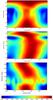 |
Fig. 7 Cross-correlation (2008 versus 2013) of magnetic maps of OU And derived for all three components of the magnetic vector with, from top to bottom, the radial, azimuthal, and meridional field projection. |
5. Evolutionary status
5.1. Stellar parameters
For OU And, Teff = 5850 K is inferred by Wright et al. (2003) from its spectral type. Gondoin (2003, 2005b) uses a cooler temperature (5110 K) but do not indicate how it was obtained. We then made our own determination of atmospheric parameters, as presented in Table 1, and used derived values in this work as well as in Aurière et al. (2015). We determined parameters of OU And, such as effective temperature (Teff), surface gravity (log g), microturbulence (ξ), and metallicity using the local thermodynamic equilibrium (LTE) model atmospheres of Kurucz (1993) and the current version of the spectral analysis code moog (Sneden 1973). We measured equivalent widths (EW) of 76 Fe i and 6 Fe ii lines in the spectrum obtained on September 25, 2008. The log gf values were taken from Lambert et al. (1996). The solution of the excitation equilibrium used to derive the effective temperature (Teff) was defined by a zero slope of the trend between the iron abundance derived from Fe i lines and the excitation potential of the measured lines. The microturbulent velocity (ξ) was found by constraining the abundance, determined from individual Fe i lines, to show no dependence on EWλ/λ. The value of log g was determined by means of the ionization balance assuming LTE. We then found Teff = 5360 K and log g = 2.80. Typical uncertainty in Teff and log g are ±120 K and ±0.2, respectively.
Using the above values for Teff, log g, and luminosity, the radius of the star is estimated to be R = 9.46 R⊙ assuming the bolometrical correction BC = −0.16 (Alonso et al. 1999) and the reddening AV = 0.09. The photometric period of OU And varies in different observational epochs. For magnetic field mapping, we adopted the value of 24.2 d that is close to the best fit of the ZDI models for 2008 and 2013 data, which was treated separately.
31 Comae is a member of the open cluster Mellote 111, also known as Coma Berenices Cluster (Casewell et al. 2006) and we may assume the metalicity and reddening follow those of the cluster. Mellote 111 has solar metalicity [Fe/H] = 0.00 ± 0.08 (Heiter et al. 2014) and its age is about 560 ± 90 Myr (Silaj & Landstreet 2014). Interstellar reddening in the direction of the Mellote 111 is E(B−V) = 0.00 (Robichon et al. 1999). Because of the very fast rotation of 31 Com, the lines in its spectrum are wide and blended and it is impossible to determine atmospheric parameters of this star in the same way as we did for OU And, measuring EWs of individual Fe i and Fe ii lines. For this reason we calculated a grid of synthetic spectra in a wide range of effective temperatures (Teff) in the spectral region 6080−6180 Å, which contains lines of neutral elements with different excitation potentials and lines of Fe ii, which are sensitive to surface gravity. Synthetic spectra calculated with Teff from 5550 K to 5700 K fit well the observed spectrum and it is difficult to obtain Teff with higher precision. Additionally, photospheric spots and active regions contribute to the strengthening or weakening of the lines of different elements. To derive the Teff value with higher precision, we used also photometric calibrations (see Table 5).
Photometric calibrations of the effective temperature of 31 Com.
We also found the following estimations of the effective temperature of 31 Com in the literature: 5689 K (Katz et al. 2011), 5747 K (Blackwell & Lynas-Gray 1998), 5761 K (Houdashelt et al. 2000), 5623 K (Massarotti 2008), and 5660 K (Strassmeier et al. 2010). Further in the paper we will use this latter value of the effective temperature (Teff = 5660 K), which we also used in Auriere et al. (2015). For radial velocity, rotation period, and vsin(i), we adopted the values derived by Strassmeier et al. (2010). We calculated the luminosity L = 73.4 L⊙ and stellar radius of R = 8.5 R⊙ using BC = −0.114 (Alonso et al. 1999) and E(B−V) = 0.00. Stellar mass M = 2.75 M⊙ and surface gravity log g = 2.97 are based on the evolutionary tracks discussed in the next section. Higher value of log g = 3.51 for 31 Comae, as suggested by Strassmeier et al. (2010), does not match our evolutionary models.
5.2. Evolutionary status, mass, and rotation
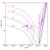 |
Fig. 8 Position of 31 Comae and OU And (circle and square, respectively) on the Hertzsprung-Russell diagram (HRD) diagram. Solar metallicity tracks of evolution models with different masses (indicated on the plot, in solar mass) are shown. The dashed black line delimits the beginning of the first dredge-up phase and corresponds with the evolution points when the mass of the convective envelope of the models encompasses 2.5% of the total stellar mass. The loops on the evolutionary tracks in the right part of the HRD (effective temperature below ~5000 K) correspond to the central helium-burning phase. |
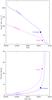 |
Fig. 9 Evolution of the surface rotation velocity (upper plot, in km s-1) and period (lower plot, in days) of the 2.7 and 2.85 M⊙ dedicated models for 31 Com and OU And (circle and square, respectively), compared with the observational data. |
The positions of OU And and 31 Com on the HR diagram are shown in Fig. 8. The values we use for the stellar effective temperatures are shown in Table 1 and section Sect. 5.1. Luminosity values are computed using the stellar parallaxes from the New Reduction Hipparcos catalogues by van Leeuwen (2007), the V magnitudes from the 1997 Hipparcos catalogue (ESA 1997), and applying the bolometric correction relation of Flower (1996).
The evolution tracks shown in Fig. 8 are for rotating models computed for solar metallicity with the code STAREVOL with the same input physics and assumptions as in Lagarde et al. (2012). For the 2.5 and 3.0 M⊙ models, the initial rotation velocity on the zero age main sequence Vzams corresponds to 30% of the critical velocity at that stage (Lagarde et al. 2014). For the present paper, we computed models of 2.7 and 2.85 M⊙ suited to 31 Com and OU And, respectively, with different Vzams to infer the initial rotation velocities of OU And and 31 Com. No magnetic braking is applied, and the rotation velocity of the models evolves mainly owing to structural changes of the star (in particular changes of stellar radius).
It is clear that both stars are in the Hertzsprung gap and have very similar masses of the order of ~2.7 and 2.85M⊙ for 31 Com and OU And, respectively, as already discussed in Aurière et al. (2015). Initial rotation velocities of 235 and 131 km s-1, which correspond respectively to 53 and 30% of the critical velocity on the ZAMS, are inferred to reproduce the present day rotation velocities and periods of 31 Com and OU And, respectively, as shown in Fig. 9.
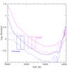 |
Fig. 10 Evolution of the theoretical Rossby number for the 2.7 and 2.85 M⊙ dedicated models (blue and magenta respectively). The full and dotted lines correspond to Rossby numbers computed with the turnover timescale taken, respectively, at half a pressure scale height above the base of the convective envelope and at its maximum value within the convective envelope. The rectangles correspond to the expected position of 31 Com and OU And, taking into account uncertainties in their effective temperatures. |
6. Discussion: origin of the magnetic field and activity of OU And and 31 Com
Figure 10 shows the evolution of the theoretical Rossby number for the 2.7 and 2.85 M⊙ models that fit the present-day rotation of 31 Comae and OU And (Sect. 5.2). RO is defined as the ratio between the rotational period and the convective turnover timescale, Prot/τc, and these quantities come directly from the stellar evolution computations. For each stellar mass we show cases when the Rossby number is computed using the turnover timescale at half a pressure scale height above the base of the convective envelope and at its maximum value within the convective envelope (full and dotted lines, respectively).
We see that the theoretical Rossby number decreases towards lower effective temperatures, owing to the fast increase of the convective turnover timescale as the convective envelope deepens in mass during the first dredge-up in the so-called magnetic strip (Charbonnel et al., in prep.).
Figure 10 shows that both stars have rather small Rossby number reaching about 0.5 at maximum value for τconv. This suggests that a dynamo-driven magnetic field could therefore be at work, which would be the origin of the large activity of these stars. However, these stars have significantly different rotation periods and magnetic field strengths. Better understanding of the magnetic activity of both stars gives the comparison of the magnetic field strength with the semi-emperical RO defined as the ratio between the observed Prot and the maximum value of the convective turnover timescale within the convective envelope. For OU And, the semi-emperical RO is 0.68 (Aurière et al. 2015), and it fits with our theoretical predictions. For 31 Comae it is 0.12, (Aurière et al. 2015), and it is about two times greater than our theoretical predictions. The faster rotator, 31 Com (Prot = 6.8 d) has magnetic field properties that are consistent with an α−ω dynamo-driven magnetic field (Aurière et al. 2015) and the magnetic map obtained in Sect. 4.3 is consistent with this hypothesis.
On the other hand, though OU And appears with a rather fast rotation period of 24.2 days, it is a deviating object on several plots presented in the study of Aurière et al. (2015), which led these authors to suppose that OU And is the probable descendant of a magnetic Ap star on the main sequence. Our ZDI study supports arguments to this hypothesis: its magnetic topology is mainly poloidal (82% of the magnetic energy in 2008) and the poloidal component is dominated by a dipole; furthermore, this topology appears to be quite stable. Figure 4 (right panel) illustrates the stability of the magnetic field from one rotation to the next one. A comparison of the maps obtained in 2008 (lower panel of Fig. 5) and in 2013 (left panel of Fig. 3) and the magnetic field parameters presented in Table 4 show that the magnetic topology is remarkably similar five years apart. Figure 11 also supports this statement and demonstrates that the 2008 Bl data, shifted with by half a cycle, overlap the rotational modulation of Bl in 2013. This might be an indication that the 0.5-cycle shift could be attributed to the precision of the period determination. However Table 4 shows that when the magnetic field strength increases between 2008 and 2013, the percentage strength of the poloidal component decreases from 82% to 64%, which corresponds to a correlated increase in the toroidal component. At the same time, the dipole contribution of the poloidal component remains the same. This indicates that the magnetic strength variation is mainly due to the toroidal component (probably of rotational dynamo origin), when the dipolar component (presumed to be of fossil origin) – remains about constant. This is consistent with our analysis that magnetic field of OU And is due to the interplay between convection and the remnant of the fossil field of an Ap star. Following the approach of Stepien (1993), with the assumption of magnetic flux conservation and a radius increase with stellar evolution to the red-giant branch (RGB), we can infer the dipole strength of a possible Ap star progenitor of OU And. Having a radius on the Main Sequence (MS) of 2.2 R⊙, obtained by the proposed evolutionary model and the mean and maximum poloidal component of the magnetic field strength in 2013 (Table 4), we find the initial values for magnetic dipole strength on the main sequence of the HRD of about 800 to 4600 G, respectively, consistent with values for Ap stars. The predicted rotation of OU And on the MS, with vsin(i) of about 100 km s-1 (assuming i = 50°), is faster than the mean for Ap stars but is still consistent with the Ap star status. Very few Ap stars are known to have fast rotation (vsin(i) over 100 km s-1), but this type of small sample does exist, according to Wraight et al. (2012).
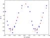 |
Fig. 11 Bl of OU And in 2013 (circles) and in 2008 shifted with 0.5 cycle (triangles). |
Direct comparison of the properties of OU And and 31 Com emphasizes the differences that were listed just above. Both stars have about the same mass, about the same evolutionary state, and the same order of high level X-ray activity. Though 31 Com rotates three times faster than OU And, the magnetic strength of OU And is twice that of 31 Com. Figures 2 and 3 clearly show the difference in magnetic topology: a large scale dominant structure for OU And, a smaller scale dominant structure for 31 Com. While the magnetic map of 31 Com can be compared to that of 390 Aur (Konstantinova-Antova et al. 2012), the outstandingly strong large scale magnetic field of OU And is reminiscent of the properties observed on EK Eri, which is the archetype of the descendants of magnetic Ap stars on the main sequence (Stepien 1993; Strassmeier et al. 1999; Aurière et al. 2008, 2012). We also need to mention that the dynamo models, suitable for some M dwarfs and capable of producing fields like the one for OU And, are not effective in this case, because M dwarfs have huge convective zones or are fully convective for spectral types that are cooler than M3 (Morin et al. 2010). On the other hand, in the case of intermediate mass stars in the Hertzsprung gap, the convective envelope is just beginning to develop and a possible dynamo mechanism starts to work. If a toroidal field at the surface of the star is detected, this is a strong indication of a distributed dynamo (Donati et al. 2003). A dynamo-generated magnetic field at this evolutionary stage could be produced in a fast rotator by a dynamo mechanism (the case of 31 Comae), as well as from the Ap star fossil magnetic field interacting with relatively fast remnant rotation. Without a remnant Ap magnetic field, OU And with its rotational rate should be less active and with a weaker magnetic field than 31 Comae.
7. Conclusions
It is well known that intermediate mass stars on the MS do not have a convective envelope as well as nor do they have dynamo-driven surface magnetic fields and winds that carry away angular momentum and slow down the rotation. A recently published paper (Stello et al. 2016) demonstrates that most MS intermediate mass stars host a strong dynamo in their core, the product of this dynamo being confined deep in the star and, consequently, does not show at surface level.
On the other hand, we have studied the case of two evolved intermediate stars with magnetic activity and, for the first time, performed the ZDI magnetic mapping of OU And and 31 Com. Thanks to dedicated evolutionary models, including rotation (Charbonnel & Lagarde 2010), we can precise the evolutionary status of these stars in the Hertzsprung gap and the history of their rotation, which has not been affected by magnetic braking, neither on the main sequence nor after, hence magnetic braking plays no role until the star develops a cool star structure.
Observational properties of red giants, i.e., fast rotators with dynamo magnetic fields are: a Rossby number smaller than unity, peaks and bumps in the Stokes I profile, a complex structure in the magnetic map and a significant toroidal component of the MF. Depending on the thickness of the convective envelope and rotational rate in some stars, we also can observe an azimuthal belt in the magnetic map (e.g., V390 Aur, Konstantinova-Antova et al. 2012). There is also a dependence of the magnetic field strength on rotation (Konstantinova-Antova et al. 2013; Aurière et al. 2015), which is clear evidence of an α-ω dynamo operation.
Both the individual analysis of the magnetic fied and activity of each star and a direct comparison of their properties show that they illustrate the evolution of a fast rotator on the one hand (31 Com), and of a probable Ap star descendant (OU And), on the other. The origin of the magnetic field at the surface of 31 Com is suspected to be dynamo-driven. The dipolar magnetic field component of OU And could be the remnant of of an Ap star on the main sequence, now interacting with convection. The toroidal magnetic field component of OU And may be due to a dynamo as a result of the fast rotation of the star. The two stars are observed as being still at the beginning of their evolution off the main sequence: the convective envelope of 31 Com is still rather shallow and the magnetic dipole strength from the Ap star progenitor of OU And is diluted by about 18 times. In its present evolutionary state, the magnetic field of OU And is significantly stronger than that of 31 Com, as it is for for the Ca ii H&K and Hα lines, too. The two stars are more similar for their Lx and the strength of other activity indicators. In the sample studied by Aurière et al. (2015), only one star of similar mass (3 M⊙), ι Cap, has such a high rotaional rate with measured Prot (68 d). This is located at the base of the RGB, and it does not deviate from the mean relation between rotation and magnetic field strength observed by Aurière et al. (2015): its magnetic field is likely to be dynamo-driven and may illustrate the changes of rotational and magnetic field properties expected for 31 Com when reaching the same evolutionary status. The | Bl | max of ι Cap is of 8.3 G, which is about the same as for 31 Com in its present state in the Hertzsprung gap. This may indicate that, at the evolutionary state of ι Cap (at the base of the RGB) when the convective envelope deepens and the convective turnover time increases but the rotation rate decreases (because of magnetic braking and increased radius) the magnetic field strength produced by the dynamo of 31 Comae will remain of the same magnitude. However, at the same evolutionary stage, using the models presented in Aurière et al. (2015) and the hypothesis for magnetic flux conservation, the magnetic strength of the dipole of OU And only drops by a factor of 2, and is still significantly stronger than the magnetic strength of 31 Com. These extrapolations suggest that the Ap-star descendants, even with moderate magnetic dipoles like OU And, will remain outstanding objects with respect to the period/magnetic strength relation up until they begin ascend the RGB.
Acknowledgments
We are thankful to the TBL team for providing service observations with Narval spectropolarimeter. Observations in 2013 were funded under the project BG051PO001-3.3.06-0047 financed by the EU, ESF, and Republic of Bulgaria. Observations in 2008 were funded under an OPTICON project. This work was also supported by the Bulgarian NSF contracts DRILA 01/03 and DMU 03-87. N.A.D. thanks Saint Petersburg State University, Russia, for research grant 6.38.18.2014 and FAPERJ, Rio de Janeiro, Brazil, for visiting researcher grant E-26/200.128/2015. The authors gratefully acknowledge the constructive comments and input offered by the referee.
References
- Alonso, A., Arribas, S., & Martínez-Roger, C. 1999, A&AS, 140, 261 [NASA ADS] [CrossRef] [EDP Sciences] [Google Scholar]
- Aurière, M., Konstantinova-Antova, R., Petit, P., et al. 2008, A&A, 491, 499 [NASA ADS] [CrossRef] [EDP Sciences] [Google Scholar]
- Aurière, M., Konstantinova-Antova, R., Petit, P., et al. 2011, A&A, 534, A139 [NASA ADS] [CrossRef] [EDP Sciences] [Google Scholar]
- Aurière, M., Konstantinova-Antova, R., Petit, P., et al. 2012, A&A, 543, A118 [NASA ADS] [CrossRef] [EDP Sciences] [Google Scholar]
- Aurière, M., Konstantinova-Antova, R., Charbonnel, C., et al. 2015, A&A, 574, A90 [NASA ADS] [CrossRef] [EDP Sciences] [Google Scholar]
- Ayres, T. R., Simon, T., Stern, R. A., et al. 1998, ApJ, 496, 428 [NASA ADS] [CrossRef] [Google Scholar]
- Ayres, T. R., Hodges-Kluck, E., & Brown, A. 2007, ApJS, 171, 304 [NASA ADS] [CrossRef] [Google Scholar]
- Blackwell, D. E., & Lynas-Gray, A. E. 1998, A&AS, 129, 505 [NASA ADS] [CrossRef] [EDP Sciences] [Google Scholar]
- Casewell, S. L., Jameson, R. F., & Dobbie, P. D. 2006, MNRAS, 365, 447 [NASA ADS] [CrossRef] [Google Scholar]
- Charbonnel, C., & Lagarde, N. 2010, A&A, 522, A10 [NASA ADS] [CrossRef] [EDP Sciences] [MathSciNet] [PubMed] [Google Scholar]
- Charbonnel, C., Decressin, T., Lagarde, N., et al. 2016, A&A, in press [Google Scholar]
- Cowley, A. P., & Bidelman, W. P. 1979, PASP, 91, 83 [NASA ADS] [CrossRef] [Google Scholar]
- de Medeiros, J. R., & Mayor, M. 1999, A&AS, 139, 433 [NASA ADS] [CrossRef] [EDP Sciences] [Google Scholar]
- Donati, J.-F. 2001, in Astrotomography, Indirect Imaging Methods in Observational Astronomy, eds. H. M. J. Boffin, D. Steeghs, & J. Cuypers (Berlin: Springer Verlag), Lect. Notes Phys., 573, 207 [Google Scholar]
- Donati, J.-F., & Brown, S. F. 1997, A&A, 326, 1135 [NASA ADS] [Google Scholar]
- Donati, J.-F., Brown, S. F., Semel, M., et al. 1992, A&A, 265, 682 [NASA ADS] [Google Scholar]
- Donati, J.-F., Semel, M., Carter, B. D., Rees, D. E., & Collier Cameron, A. 1997, MNRAS, 291, 658 [NASA ADS] [CrossRef] [MathSciNet] [Google Scholar]
- Donati, J.-F., Collier Cameron, A., Semel, M., et al. 2003, MNRAS, 345, 1145 [NASA ADS] [CrossRef] [Google Scholar]
- Donati, J.-F., Catala, C., Landstreet, J. D., & Petit, P. 2006a, in ASP Conf. Ser. 358, eds. R. Casini, & B. W. Lites, 362 [Google Scholar]
- Donati, J.-F., Howarth, I. D., Jardine, M. M., et al. 2006b, MNRAS, 370, 629 [NASA ADS] [CrossRef] [Google Scholar]
- Ducati, J. R. 2002, VizieR Online Data Catalog: II/237 [Google Scholar]
- Duncan, D. K., Vaughan, A. H., Wilson, O. C., et al. 1991, ApJS, 76, 383 [NASA ADS] [CrossRef] [Google Scholar]
- ESA 1997, VizieR Online Data Catalog: I/239 [Google Scholar]
- Flower, P. J. 1996, ApJ, 469, 355 [NASA ADS] [CrossRef] [Google Scholar]
- Gizis, J. E., Reid, I. N., & Hawley, S. L. 2002, AJ, 123, 3356 [NASA ADS] [CrossRef] [Google Scholar]
- Gondoin, P. 1999, A&A, 352, 217 [NASA ADS] [Google Scholar]
- Gondoin, P. 2003, A&A, 409, 263 [NASA ADS] [CrossRef] [EDP Sciences] [Google Scholar]
- Gondoin, P. 2005a, A&A, 444, 531 [NASA ADS] [CrossRef] [EDP Sciences] [Google Scholar]
- Gondoin, P. 2005b, in 13th Cambridge Workshop on Cool Stars, Stellar Systems and the Sun, eds. F. Favata, G. A. J. Hussain, & B. Battrick, ESA SP, 560, 587 [Google Scholar]
- González Hernández, J. I., & Bonifacio, P. 2009, A&A, 497, 497 [NASA ADS] [CrossRef] [EDP Sciences] [Google Scholar]
- Gray, R. O., Napier, M. G., & Winkler, L. I. 2001, AJ, 121, 2148 [NASA ADS] [CrossRef] [Google Scholar]
- Hauck, B., & Mermilliod, M. 1998, A&AS, 129, 431 [NASA ADS] [CrossRef] [EDP Sciences] [Google Scholar]
- Heiter, U., Soubiran, C., Netopil, M., & Paunzen, E. 2014, A&A, 561, A93 [NASA ADS] [CrossRef] [EDP Sciences] [Google Scholar]
- Hopkins, J. L., Boyd, L. J., Genet, R. M., & Hall, D. S. 1985, Information Bulletin on Variable Stars, 2684, 1 [NASA ADS] [Google Scholar]
- Houdashelt, M. L., Bell, R. A., & Sweigart, A. V. 2000, AJ, 119, 1448 [Google Scholar]
- Katz, D., Soubiran, C., Cayrel, R., et al. 2011, A&A, 525, A90 [NASA ADS] [CrossRef] [EDP Sciences] [Google Scholar]
- Kochukhov, O., Makaganiuk, V., & Piskunov, N. 2010, A&A, 524, A5 [NASA ADS] [CrossRef] [EDP Sciences] [Google Scholar]
- Konstantinova-Antova, R., Aurière, M., Petit, P., et al. 2012, A&A, 541, A44 [NASA ADS] [CrossRef] [EDP Sciences] [Google Scholar]
- Konstantinova-Antova, R., Auríere, M., Charbonnel, C., et al. 2013, Bulgarian Astron. J., 19, 14 [Google Scholar]
- Konstantinova-Antova, R., Aurière, M., Charbonnel, C., et al. 2014, in IAU Symp., 302, 373 [Google Scholar]
- Kupka, F. G., Ryabchikova, T. A., Piskunov, N. E., Stempels, H. C., & Weiss, W. W. 2000, Balt. Astron., 9, 590 [NASA ADS] [Google Scholar]
- Kurucz, R. 1993, SYNTHE Spectrum Synthesis Programs and Line Data, Kurucz CD-ROM No. 18 (Cambridge, Mass.: Smithsonian Astrophysical Observatory) [Google Scholar]
- Lagarde, N., Decressin, T., Charbonnel, C., et al. 2012, A&A, 543, A108 [NASA ADS] [CrossRef] [EDP Sciences] [Google Scholar]
- Lagarde, N., Anderson, R. I., Charbonnel, C., et al. 2014, A&A, 570, C2 [NASA ADS] [CrossRef] [EDP Sciences] [Google Scholar]
- Lambert, D. L., Heath, J. E., Lemke, M., & Drake, J. 1996, ApJS, 103, 183 [NASA ADS] [CrossRef] [Google Scholar]
- Marsden, S. C., Petit, P., Jeffers, S. V., et al. 2014, MNRAS, 444, 3517 [NASA ADS] [CrossRef] [Google Scholar]
- Massarotti, A. 2008, AJ, 135, 2287 [NASA ADS] [CrossRef] [Google Scholar]
- Morin, J., Donati, J.-F., Petit, P., et al. 2010, MNRAS, 407, 2269 [NASA ADS] [CrossRef] [MathSciNet] [Google Scholar]
- Petit, P., Donati, J.-F., & Collier Cameron, A. 2002, MNRAS, 334, 374 [NASA ADS] [CrossRef] [MathSciNet] [Google Scholar]
- Petit, P., Lignières, F., Wade, G. A., et al. 2010, A&A, 523, A41 [NASA ADS] [CrossRef] [EDP Sciences] [Google Scholar]
- Petit, P., Aurière, M., Konstantinova-Antova, R., et al. 2013, in Lect. Notes Phys. 857, eds. J.-P. Rozelot, & C. Neiner (Berlin: Springer Verlag), 231 [Google Scholar]
- Rees, D. E., & Semel, M. D. 1979, A&A, 74, 1 [NASA ADS] [Google Scholar]
- Robichon, N., Arenou, F., Mermilliod, J.-C., & Turon, C. 1999, A&A, 345, 471 [NASA ADS] [Google Scholar]
- Semel, M. 1989, A&A, 225, 456 [NASA ADS] [Google Scholar]
- Silaj, J., & Landstreet, J. D. 2014, VizieR Online Data Catalog: J/A+A/566/A132 [Google Scholar]
- Skrutskie, M. F., Cutri, R. M., Stiening, R., et al. 2006, AJ, 131, 1163 [NASA ADS] [CrossRef] [Google Scholar]
- Sneden, C. 1973, ApJ, 184, 839 [NASA ADS] [CrossRef] [Google Scholar]
- Stello, D., Cantiello, M., Fuller, J., et al. 2016, Nature, 529, 364 [NASA ADS] [CrossRef] [PubMed] [Google Scholar]
- Stepien, K. 1993, ApJ, 416, 368 [NASA ADS] [CrossRef] [Google Scholar]
- Strassmeier, K. G., & Hall, D. S. 1988, ApJS, 67, 453 [NASA ADS] [CrossRef] [Google Scholar]
- Strassmeier, K. G., Serkowitsch, E., & Granzer, T. 1999, A&AS, 140, 29 [NASA ADS] [CrossRef] [EDP Sciences] [Google Scholar]
- Strassmeier, K. G., Granzer, T., Kopf, M., et al. 2010, A&A, 520, A52 [NASA ADS] [CrossRef] [EDP Sciences] [Google Scholar]
- Tsvetkova, S., Petit, P., Aurière, M., et al. 2013, A&A, 556, A43 [Google Scholar]
- van Leeuwen, F. 2007, A&A, 474, 653 [NASA ADS] [CrossRef] [EDP Sciences] [Google Scholar]
- Wade, G. A., Donati, J.-F., Landstreet, J. D., & Shorlin, S. L. S. 2000, MNRAS, 313, 823 [NASA ADS] [CrossRef] [MathSciNet] [Google Scholar]
- Wraight, K. T., Fossati, L., Netopil, M., et al. 2012, MNRAS, 420, 757 [NASA ADS] [CrossRef] [Google Scholar]
- Wright, C. O., Egan, M. P., Kraemer, K. E., & Price, S. D. 2003, AJ, 125, 359 [NASA ADS] [CrossRef] [Google Scholar]
Appendix A: Determining the atmospheric parameters of OU And
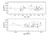 |
Fig. A.1 Abundance of Fe i lines versus excitation potential. The correct temperature is indicated by a zero slope in this plot. Bottom: abundance of Fe i lines versus showing determination of the microturbulent velocity. |
Fe i and Fe ii lines used for atmospheric parameter determination.
All Tables
Spectropolarimetric observations, activity indicators and Bl measurements for 31 Com in 2013.
All Figures
|
Fig. 1 Bl, S-index, Hα, and Ca ii IR triplet indexes behavior for OU And (left) and 31 Com (right). For both stars, phases are computed for ephemeris HJD0 = 2 454 101.5 and the rotational period of 24.2 d for OU And and 6.8 d for 31 Com. |
| In the text | |
|
Fig. 2 Observed Stokes V LSD profiles (black line) and profiles produced by our best ZDI model (red lines) for OU And (left) and 31 Comae (right). Successive profiles are vertically shifted (from top to bottom) for display clarity. The rotational phase of each observation (computed from the ephemeris given in the text) is listed to the right, with the integer part denoting the rotational cycle since the start of the observing run. Error bars are illustrated on the left of every profile and dashed lines illustrate the zero level. |
| In the text | |
|
Fig. 3 Photospheric magnetic maps of OU And (left) and 31 Com (right) in 2013. For each star, the vectorial magnetic field is split in its three components in spherical projection and ℓmax = 20. The color scale illustrates the field strength in Gauss, and the rotational phases of our data sets show up as vertical ticks on top of each map. |
| In the text | |
|
Fig. 4 Evolution of Stokes I and Stokes V (left and right, respectively) LSD profiles of OU And observed close to phase 0.4. We represent in black the observation of 2013 Sept. 19 (phase 0.41) and in red the observation of 2013 Oct. 13 (phase 0.40). |
| In the text | |
|
Fig. 5 Stokes V LSD profiles (upper panel) and the surface magnetic map (bottom panel) for observations of OU And gathered in 2008 with ℓ = 20. The plots follow the same definitions as in Figs. 2 and 3. |
| In the text | |
|
Fig. 6 Bl, S-index, Hα, Ca ii IR triplet indexes behavior for observations of OU And gathered in 2008. The plots follow the same definitions as in Fig. 1. |
| In the text | |
|
Fig. 7 Cross-correlation (2008 versus 2013) of magnetic maps of OU And derived for all three components of the magnetic vector with, from top to bottom, the radial, azimuthal, and meridional field projection. |
| In the text | |
|
Fig. 8 Position of 31 Comae and OU And (circle and square, respectively) on the Hertzsprung-Russell diagram (HRD) diagram. Solar metallicity tracks of evolution models with different masses (indicated on the plot, in solar mass) are shown. The dashed black line delimits the beginning of the first dredge-up phase and corresponds with the evolution points when the mass of the convective envelope of the models encompasses 2.5% of the total stellar mass. The loops on the evolutionary tracks in the right part of the HRD (effective temperature below ~5000 K) correspond to the central helium-burning phase. |
| In the text | |
|
Fig. 9 Evolution of the surface rotation velocity (upper plot, in km s-1) and period (lower plot, in days) of the 2.7 and 2.85 M⊙ dedicated models for 31 Com and OU And (circle and square, respectively), compared with the observational data. |
| In the text | |
|
Fig. 10 Evolution of the theoretical Rossby number for the 2.7 and 2.85 M⊙ dedicated models (blue and magenta respectively). The full and dotted lines correspond to Rossby numbers computed with the turnover timescale taken, respectively, at half a pressure scale height above the base of the convective envelope and at its maximum value within the convective envelope. The rectangles correspond to the expected position of 31 Com and OU And, taking into account uncertainties in their effective temperatures. |
| In the text | |
|
Fig. 11 Bl of OU And in 2013 (circles) and in 2008 shifted with 0.5 cycle (triangles). |
| In the text | |
|
Fig. A.1 Abundance of Fe i lines versus excitation potential. The correct temperature is indicated by a zero slope in this plot. Bottom: abundance of Fe i lines versus showing determination of the microturbulent velocity. |
| In the text | |
Current usage metrics show cumulative count of Article Views (full-text article views including HTML views, PDF and ePub downloads, according to the available data) and Abstracts Views on Vision4Press platform.
Data correspond to usage on the plateform after 2015. The current usage metrics is available 48-96 hours after online publication and is updated daily on week days.
Initial download of the metrics may take a while.