| Issue |
A&A
Volume 590, June 2016
|
|
|---|---|---|
| Article Number | A72 | |
| Number of page(s) | 11 | |
| Section | Interstellar and circumstellar matter | |
| DOI | https://doi.org/10.1051/0004-6361/201527064 | |
| Published online | 13 May 2016 | |
The initial conditions for stellar protocluster formation
III. The Herschel counterparts of the Spitzer Dark Cloud catalogue⋆
1
School of Physics & Astronomy, Cardiff University,
Queen’s building, The parade,
Cardiff
CF24 3AA,
UK
e-mail:
This email address is being protected from spambots. You need JavaScript enabled to view it.
2
Jodrell Bank Centre for Astrophysics, Alan Turing building, School
of Physics & Astronomy, The University of Manchester,
Oxford Road, Manchester
M13 9PL,
UK
3
IAPS-Istituto di Astrofisica e Planetologia Spaziali, via Fosso
del Cavaliere 100, 00133
Roma,
Italy
4
Centre for Astrophysics Research, University of
Hertfordshire, College Lane,
Hatfield, Herts
AL10 9AB,
UK
5
Jeremiah Horrocks Institute, University of Central
Lancashire, Preston, Lancashire
PR1 2HE,
UK
Received: 27 July 2015
Accepted: 5 February 2016
Abstract
Context. Galactic plane surveys of pristine molecular clouds are key for establishing a Galactic-scale view of star formation. For this reason, an unbiased sample of infrared dark clouds in the 10° < | l | < 65°, | b | < 1° region of the Galactic plane was built using Spitzer 8 μm extinction. However, intrinsic fluctuations in the mid-infrared background can be misinterpreted as foreground clouds.
Aims. The main goal of this study is to disentangle real clouds in the Spitzer Dark Cloud (SDC) catalogue from artefacts due to fluctuations in the mid-infrared background.
Methods. We constructed H2 column density maps at ~18″ resolution using the 160 μm and 250 μm data from the Herschel Galactic plane survey Hi-GAL. We also developed an automated detection scheme that confirms the existence of a SDC through its association with a peak on these Herschel column density maps. Detection simulations, along with visual inspection of a small sub-sample of SDCs, have been performed to get more insight into the limitations of our automated identification scheme.
Results. Our analysis shows that 76( ± 19)% of the catalogued SDCs are real. This fraction drops to 55( ± 12)% for clouds with angular diameters larger than ~1 arcmin. The contamination of the PF09 catalogue by large spurious sources reflects the large uncertainties associated to the construction of the 8 μm background emission, a key stage in identiying SDCs. A comparison of the Herschel confirmed SDC sample with the BGPS and ATLASGAL samples shows that SDCs probe a unique range of cloud properties, reaching down to more compact and lower column density clouds than any of these two (sub-)millimetre Galactic plane surveys.
Conclusions. Even though about half of the large SDCs are spurious sources, the vast majority of the catalogued SDCs do have a Herschel counterpart. The Herschel-confirmed sample of SDCs offers a unique opportunity to study the earliest stages of both low- and high-mass star formation across the Galaxy.
Key words: catalogs / stars: formation / ISM: clouds / dust, extinction
Full Table 1 is only available at the CDS via anonymous ftp to cdsarc.u-strasbg.fr (130.79.128.5) or via http://cdsarc.u-strasbg.fr/viz-bin/qcat?J/A+A/590/A72
© ESO, 2016
 |
Fig. 1 Images of SDC324.633+0.779. From left to right: Spitzer 8 μm image with the τ8 μm = 0.35 opacity contour showing the boundary of the SDC as defined in PF09; Herschel H2 column density map with background; Herschel background filtered H2 column density map; Herschel dust temperature map. |
1. Introduction
Only in recent years have technological breakthroughs made far-infrared/sub-millimetre Galactic plane surveys at sub-arcminute resolution possible (Schuller et al. 2009; Molinari et al. 2010; Aguirre et al. 2011). These surveys have, for the first time, the sensitivity and resolution to probe the individual dust clumps in which stars form, providing a high-resolution view of the star formation process on a Galactic scale. In particular, a complete understanding of the origin and distribution of stellar masses is only possible with large surveys of clumps that sample the full range of different physical properties and in which the initial conditions for star formation are still imprinted. In this context, performing a Galactic plane survey of infrared dark clouds (IRDCs) is essential.
IRDCs were first observed in 1996 by Perault et al. using ISOCAM at 15 μm as absorption features against the infrared background of the Galactic plane. Since then, follow-up observations have shown that these sources are cold, dense molecular clouds and potential mass reservoirs for future generations of stars (e.g. Teyssier et al. 2002; Simon et al. 2006; Rathborne et al. 2006; Ragan et al. 2009). Their darkness in the mid-infrared domain ensures that these sources represent early stages in dense cloud evolution and, as such, IRDCs might contain the initial conditions of star formation. Peretto & Fuller (2009, Paper I, hereafter PF09) constructed a catalogue of over 11 000 Spitzer dark clouds (SDCs) using the 8 μm GLIMPSE Galactic plane survey (Churchwell et al. 2009) covering the 10°< | l | < 65°, | b | < 1° region (see Fig. 1 for an example of a SDC). In PF09, 4′′ angular resolution column density maps were constructed from the 8 μm extinction for all SDCs. This database has been used since for follow-up observations of specific clouds (Peretto et al. 2010, 2013, 2014), but also to tackle Galactic-scale problematics, such as the mass distribution of IRDCs and their sub-structures (Peretto & Fuller 2010), the existence of column density thresholds for the formation of massive stars (Kauffmann & Pillai 2010), or the characterisation of massive dense clumps (Traficante et al. 2015). This type of global study is the main reason behind building the PF09 catalogue in the first place. However, the PF09 catalogue is contaminated by spurious clouds since any significant dip in the 8 μm emission of the Galactic plane on angular scales lower than ~5′ is considered to be the result of the extinction by a cloud, while it could simply be due to the intrinsic variation of the Galactic plane emission. Disentangling between real and spurious SDCs is therefore crucial for any Galactic-scale study that makes use of the PF09 catalogue.
Wilcock et al. (2012) looked at the 300° <l< 330° region of the Galactic plane using Herschel Hi-GAL data and visually estimated that only 38% of the dark clouds from the PF09 catalogue were bright at 250 μm. Taken at face value, this suggests that most of the catalogued SDCs are artefacts, with only a minority of them real, casting doubt on any global-scale study that is based on the entire PF09 catalogue. However, a more rigorous approach to cloud identification is to systematically assess which SDCs are associated with peaks in the H2 column density determined from Hi-GAL data. This is the main objective of the present study.
In this paper, we present an analysis of the Herschel counterparts of all SDCs from the PF09 catalogue based on H2 column density images. Section 2 presents the observations. Section 3 describes how Herschel column density maps are constructed. Section 4 explains the identification scheme and its limitations. Section 5 presents a comparison between the automated and visual detection fractions of SDCs. In Sect. 6 we investigate the percentage of real SDCs that are detected in recent (sub-)millimetre Galactic plane surveys. Finally, summary and conclusions are in Sect. 7.
2. Herschel data
To confirm the nature of the SDCs, we use far-infrared dust emission data taken with the Herschel Space Observatory (Pilbratt et al. 2010). The two onboard photometry instruments, PACS (Poglitsch et al. 2010) and SPIRE (Griffin et al. 2010), allow the simultaneous observation of the dust emission at five wavelengths in the range 70−500 μm. The Hi-GAL open-time key project (Molinari et al. 2010) has observed the entire Galactic plane for a Galactic latitude | b | < 1° at wavelengths of 70, 160, 250, 350, and 500 μm, offering a unique opportunity to study the dust emission properties of SDCs.
The Hi-GAL data were reduced, as described in Traficante et al. (2011), using HIPE (Ott 2010) for calibration and deglitching (SPIRE only), routines especially developed for Hi-GAL data reduction (drift removal, deglitching), and the ROMAGAL map-making algorithm. Post-processing on the maps was applied to help with image artefact removal (Piazzo et al. 2015). In this paper, we make use of only the PACS 160 μm and SPIRE 250 μm data with a nominal angular resolution of θ160 = 12′′ and θ250 = 18′′, respectively.
In addition, zero-flux levels for every Hi-GAL field have been recovered by correlating Herschel data with Planck and IRAS data (Bernard et al. 2010).
3. Column density from Herschel
The main goal of this study is to disentangle real from spurious SDCs in the PF09 catalogue. We believe that Herschel column density maps are probably the most suitable data to do so. In this section, we discuss the construction and reliability of our Herschel column density maps.
3.1. Building 18′′Herschel column density maps from the 160 μm/250 μm colour
A difference in angular resolution is a major issue when cross-correlating two samples of sources. For this reason, it is essential here that we construct the highest possible angular resolution column density maps using the Herschel data. The typical way to construct Herschel column density maps is to perform pixel-by-pixel SED fitting using Herschel data at four or five wavelengths (e.g. Peretto et al. 2010; Battersby et al. 2011). While this is the most reliable way of constructing such maps, it requires the data to be smoothed to the resolution at the longest wavelength, i.e. ~36″ at 500 μm. For the purpose of confirming whether a SDC corresponds to a column density peak, a simpler, faster analysis can be used, one that also produces higher angular resolution column density maps.
Here we use the ratio of the Hi-GAL 160 μm over 250 μm images as a temperature tracer, and use the derived temperature to estimate the column density from the 250 μm data. The 160 μm-to-250 μm flux ratio, R160/250, can be written as  (1)where Sλ is the flux density at the wavelength λ, Bν is the Planck function, Td the dust temperature, and β the spectral index of the specific dust opacity law set to 2 (Hildebrand 1983). As shown in Fig. 2, R160/250 is a monotonic function of the dust temperature, so it can be used to estimate the dust temperature. In the 10−20 K temperature range, which is typical of IRDCs (Peretto et al. 2010), this ratio varies by a factor of ~5. In practice, because the 160 μm and 250 μm images originally have different pixels sizes and projection centres, we regridded the 160 μm images to match the 250 μm image astrometry. We then convolved the 160 μm images to the 250 μm image resolution using a Gaussian kernel of FWHM
  ′′. We used the resulting convolved 160 μm image with the original 250 μm image to compute the R160/250 ratio maps. We then converted the Hi-GAL R160/250 maps into a temperature map. The signal-to-noise ratio in Hi-GAL maps is very high with a minimum value of 10 at 160 and 250 μm for the faintest regions of the Galactic plane covered by Herschel (Molinari et al. 2016). This means that for the vast majority of the SDCs studied here, the uncertainty on R160/250 is only a few percent, which translates into a temperature uncertainty of a few tenths of a Kelvin. To calculate the column density map, we then combine this temperature map with the Hi-GAL 250 μm image, to derive the column density through the equation:
 ![Mathematical equation: \begin{equation} \label{eq_coldens} N_{{\rm H}_2} = S_{250}/[B_{\nu_{250}} (T_{\rm d})\kappa_{250} ~\mu {\rm m}_{\rm H}] \end{equation}](/articles/aa/full_html/2016/06/aa27064-15/aa27064-15-eq28.png) (2)where κ250 = 0.12 cm2 g-1 (Ossenkopf & Henning 1994) is the specific dust opacity at 250 μm (that already includes a dust-to-gas mass ratio of 1%), μ = 2.33 is average molecular weight, and mH the atomic mass of hydrogen. The simplicity of this method allows rapid construction of relatively high (i.e. 18′′) angular resolution column density maps for all the SDCs (see Fig. 1).
(2)where κ250 = 0.12 cm2 g-1 (Ossenkopf & Henning 1994) is the specific dust opacity at 250 μm (that already includes a dust-to-gas mass ratio of 1%), μ = 2.33 is average molecular weight, and mH the atomic mass of hydrogen. The simplicity of this method allows rapid construction of relatively high (i.e. 18′′) angular resolution column density maps for all the SDCs (see Fig. 1).
 |
Fig. 2 Variation in R160/250, the ratio between 160 μm to 250 μm flux density as a function of dust temperature (see Eq. (1)). A value of 2 was adopted for the spectral index of the dust opacity law (i.e. β). |
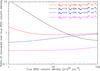 |
Fig. 3 Uncertainty linked to our column density construction method. In this plot we show the input IRDC column density versus the ratio of the retrieved column density versus true IRDC column density. The different colours correspond to different background properties. |
The column density we measure towards an IRDC is integrated along the line of sight and is the sum of the dust column density from the IRDC and the warmer column density from the background. These two components have potentially different dust properties (temperature and specific opacities) and column densities. In some places, the background column density can be higher than the column density of the cloud itself. It is possible to reconstruct the background first and remove its contribution to the observed fluxed towards the IRDCs (Peretto et al. 2010; Battersby et al. 2011). However, this is a difficult task for such a large sample of objects. For this reason, we decided to use a more practical method that filters out large scale structures in the column density map constructed as described above. For this purpose we used a 10′ wide median filter on the Herschel column density maps to create a background image, and subtracted this median component from the original column density image to create a background-subtracted column density map (see Fig. 1). These are the maps that we used for the rest of the analysis. The width of the filter was chosen so that it has a similar size to the largest SDCs in the catalogue.
3.2. The impact of background and SDC dust emission mixing on retrieved cloud properties
Estimating the column density without separating the background and IRDC contributions to the flux densities could lead to errors on the retrieved column density and temperature of IRDCs. To quantify this error, we modelled the emission of a background and IRDC components as modified-blackbodies at different temperatures and column densities, and added their respective flux densities at both 160 μm and 250 μm. We then used the same procedure as outlined in the previous section to estimate the temperature and column density of the combined IRDC/background components. We finally removed the original background column density from the combined column density to retrieve the IRDC column density. We varied both the properties (column density and dust emissivity index) of the background and the column density of the IRDC itself (with a constant temperature of 12 K). In Fig. 3 we show the ratio of the recovered IRDC column density using this technique over the input IRDC column density for different background/IRDC properties. One can see that the errors on the IRDC column densities can be quite high (up to a factor of 10 for low column density IRDCs) for warm and high-column density backgrounds. However, for more typical background properties, the errors are within a factor of 2. In all cases, the temperature of the IRDC is overestimated by only a few tenths of a Kelvin in the best cases and up to 10 K in the most difficult cases (low-column density IRDCs against high-column density and warm background).
 |
Fig. 4 Ratio of the colour-based over SED column densities as a function of SED dust temperature for entire Hi-GAL tiles. The red solid line shows the average ratio over the corresponding tile, while the error bars represent one σ deviations. The blue dashed line indicates a ratio of 1. |
3.3. The relative uncertainty of colour versus SED column density maps
To test our method for calculating the IRDC column densities further, we compared our 160 μm/250 μm colour column densities to the more standard four points [160, 250, 350, 500 μm] SED fitting technique. We computed the column densities following the two methods for entire Hi-GAL tiles at six different locations in the Galaxy and made a pixel-by-pixel ratio of the resulting column densities after convolving our colour column density map to the same 36′′ resolution of the SED column density map. Figure 4 shows how this ratio varies as a function of dust temperature for all tiles. In this plot, IRDCs correspond to the points at lowest temperatures. We can see that the agreement between the two techniques remains within ~30% in most cases. The agreement is even better for typical SDC temperatures (< 20 K) and improves when moving away from the Galactic centre. The different trends observed can probably be explained by changes in dust properties, but a full investigation of this is beyond the scope of this paper.
Overall, the method we use to calculate the column density is probably accurate within a factor of 2 for most IRDCs, uncertainties being dominated by the background/IRDC component separation. These uncertainties do not include systematic uncertainties on the dust emissivity, which can account for an extra factor of 2.
4. SDC detection in Herschel column density maps
4.1. Detection criteria
To identify which SDCs are detectable in the Herschel column density maps, we first computed a map of column density noise. This is constructed by computing the histogram of the background-subtracted column density pixels in a 10′ box centred on each pixel. Then, in a similar manner to Battersby et al. (2011), we computed the dispersion σj of the background-subtracted Hi-GAL images by mirroring the negative values about the histogram peak, and measured the dispersion on the resulting histogram for pixel j (see Fig. 5). This dispersion is representative of the column density fluctuations of the background on scales lower than 10′.
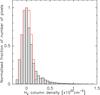 |
Fig. 5 Histogram of background-subtracted column density pixels (grey histogram) within a 10′ box centred on the central pixel displayed in Fig. 1. The column density noise estimated in each pixel (σj) corresponds to the dispersion of the red histogram, obtained by mirroring the negative part of the original histogram about its peak. |
SDC Herschel counterpart properties.
To decide whether an IRDC is real, we defined three criteria. The first one, c1, is the difference between the average Herschel column density within the τ8 μm boundary (as defined in Peretto & Fuller 2009, see Fig. 1) of the IRDC,  , and the average Herschel column density immediately outside this boundary,
  . By immediately outside we mean within the rectangular cutouts that have been defined in Peretto & Fuller (2009) to extract every SDC. The dimensions of these cutouts are twice the size of the SDC in both x and y directions (i.e. the image axes). If the IRDC is real, then we expect
  (3)The second parameter, c2, is defined as
  (4)where
  is the column density dispersion estimated on the scale of the cloud defined as
  (5)where npix is the number of pixels within the boundary of the IRDC, nbeam is the number of Herschel beams within the IRDC boundaries, θbeam = 18″ the resolution of the Herschel column density maps, and Req the equivalent angular radius of the IRDC (as defined in Peretto & Fuller 2009).
The third criterion, c3, is defined as  (6)This last criterion is more selective than c2, and as a result of eye investigation, we consider that a significant number of real IRDCs would be missed by using it, picking up very high signal-to-noise ratio clouds (an example of a SDC meeting c1 and c2 criteria but failing c3 is shown in Appendix A – SDC15.422-0.098). The detection results presented in this paper are based on c1 and c2 alone.
For each SDC, Table 1 gives the name, angular radius, , ,  , the peak H2 column density estimated with Herschel within the SDC boundary
  , c1 value, c2 value, c3 value, and the last column indicates whether the clouds satisfy the c1 and c2 criteria.
 |
Fig. 6 Number of SDCs (left) and automated detection fraction (right) as a function of SDC angular radius. |
The PF09 catalogue contains 8 SDCs that are not covered by Hi-GAL, and one that is located in a saturated portion of the 250 μm Herschel data, leaving a total of 11 287 SDCs for analysis. Figure 6 shows the histogram of SDC angular radius1, along with the histogram of the fraction of clouds satisfying criteria c1 and c2 per SDC size bin. For the remainder of this paper, we refer to this fraction as the automated detection fraction.
Using criteria c1 and c2, 63.2% (7,139) of the 11 287 SDCs of the PF09 catalogue are detected with Herschel. One can see in Fig. 6 that this detection fraction varies as a function of radius, with an increase up to an angular radius of 30′′, then a decrease down to Req ≃ 100′′, and a final increase at larger radius. This detection curve is affected by a number of elements that affect its interpretation. To get more insight into Fig. 6, we decided to simulate the SDC detection process.
 |
Fig. 7 Angular radius binned the same way as in Fig. 6 versus the median (red symbols and black solid line) peak extinction column densities of all SDCs from the PF09 catalogue. The purple solid lines and blue dashed lines are the 10/90 percentiles and 25/75 percentiles, respectively. |
4.2. Detection simulations
Because of the resolution difference between Herschel at 250 μm (18′′) and Spitzer at 8 μm (~2″), along with the strong fluctuations of the Galactic column density background, some of the smaller real SDCs may be missed by our identification scheme, while others might be wrongly classified as real. To evaluate the impact of background variations on our detection scheme, and therefore have a better estimate of the fraction of spurious clouds, we performed simulations of our cloud detection method.
Instead of taking idealised cloud models (Bonnor-Ebert spheres for instance), we decided to use SDCs themselves, since we believe they provide a more representative view of detection outcome. It is clear that large clouds with large column density peaks will be more easily detected than small and low-column density ones. To get a sample of SDCs that is representative of the full SDC population, we first computed the angular size versus peak column density (from extinction) for the SDCs from the PF09 catalogue. This is shown in Fig. 7. We can see that the peak column density is smoothly increasing up to Req ≃ 50″ and then increases rather sharply. The last two, and potentially even last three, points of this plot are heavily contaminated by spurious clouds though (cf below). Given this contamination, it seems likely that for real clouds, the trend observed below Req = 50″ continues to larger sizes. In any case, as we show below, all real clouds beyond an angular radius of 60′′ should be detected, no matter what, so for the modelling, we selected a sample of six SDCs whose sizes and column densities follow the median curve (black solid line) of Fig. 7, up to Req = 60″.
SDC visual inspection summary.
Using the PF09 Spitzer H2 column density maps, assuming a uniform temperature of either 12 K or 15 K (which is representative of the dust temperature of such clouds, Peretto et al. 2010) and the same dust opacity law and molecular weight as in Sect. 2, we inverted Eq. (2) to simulate the appearance of these six clouds at both 160 and 250 μm. We convolved these images to the Herschel resolutions and placed all six SDCs at 100 different locations within one of the nearly four square degree Hi-GAL tiles of the corresponding wavelength. The longitudes of each location were chosen to be regularly spaced, while the latitudes were randomly drawn from a normal distribution of FWHM = 1° and central position of −0.1°, as observed for our IRDC sample (see Fig. 11 of Peretto et al. 2009). We repeated the process for different Hi-GAL tiles between l = 10° and l = 63°. Finally, we applied our entire identification scheme (i.e. construction of colour column density images and detection criteria) for each modelled cloud. We also calculated c1 and c2 at the cloud location before adding them to the Herschel images (using the same τ8 μm = 0.35 boundaries as for our modelled SDCs – cf. Sect. 4). This allowed us to estimate the probability of having a positive detection even though no SDC is present and therefore gave us a sense of the contamination of the SDC automated detection fraction by spurious features.
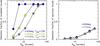 |
Fig. 8 Results of cloud detection simulations. Left: automated detection fraction of modelled SDCs as a function of SDC size for two different locations in the Galactic plane (i.e. l ~ 33° and l ~ 63°) and two different SDC dust temperature (i.e. 12 K and 15 K). Right: automated detection fraction of spurious clouds as a function of size for two different locations. |
Figure 8 displays the main results of our simulations. In the left-hand side panel, we can see that the fraction of modelled clouds that our automated detection scheme manages to identify strongly varies as a function of cloud sizes for all three longitudes displayed here. This fraction reaches 1 if the cloud is larger than 60′′ independently of the cloud temperature and location in the Galactic plane. For smaller clouds, the automated detection fraction depends on the cloud temperature and strength of the Galactic background (decreasing from the Galactic centre outwards). Modelled clouds with Req ≤ 10″ are the most difficult to identify with an automated detection fraction that could be as low as 0.1.
On the right-hand side panel of Fig. 8, one can see the fraction of spurious (i.e. non-existent) clouds that manage to pass criteria c1 and c2 and therefore would be considered as real according to our automated detection scheme. This fraction remains below 0.05 until the cloud reaches an angular radius of ~10″ and then smoothly increases up to ~0.3 for clouds with Req ≃ 100″. For the largest clouds of the PF09, the automated detection fraction of spurious clouds can reach 0.5 or more. These spurious detections are related to the probability of getting high column density peaks in a given area; i.e. the larger the area, the higher the probability. It also explains the break in the size column density plot of Fig. 7.
These simulations demonstrate that the automated detection fraction displayed in Fig. 6 is not easily interpreted. In the following section, we use the results of these simulations to further constrain the number of real SDCs in the PF09 catalogue.
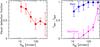 |
Fig. 9 Left: fraction of real SDCs as estimated through visual inspection (red symbols and solid line). Right: fraction of visually confirmed real SDCs that have been identified as real SDCs by our automated detection scheme (freal – blue round symbols), and fraction of visually confirmed spurious SDCs that have been misclassified as real SDCs by our automated detection scheme (fspur – purple square symbols). These two curves can directly be compared to our detection simulation results presented in Fig. 8. All error bars correspond to Poisson noise. |
5. Comparison between visual and automated detection fractions
5.1. Visual inspection
Visually inspecting a sub-sample of SDCs is an important step towards validating our detection scheme and simulations. We completed this step by visually matching the morphology of the SDCs as seen in the 8 μm Spitzer images with that of their Herschel column density counterparts. This can only be reliably done for rather large SDCs (i.e. at least the size of the Herschel beam). We thus focused on the six largest size bins of Fig. 6. We decided to check all 146 clouds falling in the last two bins of Fig. 6 (10 clouds in the last bin and 136 clouds in the one before), and 50 SDCs in each of the preceding four size bins. In practice, for each SDC we visually investigated, we overlaid the corresponding Herschel column density contours (starting from 0.1 × 1022 cm-2 and separated by steps of 0.5 × 1022 cm-2) on the Spitzer 8 μm image, and decided, after eye inspection, whether a column density peak was convincingly matching at least a portion of SDC. A sample of these images is provided in Appendix A. The detection fraction estimated this way is referred to as a visual detection fraction.
The left-hand side panel of Fig. 9 displays the visual detection fraction (column  of Table 2) as red symbols. We see that at large radii, the visual detection fraction is lower than the automated detection fraction as estimated for the same cloud sub-sample (column
  of Table 2). That the fraction of spurious clouds (column
  of Table 2) increases with size is a consequence of the construction of the 8 μm opacity maps that are built to identify the SDCs (Peretto & Fuller 2009). One step involves convolving the original Spitzer 8 μm images with a 5′ Gaussian kernel. This convolution is performed to construct the mid-infrared background image of the region. However, in places where a bright 8 μm region is present, this convolution artificially produces significant structures in the mid-infrared background, which translates into large spurious features in the 8 μm opacity maps (examples of such spurious clouds can be found in Appendix A, e.g. SDC329.368-0.437). On the other hand, at small radii, the visual detection fraction is greater. This is because the eye can more easily identify low signal-to-noise sources because it recognises matching shapes in Herschel and Spitzer images.
Assuming that the visual inspection provides the true fraction of real SDCs (the values in Table 2), we can compute the equivalent of Fig. 8 for the visually inspected sample of SDCs. For this, we first need to compute the fraction of SDCs in each size bin that have been misclassified as spurious sources by our automated detection scheme, nreal. We also need to evaluate the fraction of SDCs that have been misclassified as real sources by our automated detection scheme, nspur. With these numbers in hand, one can compute freal, the fraction of real SDCs that have been identified as real by our automated detection scheme. This is given by  , where is the fraction of visually confirmed SDCs (i.e. the visual detection fraction), and is the automated detection fraction for the same sub-sample of SDCs. This quantity is plotted as blue symbols in the right-hand side panel of Fig. 9, and is directly comparable to the left-hand side panel of Fig. 8. We can also compute fspur, the fraction of spurious SDCs that have been misclassified as real SDCs by our automated detection scheme. This is given by
  , where is the fraction of visually confirmed spurious SDCs. This quantity is plotted as purple symbols in the right-hand side panel of Fig. 9, and is directly comparable to the right-hand side panel of Fig. 8 (a summary of the visual inspection is given in Table 2). We can see that both trends (the increase in spurious detection fraction with increasing radius and the decrease in real SDC detection fraction with decreasing radius) were predicted by our detection simulations. The amplitude of these two effects are also reproduced well.
Overall, we can reasonably say that the large majority of SDCs with an angular radius under 60′′, which have been identified as real by our automated detection scheme, are indeed real. For larger clouds, visual inspection of individual sources is required to check their nature (real versus spurious). We note as well that the extinction-based column density and therefore sizes of the largest clouds appear comparatively uncertain. If any portion of one of these clouds was clearly associated with a Herschel column density peak, we then classified the clouds as real.
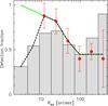 |
Fig. 10 Detection fraction as a function of SDC angular radius.The grey histogram is the same as in the right-hand side panel of Fig. 6. The red symbols are the same as in the left-hand side panel of Fig. 9. The black dashed and green solid lines represent the two assumptions that have been made for the fraction of real SDCs (Sect. 5.2). |
5.2. The fraction of real and spurious SDCs
The main unknown in determining the overall reliability of the SDCs is the detailed behaviour of the number of real clouds of small sizes that Herschel cannot resolve. For larger sources, a good estimate of the number of real SDCs as a function of size is provided by the visual detection fraction extrapolated to the entire sample. For the two smallest bins, the real SDC fraction remains unknown. However, given that the trend shows an increase in the number of real SDCs with decreasing sizes (as expected from the simulations), one could argue that the real SDC fraction must keep increasing for the two smallest size bins. The other extreme assumption one can make is that the real SDC fraction at these sizes is given by the automated detection fraction. These two hypotheses are represented in Fig. 10.
Taking the average of these two assumptions, one can now estimate the integrated real fraction of clouds over the entire sample. The percentage of real SDCs is estimated to be 76( ± 19)%; however for clouds with angular radius above 32′′, this percentage goes down to 55( ± 12)%. This decrease in the number of real clouds of large sizes is a reflection of the increased presence of artefacts in the 8 μm background images (see Sec. 5.1). The quoted uncertainties result from the combination of a 3% uncertainty related to the two different assumptions regarding the percentage of real small SDCs (see above); a 14% Poisson uncertainty per size bin related to the small number statistics of the visual inspection, going down to 6% when considering all six size bins and to 7% when only considering the four largest size bins; and finally a systematic error of 10% related to the visual real/spurious classification, which goes down to 5% when only considering the largest clouds (it is easier to visually characterise the nature of larger clouds).
It is worth noting that using SCUBA 850 μm data, Parsons et al. (2009) estimated that 75% of the 205 MSX IRDCs from the Simon et al. (2006) catalogue they analysed were real. This percentage is in total agreement with the detection fraction we provide here for the Spitzer IRDCs.
For comparison, we checked on a one-to-one basis our detection results with the one from Wilcock et al. (2012) for the l = [300°−330°] region. Where they identified 38% of the SDCs of this region as being Herschel bright, we detect 61%, which is only marginally less than the average over the entire sample. Of these 38% identified by Wilcock et al. (2012), 82% are also identified as real by our detection scheme. Of the remaining 18%, 72% have angular radius smaller than 16′′, corresponding to the size bins for which our identification scheme is less complete (see Fig. 10).
The clouds we positively identified but which were missed by Wilcock et al. (2012), i.e. 23% of the cloud population in the l = [300°−330°] region, are mostly low column density clouds that appear to be faint at 250 μm. This explains why they were missed, based on a visual inspection at that wavelength. An example of such a cloud is given in Fig. 1.
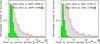 |
Fig. 11 Left: Herschel H2 peak column density histogram of Herschel-confirmed SDCs with a BGPS counterpart (grey histogram) and without a BGPS counterpart (green histogram). Right: same as the left-hand histogram but for ATLASGAL counterparts. The percentage of Herschel-confirmed SDCs in each category is indicated in the top right corner of each panel. |
6. Spitzer dark clouds in the BGPS and ATLASGAL
To characterise Spitzer dark clouds further, we cross-checked the Herschel-confirmed SDC sample against the catalogues of both BGPS (Rosolowsky et al. 2010) and ATLASGAL (Csengeri et al. 2014) (sub-)millimetre surveys. The differences in angular resolution, data type (emission versus extinction), and shapes of these sources make the association difficult to define. We considered that there was association between a SDC source and a BGPS/ATLASGAL source when the distance between the centroid positions of the two sources was less than the sum of their radii. The SDC radii are provided in Table 1 of this paper.
For the BGPS sources, we used the values quoted in Col. 10 of Table 1 of Rosolowsky et al. (2010). For ATLASGAL sources, we used, as source radius, the values quoted in Col. 8 of Table 1 of Csengeri et al. (2014). Figure 11 shows histograms of peak H2 column density (see Table 1) for Herschel-confirmed SDCs with and without BGPS counterparts (left panel) and real SDC with and without ATLASGAL counterparts (right panel). In this figure we can see that 1408 of the 2333 (60%) of the real SDCs covered by the BGPS have a BGPS counterparts while 925 (40%) do not. In this histogram it is clear that the latter represent the lowest column density (and smallest) SDCs of the catalogue. These are missed by BGPS as a result of their small sizes and their correspondingly small BGPS beam filling factor. In the right-hand panel of Fig. 11, one can see that only 1907 (27%) of the real SDCs covered by ATLASGAL have an ATLASGAL counterpart. This fraction is in good agreement with Contreras et al. (2013), who find an association fraction of 30%. Here again, SDCs without an ATLASGAL counterpart are mostly at low column density. The reason that the percentage of SDCs with BGPS sources is higher is the difference in the source identification schemes used in BGPS and ATLASGAL. The latter focused on the source identification on rather compact (upper limit of 50′′) and centrally concentrated (as imposed by the Gaussian fitting routine) sources. Such constraints are not imposed in the BGPS extraction. This comparison shows there is a rather large population of cold and compact sources that are missed by current (sub-)millimetre galactic plane surveys.
We also note that a large number of BGPS and ATLASGAL sources do not have SDC counterparts. While the majority of these sources are infrared bright sources, so cannot be associated, by definition, with an infrared dark cloud, some of them are infrared dark sources that have not been included in the the PF09 catalogue. Ellsworth-Bowers et al. (2013) identify a sub-sample of infrared dark BGPS sources and cross-checked against the SDCs from PF09. In their study, Ellsworth-Bowers et al. (2013) find that ~70% (based on their Fig. 15) of the sources from their sample are low-contrast infrared dark sources that remained undetected by PF09. In their paper, Ellsworth-Bowers et al. (2013) considered two sources to be associated if the distance between the centroid of the two sources is less than the semi-major axis of the SDC source. This is a very restrictive association condition for two main reasons. The first reason is linked to the definition of the semi-major axis. The semi-major axis σmaj of a SDC is defined as the column density weighed distance dispersion from the centroid position in the direction of the source major axis. Therefore, the disc of area  will have a much smaller area than
  where Req is the radius of the disc of the same area as the source, and BGPS sources outside the disc of radius σmaj will be missed.
The second reason is linked to the shape of SDCs. Sources with elongated or complicated shapes will have a large amount of their area beyond the association radius (even when considering the Req as the association radius), and very elongated filaments with BGPS sources at their tips, will be missed. This is exactly what happened for the source that Ellsworth-Bowers et al. (2013) use for illustration in their paper (BGPS # 5647) and for which they claim that the lower part of the cloud is not part of the PF09 catalogue, while it actually is (seen by looking at the image of SDC35.527-0.269 on www.irdarkclouds.org).
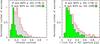 |
Fig. 12 Left: distribution of infrared contrast for BGPS sources associated with Herschel-confirmed SDCs (grey) and BGPS sources without SDC association (green). Right: same as in the left-hand panel but showing the distribution of BGPS 1.1 mm flux as estimated within a 40′′ aperture radius. The percentage of BGPS sources in each category is indicated in the top right corner of each panel. |
We therefore performed the association of IR dark BGPS sources with Herschel-confirmed SDC sources using the same association condition as previously and built the histograms of infrared contrast (see equation 11 of Ellsworth-Bowers et al. 2013) and BGPS 1.1 mm 40′′ aperture flux. Figure 12 displays these histograms. First, we see that, with our association condition, only 29% of BGPS sources are not associated to a SDC as opposed to 70% in Ellsworth-Bowers et al. (2013) analysis. In the left-hand panel of Fig. 12, we see that this population of sources mostly includes low infrared-contrast sources, as already noted by Ellsworth-Bowers et al. (2013). However, the corresponding distribution is much more peaked (see Fig. 15 of their paper). Looking at images of individual sources with contrast above 0.2, we also notice that these BGPS sources are, in fact, associated with SDCs. The reason for which we failed to associate these BGPS sources with SDCs is the same as the one mentioned above: an elongated BGPS source that includes a SDC at its tip can fail to pass the association criterion because the distance between the centroids of both sources can be larger that the sum of their Req radii. These same relatively high contrast sources are also the ones making the high-end tail of the 1.1 mm flux distribution in the right-hand panel of Fig. 12.
To determine the nature of the remaining low-contrast infrared dark BGPS sources without SDC association, we looked at both their BGPS and 8 μm Spitzer images. These sources appear to be mostly low column density IRDCs, as suggested by the position of the peak of 1.1 mm flux distribution with a large beam filling factor (as opposed to the population of low column density SDCs undetected in BGPS data – see green histogram in Fig. 11). These sources are either isolated sources or they lie in the low-density outskirts of denser clumps.
7. Summary and conclusion
Using Herschel Hi-GAL data, we constructed H2 column density images of the Galactic plane at 18′′ resolution using the 160 μm/250 μm ratio as a probe of the dust temperature. We used these data to determine the fraction of real IRDCs from the Peretto & Fuller (2009) catalogue by analysing their Herschel column density properties. Simulating the detection process, along with visually inspecting a small sub-sample of SDCs, shows that small angular size clouds are missed by our automated identification scheme as a result of beam dilution and large background fluctuations. On the other hand, very large features can be wrongly identified as real clouds owing to the probability of finding an Herschel column density peak in a given area of the Galactic plane. Taking these effects into account, we estimated that 76( ± 19)% of the SDCs are real. This fraction decreases to ~55( ± 12)% when considering clouds with an angular radius larger than ~30′′.
The availability of Herschel data towards the sources of the PF09 catalogue gives us the opportunity to analyse their far-infrared counterparts. As a result, the SDC properties are much better constrained, and studies of the earliest stages of Galactic star formation can now be more reliably performed on both individual and global scales. One particularly interesting feature of this Herschel-confirmed SDC sample is the broad range of cloud sizes and column densities it probes, providing a unique opportunity to study the link between the earliest stages of low- and high-mass star formation across the Milky Way.
The radii used here and quoted in Table 1 differ slightly from the ones in PF09. As a result of cloud reprojection a mistake had been made on the size of the pixel of the Spitzer images, which reflected in an over-estimate of the SDC radii up to 30%.
Acknowledgments
We thank the anonymous referee whose report helped improve the quality of this paper. N.P. acknowledges the support from the UK Science & Technology Facility Council (STFC) via grant ST/M000893/1. C.L. has been funded by a STFC Ph.D. studentship. G.A.F. and A.T. acknowledge the support from STFC via grant ST/J001562/1. M.A.T. acknowledges support from STFC via grant ST/M001008/1.
References
- Aguirre, J. E., Ginsburg, A. G., Dunham, M. K., et al. 2011, ApJS, 192, 4 [NASA ADS] [CrossRef] [MathSciNet] [Google Scholar]
- Battersby, C., Bally, J., Ginsburg, A., et al. 2011, A&A, 535, A128 [NASA ADS] [CrossRef] [EDP Sciences] [Google Scholar]
- Bernard, J.-P., Paradis, D., Marshall, D. J., et al. 2010, A&A, 518, L88 [NASA ADS] [CrossRef] [EDP Sciences] [Google Scholar]
- Churchwell, E., Babler, B. L., Meade, M. R., et al. 2009, PASP, 121, 213 [NASA ADS] [CrossRef] [Google Scholar]
- Contreras, Y., Schuller, F., Urquhart, J. S., et al. 2013, A&A, 549, A45 [NASA ADS] [CrossRef] [EDP Sciences] [Google Scholar]
- Csengeri, T., Urquhart, J. S., Schuller, F., et al. 2014, A&A, 565, A75 [NASA ADS] [CrossRef] [EDP Sciences] [Google Scholar]
- Ellsworth-Bowers, T. P., Glenn, J., Rosolowsky, E., et al. 2013, ApJ, 770, 39 [NASA ADS] [CrossRef] [Google Scholar]
- Griffin, M. J., Abergel, A., Abreu, A., et al. 2010, A&A, 518, L3 [Google Scholar]
- Hildebrand, R. H. 1983, Quant. J. Roy. Astron. Soc., 24, 267 [Google Scholar]
- Kauffmann, J., & Pillai, T. 2010, ApJ, 723, L7 [NASA ADS] [CrossRef] [Google Scholar]
- Molinari, S., Swinyard, B., Bally, J., et al. 2010, A&A, 518, L100 [NASA ADS] [CrossRef] [EDP Sciences] [Google Scholar]
- Molinari, S., Schisano, E., Elia, D., et al. 2016, A&A, in press, DOI: 10.1051/0004-6361/201526380 [Google Scholar]
- Ossenkopf, V., & Henning, T. 1994, A&A, 291, 943 [NASA ADS] [Google Scholar]
- Ott, S. 2010, in Astronomical Data Analysis Software and Systems XIX, eds. Y. Mizumoto, K.-I. Morita, & M. Ohishi, ASP Conf. Ser., 434, 139 [Google Scholar]
- Parsons, H., Thompson, M. A., & Chrysostomou, A. 2009, MNRAS, 399, 1506 [NASA ADS] [CrossRef] [Google Scholar]
- Perault, M., Omont, A., Simon, G., et al. 1996, A&A, 315, L165 [NASA ADS] [Google Scholar]
- Peretto, N., & Fuller, G. A. 2009, A&A, 505, 405 [NASA ADS] [CrossRef] [EDP Sciences] [Google Scholar]
- Peretto, N., & Fuller, G. A. 2010, ApJ, 723, 555 [NASA ADS] [CrossRef] [Google Scholar]
- Peretto, N., Fuller, G. A., Plume, R., et al. 2010, A&A, 518, L98 [NASA ADS] [CrossRef] [EDP Sciences] [Google Scholar]
- Peretto, N., Fuller, G. A., Duarte-Cabral, A., et al. 2013, A&A, 555, A112 [NASA ADS] [CrossRef] [EDP Sciences] [Google Scholar]
- Peretto, N., Fuller, G. A., André, P., et al. 2014, A&A, 561, A83 [NASA ADS] [CrossRef] [EDP Sciences] [Google Scholar]
- Piazzo, L., Calzoletti, L., Faustini, F., et al. 2015, MNRAS, 447, 1471 [NASA ADS] [CrossRef] [Google Scholar]
- Pilbratt, G. L., Riedinger, J. R., Passvogel, T., et al. 2010, A&A, 518, L1 [CrossRef] [EDP Sciences] [Google Scholar]
- Poglitsch, A., Waelkens, C., Geis, N., et al. 2010, A&A, 518, L2 [NASA ADS] [CrossRef] [EDP Sciences] [Google Scholar]
- Ragan, S. E., Bergin, E. A., & Gutermuth, R. A. 2009, ApJ, 698, 324 [NASA ADS] [CrossRef] [Google Scholar]
- Rathborne, J. M., Jackson, J. M., & Simon, R. 2006, ApJ, 641, 389 [NASA ADS] [CrossRef] [Google Scholar]
- Rosolowsky, E., Dunham, M. K., Ginsburg, A., et al. 2010, ApJS, 188, 123 [NASA ADS] [CrossRef] [Google Scholar]
- Schuller, F., Menten, K. M., Contreras, Y., et al. 2009, A&A, 504, 415 [NASA ADS] [CrossRef] [EDP Sciences] [Google Scholar]
- Simon, R., Jackson, J. M., Rathborne, J. M., & Chambers, E. T. 2006, ApJ, 639, 227 [NASA ADS] [CrossRef] [Google Scholar]
- Teyssier, D., Hennebelle, P., & Pérault, M. 2002, A&A, 382, 624 [NASA ADS] [CrossRef] [EDP Sciences] [Google Scholar]
- Traficante, A., Calzoletti, L., Veneziani, M., et al. 2011, MNRAS, 416, 2932 [NASA ADS] [CrossRef] [Google Scholar]
- Traficante, A., Fuller, G. A., Peretto, N., Pineda, J. E., & Molinari, S. 2015, MNRAS, 451, 3089 [NASA ADS] [CrossRef] [Google Scholar]
- Wilcock, L. A., Ward-Thompson, D., Kirk, J. M., et al. 2012, MNRAS, 424, 716 [NASA ADS] [CrossRef] [Google Scholar]
Appendix A: A sample of randomly selected SDCs
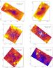 |
Fig. A.1 Images of 6 randomly selected SDCs. The colour scale is the Spitzer 8 μm emission. The black contour is the τ8 μm = 0.35 contour marking the boundary of the SDC as originally identified in PF09. The white contours are the Herschel H2 column density contours, all starting at 0.1 × 1022 cm-2, and separated by 0.5 × 1022 cm-2. The axes of the images are galactic coordinates in degrees. In the top right corner we give the name of the SDC and if our identification scheme has recognised them as being identified with a Herschel column density peak. SDC11.807-0.283 is not identified while, by eye, it seems clearly associated with a faint peak. Criterion c2 for this cloud is slightly below our threshold value of 3, explaining why it is not picked up by our identification scheme. |
 |
Fig. A.2 Same as Fig. A.1. The Herschel contours for SDC343.845-0.082 have been spaced by 1 × 1022 cm-2 (as opposed to 0.5 × 1022 cm-2 for the others) for clarity. |
All Tables
All Figures
|
Fig. 1 Images of SDC324.633+0.779. From left to right: Spitzer 8 μm image with the τ8 μm = 0.35 opacity contour showing the boundary of the SDC as defined in PF09; Herschel H2 column density map with background; Herschel background filtered H2 column density map; Herschel dust temperature map. |
| In the text | |
|
Fig. 2 Variation in R160/250, the ratio between 160 μm to 250 μm flux density as a function of dust temperature (see Eq. (1)). A value of 2 was adopted for the spectral index of the dust opacity law (i.e. β). |
| In the text | |
|
Fig. 3 Uncertainty linked to our column density construction method. In this plot we show the input IRDC column density versus the ratio of the retrieved column density versus true IRDC column density. The different colours correspond to different background properties. |
| In the text | |
|
Fig. 4 Ratio of the colour-based over SED column densities as a function of SED dust temperature for entire Hi-GAL tiles. The red solid line shows the average ratio over the corresponding tile, while the error bars represent one σ deviations. The blue dashed line indicates a ratio of 1. |
| In the text | |
|
Fig. 5 Histogram of background-subtracted column density pixels (grey histogram) within a 10′ box centred on the central pixel displayed in Fig. 1. The column density noise estimated in each pixel (σj) corresponds to the dispersion of the red histogram, obtained by mirroring the negative part of the original histogram about its peak. |
| In the text | |
|
Fig. 6 Number of SDCs (left) and automated detection fraction (right) as a function of SDC angular radius. |
| In the text | |
|
Fig. 7 Angular radius binned the same way as in Fig. 6 versus the median (red symbols and black solid line) peak extinction column densities of all SDCs from the PF09 catalogue. The purple solid lines and blue dashed lines are the 10/90 percentiles and 25/75 percentiles, respectively. |
| In the text | |
|
Fig. 8 Results of cloud detection simulations. Left: automated detection fraction of modelled SDCs as a function of SDC size for two different locations in the Galactic plane (i.e. l ~ 33° and l ~ 63°) and two different SDC dust temperature (i.e. 12 K and 15 K). Right: automated detection fraction of spurious clouds as a function of size for two different locations. |
| In the text | |
|
Fig. 9 Left: fraction of real SDCs as estimated through visual inspection (red symbols and solid line). Right: fraction of visually confirmed real SDCs that have been identified as real SDCs by our automated detection scheme (freal – blue round symbols), and fraction of visually confirmed spurious SDCs that have been misclassified as real SDCs by our automated detection scheme (fspur – purple square symbols). These two curves can directly be compared to our detection simulation results presented in Fig. 8. All error bars correspond to Poisson noise. |
| In the text | |
|
Fig. 10 Detection fraction as a function of SDC angular radius.The grey histogram is the same as in the right-hand side panel of Fig. 6. The red symbols are the same as in the left-hand side panel of Fig. 9. The black dashed and green solid lines represent the two assumptions that have been made for the fraction of real SDCs (Sect. 5.2). |
| In the text | |
|
Fig. 11 Left: Herschel H2 peak column density histogram of Herschel-confirmed SDCs with a BGPS counterpart (grey histogram) and without a BGPS counterpart (green histogram). Right: same as the left-hand histogram but for ATLASGAL counterparts. The percentage of Herschel-confirmed SDCs in each category is indicated in the top right corner of each panel. |
| In the text | |
|
Fig. 12 Left: distribution of infrared contrast for BGPS sources associated with Herschel-confirmed SDCs (grey) and BGPS sources without SDC association (green). Right: same as in the left-hand panel but showing the distribution of BGPS 1.1 mm flux as estimated within a 40′′ aperture radius. The percentage of BGPS sources in each category is indicated in the top right corner of each panel. |
| In the text | |
|
Fig. A.1 Images of 6 randomly selected SDCs. The colour scale is the Spitzer 8 μm emission. The black contour is the τ8 μm = 0.35 contour marking the boundary of the SDC as originally identified in PF09. The white contours are the Herschel H2 column density contours, all starting at 0.1 × 1022 cm-2, and separated by 0.5 × 1022 cm-2. The axes of the images are galactic coordinates in degrees. In the top right corner we give the name of the SDC and if our identification scheme has recognised them as being identified with a Herschel column density peak. SDC11.807-0.283 is not identified while, by eye, it seems clearly associated with a faint peak. Criterion c2 for this cloud is slightly below our threshold value of 3, explaining why it is not picked up by our identification scheme. |
| In the text | |
|
Fig. A.2 Same as Fig. A.1. The Herschel contours for SDC343.845-0.082 have been spaced by 1 × 1022 cm-2 (as opposed to 0.5 × 1022 cm-2 for the others) for clarity. |
| In the text | |
Current usage metrics show cumulative count of Article Views (full-text article views including HTML views, PDF and ePub downloads, according to the available data) and Abstracts Views on Vision4Press platform.
Data correspond to usage on the plateform after 2015. The current usage metrics is available 48-96 hours after online publication and is updated daily on week days.
Initial download of the metrics may take a while.