| Issue |
A&A
Volume 589, May 2016
|
|
|---|---|---|
| Article Number | A91 | |
| Number of page(s) | 13 | |
| Section | Interstellar and circumstellar matter | |
| DOI | https://doi.org/10.1051/0004-6361/201628229 | |
| Published online | 19 April 2016 | |
Clumpy dust clouds and extended atmosphere of the AGB star W Hydrae revealed with VLT/SPHERE-ZIMPOL and VLTI/AMBER⋆
1 Universidad Católica del Norte, Instituto de Astronomía, Avenida Angamos 0610, Antofagasta, Chile
e-mail: This email address is being protected from spambots. You need JavaScript enabled to view it.
2 Max-Planck-Institut für Radioastronomie, Auf dem Hügel 69, 53121 Bonn, Germany
Received: 31 January 2016
Accepted: 1 March 2016
Abstract
Context. Dust formation is thought to play an important role in the mass loss from stars at the asymptotic giant branch (AGB); however, where and how dust forms is still open to debate.
Aims. We present visible polarimetric imaging observations of the well-studied AGB star W Hya taken with VLT/SPHERE-ZIMPOL as well as high spectral resolution long-baseline interferometric observations taken with the AMBER instrument at the Very Large Telescope Interferometer (VLTI). Our goal is to spatially resolve the dust and molecule formation region within a few stellar radii.
Methods. We observed W Hya with VLT/SPHERE-ZIMPOL at three wavelengths in the continuum (645, 748, and 820 nm), in the Hα line at 656.3 nm, and in the TiO band at 717 nm. The VLTI/AMBER observations were carried out in the wavelength region of the CO first overtone lines near 2.3 μm with a spectral resolution of 12000.
Results. Taking advantage of the polarimetric imaging capability of SPHERE-ZIMPOL combined with the superb adaptive optics performance, we succeeded in spatially resolving three clumpy dust clouds located at ~50 mas (~2 R⋆) from the central star, revealing dust formation very close to the star. The AMBER data in the individual CO lines suggest a molecular outer atmosphere extending to ~3 R⋆. Furthermore, the SPHERE-ZIMPOL image taken over the Hα line shows emission with a radius of up to ~160 mas (~7 R⋆). We found that dust, molecular gas, and Hα-emitting hot gas coexist within 2–3 R⋆. Our modeling suggests that the observed polarized intensity maps can reasonably be explained by large (0.4–0.5 μm) grains of Al2O3, Mg2SiO4, or MgSiO3 in an optically thin shell (τ550nm = 0.1 ± 0.02) with an inner and outer boundary radius of 1.9–2.0 R⋆ and 3 ± 0.5R⋆, respectively. The observed clumpy structure can be reproduced by a density enhancement of a factor of 4 ± 1.
Conclusions. The grain size derived from our modeling of the SPHERE-ZIMPOL polarimetric images is consistent with the prediction of the hydrodynamical models for the mass loss driven by the scattering due to micron-sized grains. The detection of the clumpy dust clouds close to the star lends support to the dust formation induced by pulsation and large convective cells as predicted by the 3D simulations for AGB stars.
Key words: techniques: polarimetric / techniques: interferometric / stars: AGB and post-AGB / circumstellar matter / stars: individual: W Hya / stars: imaging
Based on SPHERE and AMBER observations made with the Very Large Telescope and Very Large Telescope Interferometer of the European Southern Observatory. Program ID: 095.D-0397(D) and 093.D-0468(A).
© ESO, 2016
1. Introduction
Low- and intermediate-mass stars experience significant mass loss at late stages of their evolution, particularly on the asymptotic giant branch (AGB). It is often argued that the levitation of the atmosphere by the large-amplitude stellar pulsation leads to dust formation, and the radiation pressure that the dust grains receive by absorbing stellar photons can initiate mass outflows. However, in the case of oxygen-rich AGB stars, the hydrodynamical simulations of Woitke (2006) and Höfner (2007) show that the radiation pressure on dust grains caused by the absorption of stellar photons is not sufficient to drive the mass loss with the mass-loss rates observed in these stars. The reason is that the iron-rich silicate, which efficiently absorbs stellar photons in the visible and near-IR and is therefore crucial for driving the mass loss, cannot exist in the vicinity of the star because the dust temperature exceeds the sublimation temperature. On the other hand, Al2O3 and the iron-poor silicate can exist much closer to the star because their opacity in the visible and near-IR is low. However, and exactly for this reason, it does not absorb stellar photons sufficiently to drive mass outflows. To solve this problem, Höfner (2008) proposes that the radiation pressure on micron-sized iron-free silicate grains due to scattering – and not to absorption – can drive outflows in oxygen-rich AGB stars.
High angular resolution observations have been revealing the presence of dust in the vicinity of the central star. The visible interferometric observations of Miras and semi-regular variables by Ireland et al. (2004) show an increase in the angular size toward shorter wavelengths, which is attributed to the increase in scattered light by dust in the inner circumstellar envelope. The long-baseline polarimetric interferometry of the Mira stars R Car and RR Sco carried out by Ireland et al. (2005) suggests the presence of transparent grains within 3 R⋆. More recently, Norris et al. (2012) have carried out polarimetric interferometry at 1.04–2.06 μm for three AGB stars (including W Hya presented in this paper) using the the aperture-masking technique with the NACO instrument of VLT. They measured the visibilities (i.e., amplitude of the Fourier transform of the intensity distribution of the object) in two perpendicular polarization directions. Because the visibility is sensitive to the size and shape of the object, the ratio of the visibilities measured in two polarization directions allowed them to detect scattered light from a dust shell very close to the star at 1.6–2 R⋆. Furthermore, they derived a grain size of ~0.3 μm, in agreement with the theory of Höfner (2008). Norris et al. (2012) suggest that iron-free silicates such as forsterite (Mg2SiO4) and enstatite (MgSiO3) or corundum (Al2O3) should be responsible for the scattering. The mid-IR interferometric observations of the semi-regular M giant RT Vir with the MIDI instrument at VLTI also lend support to the presence of iron-free silicate between 2 and 3 R⋆ (Sacuto et al. 2013).
The red giant W Hya is one of the well-studied oxygen-rich AGB stars. Thanks to its brightness and proximity ( pc, Knapp et al. 2003), it has been studied with various observational techniques from the visible to the radio. While it is classified as a semi-regular variable with spectral types of M7.5–9 on Simbad, its light curve shows clear periodicity (e.g., Woodruff et al. 2008) with a period of 389 days (Uttenthaler et al. 2011), although the variability amplitude of ΔV ≈ 3 is noticeably smaller than that of typical Mira stars. Therefore, it is often treated as a Mira star in the literature (see Uttenthaler et al. 2011 for a discussion of the classification).
Infrared interferometric observations of W Hya reveal an extended atmosphere. The uniform-disk diameter derived between 1.1 and 3.8 μm by Woodruff et al. (2008, 2009) shows that the angular size in the wavelength regions relatively free of H2O bands is 30–38 mas, while the angular size increases up to ~70 mas in the H2O bands, suggesting the presence of an H2O shell. The mid-IR interferometric observations of Zhao-Geisler et al. (2011) with VLTI/MIDI show that the angular diameter is 75–80 mas at 8–10 μm and increases to 100–105 mas from 10 to 13 μm. These authors interpret that the angular diameters at 8–10 μm represent the size of the H2O shell, while the increase in the angular diameter longward of 10 μm can be attributed to the dust envelope.
Khouri et al. (2015) present a detailed modeling of the dust envelope of W Hya using the spectral energy distribution (SED) and the dust spectral features observed from the near-IR to the sub-mm domain, as well as the aforementioned high spatial resolution observations of Norris et al. (2012) and Zhao-Geisler et al. (2011). The Khouri et al. model consists of a gravitationally bound shell of large (0.3 μm) grains of Al2O3 or Mg2SiO4 between 1.7 and 2.0 R⋆ and an outer amorphous silicate shell with an inner radius of >25 R⋆. They derived a current dust mass-loss rate of 4 × 10⁻¹⁰M⊙ yr-1 and suggest that there has been a change in the mass-loss rate of a factor of 2–3 within the last 4500 yr.
In this paper, we present visible polarimetric imaging observations of W Hya with the VLT/SPHERE-ZIMPOL instrument as well as high spatial and high spectral resolution near-IR interferometric observations with the VLTI/AMBER instrument. Our goal is to probe the dust and molecular gas close to the central star.
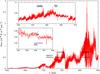 |
Fig. 1 High resolution visible spectrum of W Hya. The spectrum is based on the data obtained by Uttenthaler et al. (2011), and we applied the flux calibration to their spectrum as described in Sect. 2.1. The FWHMs of five filters used in our SPHERE-ZIMPOL observations are marked with the horizontal bars. The insets show enlarged views of the spectral region of the CntHa and NHa filters. The arrow in the lower inset marks the position of the Hα line. |
2. Observations
2.1. SPHERE-ZIMPOL polarimetric imaging observations
VLT/SPHERE is a high spatial resolution and high contrast imaging instrument mounted on the Unit Telescope (UT) 3; it is equipped with an extreme adaptive optics (AO) system for 0.55 to 2.32 μm (Beuzit et al. 2008). The ZIMPOL instrument is a module for nearly diffraction-limited polarimetric imaging (as well as classical, non-polarimetric imaging) at 550–900 nm (Thalmann et al. 2008). Our SPHERE-ZIMPOL observations of W Hya (Program ID: 095.D-0397, P.I.: K. Ohnaka) took place on 2015 July 08 (UTC) in P2 mode, in which the field orientation remained fixed. The K3III star HD 121653 (V = 7.2) was observed as a reference of the point spread function (PSF). The angular diameter of HD 121653 is 0.789 ± 0.022 mas (CalVin database1), which appears as a point source with the spatial resolution of SPHERE-ZIMPOL. The V magnitude of W Hya at the time of our SPHERE-ZIMPOL observations is estimated to be ~7, corresponding to phase 0.9 (pre-maximum light) of the light curve of the American Association of Variable Star Observers (AAVSO). The summary of our SPHERE-ZIMPOL observations is given in Table 1.
Summary of the SPHERE-ZIMPOL observations of W Hya.
We used five filters: CntHa (central wavelength λc = 644.9 nm, FWHM = 4.1 nm), NHa (λc = 656.34 nm, FWHM = 0.97 nm), TiO717 (λc = 716.8 nm, FWHM = 19.7 nm), Cnt748 (λc = 747.4 nm, FWHM = 20.6 nm), and Cnt820 (λc = 817.3 nm, FWHM = 19.8 nm). Figure 1 shows the high resolution spectrum of W Hya obtained by Uttenthaler et al. (2011) at nearly the same variability phase as our SPHERE-ZIMPOL observations (photometric calibration of the spectrum carried out as described below). The visible spectrum of W Hya is dominated by the prominent TiO bands. As the figure shows, three filters, CntHa, Cnt748, and Cnt820, sample the (pseudo-)continuum regions that are relatively free of TiO bands. The TiO717 filter samples the wavelength region of the TiO band. The NHa filter covers the wavelength region of the Hα line, as shown in the inset.
The SPHERE-ZIMPOL instrument, which is equipped with two cameras (cam1 and cam2), enables us to observe a given target with the same or different filters simultaneously. We observed W Hya by using the filter pairs of (CntHa, NHa), (TiO717, Cnt748), and (Cnt820, Cnt820) for cam1 and cam2. For the observations of W Hya with the Cnt820 filter, the neutral density filter ND1 was inserted in the path common to cam1 and cam2. The pixel scale of the two cameras is 3.628 mas. For each target and with each filter pair, we took Nexp exposures for each of the Stokes Q+, Q−, U+, and U− components, with NDIT frames in each exposure. We repeated this procedure at three different dithering positions.
The SPHERE instrument records the H-band Strehl ratios in separate FITS files2. As listed in Table 1, the median H-band Strehl ratio during the observations of W Hya was 0.79–0.88, which corresponds to Strehl ratios of 0.37–0.51 at the wavelengths of the ZIMPOL observations, if we assume that the Fried parameter is proportional to λ6/5. However, the median Strehl ratio during the observations of the PSF reference HD 121653 was significantly lower: 0.56–0.59 in the H-band. The Strehl ratios in the visible derived from the observed images of HD 121653 are 0.030–0.082 at the wavelengths of the ZIMPOL observations, which are 5–12 times lower than those for W Hya. The reason for the lower Strehl ratios for the PSF reference is likely the worse seeing during the observations of HD 121653 than for W Hya. Because of this significant difference in the AO performance between W Hya and the PSF reference, we did not deconvolve the images of W Hya.
We reduced the raw data using the SPHERE pipeline version 0.15.0-23. Each exposure was processed with the reduction pipeline, which produces the image of the Q+ or Q− or U+ or U− component as well as the intensity of each component (IQ+, IQ−, IU+, and IU−) for each camera. The output images were aligned and added to produce the average images of the polarization components and their associated intensity. Then the Stokes parameters I, Q, and U were computed as
 The polarized intensity IP and the degree of linear polarization pL as well as the position angle θ of the polarization vector were calculated from the Stokes parameters as follows:
  The orientation of the images was set so that north is up and east to the left, based on the following information kindly provided by M. van den Ancker in the User Support Department of ESO: the images on cam1 were up-down flipped, while those on cam2 were rotated by 180°. Since the position angle of the y-axis of the detector is 357.95°± 0.55°, the images (both cam1 and cam2) were rotated clockwise by 2.05°.
The flux of our PSF reference star HD 121653 with the filters used in our observations is not known, which means that we cannot use this star for the flux calibration of the SPHERE-ZIMPOL intensity maps of W Hya. Therefore, we carried out the flux calibration of the intensity maps using the high resolution visible spectrum of W Hya presented in Uttenthaler et al. (2011), which was obtained approximately at the same variability phase (although in a different variability cycle). We first scaled the spectrum so that the flux obtained with the V-band filter matches the V magnitude of 7 at the time of our SPHERE observations estimated from the AAVSO light curve. From this flux-calibrated visible spectrum of W Hya, we computed the flux for each filter used in our observations. We approximated the transmission curves of the filters with a top-hat function specified with the central wavelength and FWHM. The resulting fluxes with five filters are given in Table 2. The SPHERE-ZIMPOL intensity maps were scaled so that the flux integrated within a radius of 1.̋4 matches these fluxes. We chose this radius, because we needed to set the radius to be as large as possible to include the whole detected flux and still stay within the detector.
Flux derived for the five filters of our SPHERE-ZIMPOL observations of W Hya.
Summary of the VLTI/AMBER observations of W Hya and the calibrators.
2.2. High spectral resolution VLTI/AMBER observations
The near-IR VLTI instrument AMBER (Petrov et al. 2007), which operates at 1.3–2.4 μm, combines three UTs or 1.8 m Auxiliary Telescopes (ATs) and allows us to achieve a spatial resolution of 3 mas (at 2 μm) with the current maximum baseline of 140 m. The AMBER instrument is equipped with three spectral resolutions, 35, 1500, and 12 000. With the highest spectral resolution of 12 000, it is possible to resolve individual atomic and molecular lines. The interferometric observables measured with AMBER are visibility, closure phase (CP), and differential phase (DP). Visibility is the amplitude of the Fourier transform of the object’s intensity distribution on the sky and contains information about the size and shape of the object. The CP is the sum of the Fourier phases on three baselines around a triangle formed by three telescopes. Deviations of CP from 0 or 180° indicate asymmetry of the object. The DP represents the photocenter shift in spectral features with respect to the continuum. The AMBER instrument also records the spectrum of the same wavelength region simultaneously with the interferometric fringes.
We observed W Hya with VLTI/AMBER on 2014 April 22 (UTC) using the AT configuration A1-B2-C1, which covered projected baseline lengths from 7.0 to 13.3 m (Program ID: 093.D-0468, P.I.: K. Ohnaka). A summary of our AMBER observations is given in Table 3. The data taken at projected baselines shorter than 13.3 m correspond to the first visibility lobe of W Hya in the continuum (see Fig. 5c). Therefore, these data are appropriate for obtaining approximate sizes of the star and the extended atmosphere. The data with the projected baseline lengths shorter than the UT aperture of 8 m can be obtained with AO instruments, by speckle interferometry, or by aperture-masking and, if taken simultaneously, would be complementary to our AMBER data. However, with the absence of such single-dish data, the AMBER data points with projected baselines shorter than 8 m are important for constraining the size of the star. The variability phase at the time of our AMBER observations is estimated to be 0.77 from the AAVSO light curve (but in a different variability cycle). This is relatively close to the phase at the time of our SPHERE-ZIMPOL observations and allows us to measure the size of the dust shell in terms of the stellar radius. The wavelength region between 2.28 and 2.31 μm near the CO first overtone 2–0 band head was observed with the spectral resolution of 12 000. Thanks to the high brightness of W Hya (K ≈ −3, estimated from the K-band light curve of Whitelock et al. 2000), it was possible to achieve reasonable fringe S/N without the fringe tracker FINITO (W Hya saturates FINITO in the H-band). We observed α Cen A (G2V, K = −1.5, uniform-disk diameter = 8.314 ± 0.016 mas, Kervella et al. 2003) and Canopus (α Car, F0II) as an interferometric and spectroscopic calibrator, respectively.
The recorded fringes were processed with the amdlib version 3.0.84, which is based on the P2VM algorithm (Tatulli et al. 2007; Chelli et al. 2009). Details of the reduction are described in Ohnaka et al. (2009, 2011, and 2013). We checked for a systematic difference in the calibrated visibilities, CPs, and DPs by selecting the best 20% and 80% frames in terms of the fringe S/N. Since we did not detect any noticeable difference in the results, we took the best 80% of the frames, because the errors are smaller. The wavelength calibration and the spectroscopic calibration of the W Hya data were carried out with the method described in Ohnaka et al. (2009).
3. Results
3.1. SPHERE-ZIMPOL polarimetric images
3.1.1. Clumpy dust clouds
Figure 2 shows the intensity I, polarized intensity IP, and the degree of linear polarization pL of W Hya observed with five filters, together with the intensity of the PSF reference star HD 121653. The intensity maps of W Hya (first column of the figure) are noticeably more extended than the PSF reference images (fourth column of the figure), which means that the circumstellar envelope has been spatially resolved. This is clearly seen in the azimuthally averaged 1D intensity profiles of W Hya and HD 121653, which are plotted in Fig. 3a. The 2D Gaussian fit to the observed images of HD 121653 results in PSF FWHMs of 25 × 28 mas at 645 nm and 656.3 nm, 23 × 28 mas at 717 nm and 748 nm, and 24 × 30 mas at 820 nm.
The FWHM of the intensity distribution of W Hya at 645, 656.3, 717, and 820 nm is 53, 51, 58, and 46 mas, respectively. We note that the central region (within a radius of ≲20 mas) of the image at 748 nm is saturated, which makes is impossible to measure the FWHM (and also means that the flux calibration of the Cnt748 image is unreliable). Haniff et al. (1995) measured a Gaussian FWHM of 53.6 mas at 710 nm (filter FWHM = 10 nm). Ireland et al. (2004) measured the angular size of W Hya from 680 to 940 nm, and their FWHMs at the wavelengths of our observations are 75 mas (717 nm) and 42 mas (820 nm). The FWHM of our SPHERE-ZIMPOL image at 717 nm agrees with the result of Haniff et al. (1995), but is much smaller than that measured by Ireland et al. (2004). The FWHM measured at 820 nm by Ireland et al. (2004) agree with our value. We note that the observations of Ireland et al. (2004) were carried out at phase 0.44 (near minimum light), while our observations and the observations of Haniff et al. (1995) took place near maximum light, at phase 0.9 and 0.04, respectively. The angular size measurements of W Hya from 1.1 to 3.8 μm by Woodruff et al. (2009) show that the star appears smaller near maximum light than at minimum light. Therefore, the larger size measured by Ireland et al. (2004) than the present work or Haniff et al. (1995) may be due to the difference in the variability phase at the time of the observations.
While the intensity maps only show the global extended structure of the circumstellar envelope, the polarized intensity maps IP (second column in Fig. 2) reveal more detailed, clumpy structures of the innermost region of the envelope. We detected a large, bright clump in the north of the central star, another large clump in the SE, and a smaller clump in the SW. These clumps form an incomplete shell with a radius of ~50 mas. Moreover, as described in Sect. 3.2, the angular diameter of the central star measured in the continuum with AMBER is 46.6 mas. This means that the peak of the dust clumps is found at ~2 R⋆, and most of the clumps are located within ~3 R⋆ of the center of the star. In general, the polarized intensity represents the map of the optical depth, which is proportional to the column density of the scattering dust grains in an optically thin case (as presented in Sect. 4, this is the case for W Hya). Therefore, the obtained IP maps indeed reveal clumpy dust formation very close to the star, at ~2 R⋆. We note that since the saturation in the Cnt748 intensity map is limited to the central region with a radius of ~20 mas, it does not affect the clumpy features in the IP map with Cnt748. The radius of the dust formation region directly imaged in our SPHERE-ZIMPOL polarimetric imaging is consistent with the results of the polarimetric interferometric observations of Norris et al. (2012) and the modeling of 11.5 μm interferometric data of Wishnow et al. (2010).
Clumpy dust clouds are detected in other nearby AGB stars as well. For example, clumpy dust clouds have been imaged in the innermost circumstellar envelope of the well-studied carbon-rich AGB stars IRC+10216 (Weigelt et al. 1998; Haniff & Buscher 1998; Stewart et al. 2016 and references therein) and CIT6 (Monnier et al. 2000). Therefore, the formation of clumpy structures might be intrinsic to the mass loss phenomenon in AGB stars.
The errors in the polarized intensity (and in the degree of linear polarization as described below) were estimated using the output of the SPHERE pipeline. The relative errors in the polarized intensity are 3–5% at 645 nm, 4–8% at 656.3 nm, and ~2% at 717, 748, and 820 nm. In the region with very low polarized intensity near the center, which appears in dark blue between the clumps in the IP maps in Fig. 2, the relative errors amount to 50–60% at 645 and 656.3 nm, 40% at 717 nm, and 30% at 820 nm (since the central region of the IP map at 748 nm is affected by the aforementioned saturation issue, we excluded it from the error estimate of the central region).
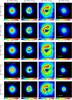 |
Fig. 2 Polarimetric imaging observations of W Hya with SPHERE-ZIMPOL. Each row shows the intensity (first column), polarized intensity (second column), degree of linear polarization with the polarization vector maps overlaid (third column), and the intensity of the PSF reference star HD 121653 (fourth column). The observed images at 645 nm (CntHa, continuum), 656.3 nm (NHa, Hα), 717 nm (TiO717, TiO band), 748 nm (Cnt748, continuum), and 820 nm (Cnt820, continuum) are shown from top to bottom. North is up and east to the left in all panels. The intensity maps and polarized intensity maps of W Hya, which are flux-calibrated as described in Sect. 2.1, are shown in units of W m-2μm-1 arcsec-2. The color scale of the intensity maps of W Hya and HD 121653 is cut off at 1% of the intensity peak. |
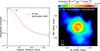 |
Fig. 3 a) Azimuthally averaged intensity profile of W Hya (red solid line) and the PSF reference HD 121653 (blue dashed line) obtained with the CntHa filter centered at 645 nm. b) Continuum-subtracted Hα image of W Hya derived from the SPHERE-ZIMPOL observations. |
The third column of Fig. 2 shows the maps of the degree of linear polarization at five wavelengths, with the polarization vector maps overlaid. The polarization vector maps, which show a concentric pattern, confirm the shell-like distribution of the clumps. The degree of linear polarization decreases slightly with wavelength: the maximum at 645, 656.3, 717, 748, and 820 nm is 13%, 12%, 10%, 9%, and 8%, respectively. The absolute errors in the degree of linear polarization in the clumps are 0.5% at 645 nm (i.e., pL = 13 ± 0.5%), 0.7% at 656.3 nm, 0.1% at 717 and 748 nm, and 0.2% at 820 nm. In the central region with very low degree of polarization, the absolute errors in pL are 0.1–0.2% at 645 and 656.3 nm, 0.03% at 717 nm, 0.04–0.07% at 820 nm.
The image of W Hya in the SO line at 215.2 GHz taken by Vlemmings et al. (2011) shows that the redshifted and blueshifted components are offset by 0.̋29 in the N-S direction, which the authors interpret as a bipolar outflow or a rotating disk. However, there is no signature of a bipolar outflow or a rotating disk in the SPHERE-ZIMPOL data probably because the dust formation close to the star is driven by large convective cells (see Sect. 5), which may mask the signatures of a bipolar structure or a rotating disk.
3.1.2. Extended Hα emission
The intensity map taken with the NHa filter including the Hα line (Fig. 2, first column, second row) appears to be more extended than the image taken with the CntHa filter sampling the nearby continuum (Fig. 2, first column, first row). In order to examine the presence of the Hα emission, we subtracted the CntHa image from the NHa image and both images were flux-calibrated as described in Sect. 2.1. Because the observations with the NHa and CntHa filters were carried out simultaneously, the performance of AO was the same for both filters. The continuum-subtracted Hα image shown in Fig. 3b reveals emission with a radius of ~100 mas (~4 R⋆); the emission in the south extends up to ~160 mas (~7 R⋆).
The extended Hα emission of W Hya is similar to the Hα envelope of the red supergiant Betelgeuse extending up to 5 R⋆ imaged by Hebden et al. (1987) and more recently by Kervella et al. (2016). While the extended Hα emission in Betelgeuse is thought to originate in the hot chromosphere, the Hα emission in Mira stars is associated with shocks induced by large amplitude stellar pulsation (e.g., Gillet et al. 1983a,b). Our Hα image of W Hya reveals the propagation of shocks as far as 4–7 R⋆. The presence of such extended Hα emission may not appear to be consistent with the weak Hα absorption seen in the visible spectrum shown in Fig. 1. However, this weak absorption can be interpreted as a result of the absorption being filled in by the extended emission.
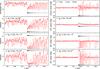 |
Fig. 4 VLTI/AMBER observations of W Hya with a spectral resolution of 12000 (data set #5). a) Observed spectrum. b)–d) Visibilities. e) Closure phase. f)–h) Differential phases. The positions of the CO lines are indicated by the ticks. |
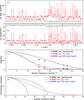 |
Fig. 5 Power-law-type limb-darkened disk fit to the AMBER data of W Hya. a) Limb-darkened disk diameter. The scaled observed spectrum of W Hya is shown by the black solid line. b) Limb-darkening parameter α. The black solid line represents the scaled observed spectrum with a vertical shift shown by the dashed line. c) Observed visibilities in the continuum, CO line, and CO band head are shown by the dots, while the visibilities from the limb-darkened disk fit are plotted by the solid lines. d) Limb-darkened disk intensity profiles in the continuum, CO line, and CO band head. |
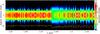 |
Fig. 6 Two-dimensional spectrum of W Hya computed from the limb-darkened disk fit shown in Fig. 5. The spatially unresolved spectrum is shown in yellow at the bottom. |
3.2. AMBER observations of the central star and molecular outer atmosphere
Figure 4 shows the visibilities, differential phases, and closure phase of W Hya observed with VLTI/AMBER from 2.28 to 2.31 μm (data set #5). In addition to the CO first overtone lines, a number of lines are present shortward of the CO band head at 2.2935 μm. They are mostly H2O and CN lines (e.g., Wallace & Hinkle 1996). To obtain an approximate angular size of the star as a function of wavelength, we fitted the observed visibilities with a power-law-type limb-darkened disk (Hestroffer et al. 1997) in which the intensity is described as I = [1−(p/R)2] α/ 2, where p, R, and α are the impact parameter, limb-darkened disk radius, and the limb-darkening parameter (α = 0 corresponds to a uniform disk).
Figure 5a shows the obtained limb-darkened disk diameter as a function of wavelength. On the one hand, the limb-darkened disk angular diameter is 46.6 ± 0.1 mas in the continuum and increases up to 230 mas in the CO lines. On the other hand, as Fig. 5b shows, the limb-darkening parameter α is modest in the continuum (2.1 ± 0.2; average and standard deviation over the continuum wavelengths), but much larger in the CO lines (20–40), suggesting significantly stronger limb-darkening in the CO lines. In Fig. 5d, we plot the limb-darkened disk intensity profiles at three representative wavelengths in the continuum, CO line, and CO band head. The limb-darkening is already remarkable in the continuum and so strong in the CO lines that it leads to Gaussian-like intensity profiles.
To better visualize the geometrical extension of the star in the continuum and in the lines, we generated a 2D spectrum as follows. First, the limb-darkened disk intensity profile at each wavelength is normalized so that the flux integrated over the stellar disk is equal to the observed flux at the corresponding wavelength. Then, the limb-darkened disk intensity profiles are color-coded and placed side by side. The resulting 2D spectrum (Fig. 6) reveals that the star shows a halo extending to a radius of ~70 mas (~3 R⋆) in the CO lines and to ~35 mas (~1.5 R⋆) in the weak H2O lines.
Figure 5c shows the fit to the visibilities at three wavelengths (continuum, CO bandhead, and CO line). The figure suggests that while the limb-darkened disk provides an approximate picture of the star’s intensity profile, there are noticeable deviations from the limb-darkened disk. The reduced χ2 values range from 2 to 100 with a median of 33.2 for the wavelengths covered by our observations. This means that the star is more complex than a symmetric limb-darkened disk, possibly with inhomogeneities. The detection of non-zero/non-180° DPs and CPs (see Figs. 4e–h) confirms the presence of such complex structures. This makes W Hya a good target for future aperture-synthesis imaging.
3.3. Coexistence of dust, CO gas, radio photosphere, SiO masers, and Hα-emitting hot gas
The extended atmosphere seen in the CO lines overlap with the location of clumpy dust clouds detected with SPHERE-ZIMPOL. Figure 7 shows the polarized intensity observed at 645 nm in color scale with the Hα emission represented in the contours. The geometrical extension of the atmosphere of ~70 mas (~3 R⋆), which is marked with the outer (yellow) circle in the figure, encompasses the extension of most of the dust clumps. The hot gas associated with the shocks traced with the Hα emission extends up to ~7 R⋆ and overlaps the distribution of the dust and CO gas.
Reid & Menten (2007) obtained an image of W Hya in the 43 GHz radio continuum with the Karl G. Jansky Very Large Array. The star shows extended emission – the so-called radio photosphere (Reid & Menten 1997) – that is 69 × 46 mas in size with the major axis lying nearly in the E–W direction. The size of the radio photosphere (blue ellipse in Fig. 7) is much smaller than the extension of the atmosphere seen in the 2.3 μm CO lines. The variability phase of the radio observations of Reid & Menten (2007) was 0.25, different from the phase of our AMBER observations. While this difference in the variability phase should be kept in mind, we also note that the temperature derived from the radio observations is rather high, 2380 ± 550 K. Therefore, the radio continuum at 43 GHz may sample the innermost region of the extended atmosphere. The SiO ν= 1, J = 1−0 masers imaged by Reid & Menten (2007) form an incomplete shell with a radius of 41 mas (middle black circle), coexisting with the CO gas and dust. These multi-wavelength observations suggest the complex, multicomponent nature of the outer atmosphere of W Hya.
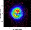 |
Fig. 7 Overlay of the distribution of dust (polarized intensity at 645 nm, color scale image), hot gas (Hα emission, contours), and the molecular gas (extension of the atmosphere derived from the AMBER data in the CO lines, outer yellow circle). The inner white circle represents the size of the star derived from the AMBER data in the continuum. The blue ellipse and the middle black circle represent the size of the radio photosphere and the SiO maser shell measured at 43 GHz by Reid & Menten (2007), respectively. The contours are plotted in logarithmic scale. The lowest and highest contours correspond to 3% and 100% of the maximum value, respectively. North is up, east to the left. |
4. Monte Carlo radiative transfer modeling of the polarized intensity maps
The SPHERE-ZIMPOL polarimetric images provide valuable constraints on the properties of the innermost dust envelope, particularly, the grain size. For this purpose, we used our Monte Carlo radiative transfer code mcmpi_sim (Ohnaka et al. 2006), which was also used for the interpretation of polarimetric imaging data (Murakawa et al. 2008). The change of the Stokes vector is treated with the scattering matrix (see, e.g., Wolf et al. 1999; Gordon et al. 2001), whose elements are computed from the complex refractive index of a given grain species. The output of our Monte Carlo code is the intensity (I) and the Stokes Q and U images. To compare these data with the observed values, we first convolved the model Q and U images, and also the intensity I with the observed PSF from the PSF reference star, and then computed the maps of the polarized intensity and the degree of linear polarization from the convolved Q, U, and I images. We adopted this approach instead of convolving the model IP and pL maps because it corresponds to how the IP and pL maps were obtained from the observational data.
However, as Fig. 3a shows, the 1D intensity profile of our PSF reference star HD 121653 shows a halo that is more extended than that of W Hya at intensity levels lower than 1% of the central peak (at angular distances greater than 120 mas), although HD 121653 should appear as a point source. This means that the performance of AO was much worse for HD 121653 than for W Hya due to the worse seeing (see in Sect. 2.1). If we convolve the model I images with the PSF from HD 121653, this extended halo in the PSF – despite its low intensity – makes the convolved I images much more extended than it should be with the true, narrower PSF for W Hya. When the convolved I images are too extended, the predicted degree of polarization is significantly lower because of the division with I in pL = IP/I, which makes a comparison with the observed data impossible. However, we found out that the polarized intensity maps normalized with the peak value at each wavelength are not very sensitive to the extended halo of the observed PSF. Therefore, we used the normalized polarized intensity maps to constrain the properties of the inner dust envelope.
In our modeling, we computed the polarized intensity maps at the wavelengths observed with SPHERE-ZIMPOL and also the fraction of scattered light in the near-IR wavelengths studied by Norris et al. (2012). While our visible polarimetric imaging data allow us to constrain the properties of the innermost circumstellar environment, they cannot constrain the properties of grain species that give rise to the IR features. Therefore, we did not attempt to fit the SED. As mentioned in Sect. 1, Khouri et al. (2015) carried out a detailed modeling of the SED, including various dust features.
The radiation of the central star was approximated with a blackbody of 2500 K as in Khouri et al. (2015). We adopted an angular diameter of 46.6 mas measured in the continuum with AMBER, which results in a radius of 383 R⊙ and a luminosity of 5130 L⊙ when combined with the distance of 78 pc from Knapp et al. (2003).
To explain the clumpy structure seen in the polarized intensity maps, we considered a dust shell model with a density enhancement, which is defined by a cone as depicted in Fig. 8a. The inner boundary of the dust shell was set to be the radius at which the dust temperature reaches a condensation temperature of 1500 K. We assumed the radial density distribution to be ∝r-3 for the following reason. While the density distribution proportional to r-2 corresponds to a stationary mass loss with a constant velocity, the density gradient in the innermost region of the envelope is expected to be steeper because the wind speed should increase at the base of the stellar wind. This is supported by the mid-infrared interferometric observations of Mira stars by Karovicova et al. (2013). These data probe the inner region of the circumstellar envelope, and their modeling shows that the power-law index of the density distribution of Al2O3 is 2.5–2.9.
The free parameters in our clump model are the optical depth in the visible (550 nm) in the radial direction, the outer boundary radius of the shell, the half-opening angle of the cone of the density enhancement, and the ratio of the density in the cone and in the remaining region of the shell. We considered three grain species, corundum (Al2O3), forsterite (Mg2SiO4), and enstatite (MgSiO3), because they are thought to survive at high temperatures thanks to their low opacity in the visible and near-IR. The absorption and scattering cross sections, as well as the scattering matrix elements, were computed with the code of Bohren & Huffman (1983) for spherical grains, using the complex refractive index measured by Koike et al. (1995) for Al2O3 and the measurements of Jäger et al. (2003) for Mg2SiO4 and MgSiO3. We also computed models with the complex refractive index of Mg2SiO4 and MgSiO3 measured by Scott & Duley (1996) to examine possible effects of different measurements.
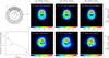 |
Fig. 8 Dust clump model of W Hya. a) Schematic view of our model. The hatched region is the spherical dust shell. The cross-hatched region represents a cone-shaped density enhancement, which is characterized by the half-opening angle θ. The viewing angle of the model is also shown. b) Fraction of scattered light derived by Norris et al. (2012) is plotted by the red dots (the errors are approximately the same as the size of the dots), while the model prediction is shown by the blue solid line. c)–h) Model and observed polarized intensity maps at 645, 717, and 820 nm. North is up, east to the left. |
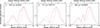 |
Fig. 9 North-south 1D cuts of the polarized intensity of W Hya at 645 nm (panel a)), 717 nm (panel b)), and 820 nm (panel c)). In each panel, the red solid line represents the observed data, while the blue dashed line represents the model. |
Figure 8 shows the IP maps at 645, 717, and 820 nm predicted by the best-fit model with 0.5 μm Al2O3 grains together with the observed data. This model is characterized by a density enhancement with a half-opening angle of 45° and a density ratio of 4 within and outside the cone. The inner and outer boundary radius is 1.9 and 3 R⋆, respectively, and the 550 nm optical depth is 0.1. As Fig. 8a shows, the viewing angle measured from the symmetry axis is 85°. The density enhancement manifests itself as asymmetry in the IP maps. The ratio of the polarized intensity measured on the brightest clump in the north and the faintest clump in the SW in the SPHERE-ZIMPOL data is 2.7, 2.5, and 1.8 at 645 nm, 717 nm, and 820 nm, respectively. The model predicts the ratio to be 2.3, 2.1, and 2.4 at 645, 717, and 820 nm, respectively, which agree with the observed ratios. Figure 9 shows the 1D cuts of the observed and model polarized intensity in the north-south direction. The figure shows that our model can reproduce the observed ratio of the polarized intensity peaks reasonably well given the simplifications adopted in the model. However, the polarized intensity at the center of this model is much lower than the observed data. We assumed a density enhancement in only one direction, while we detected three clumps possibly with different density enhancements. Therefore, density distributions that are more complex than assumed here may reconcile the discrepancy in the polarized intensity near the center.
Figure 8b shows a comparison of the predicted fraction of scattered light at 1.04, 1.24, and 2.06 μm and the observed values from Norris et al. (2012). The fraction of scattered light predicted by the model agrees fairly well with the observed values, although the model predicts that the fraction should be higher than the observed value by a factor of ~2 at 2.06 μm. However, Norris et al. (2012) assumed a geometrically thin spherical shell to derive the fraction of scattered light. Furthermore, the variability phase at the time of their observations was 0.2 (post-maximum light), in contrast to the phase 0.9 of our SPHERE observations. These factors may explain the discrepancy of a factor of 2 at 2.06 μm.
The parameters derived from our models with Mg2SiO4 or MgSiO3 are similar to those of the best-fit model with Al2O3. The results obtained with the complex refractive indices of Mg2SiO4 and MgSiO3 measured by Scott & Duley (1996) also agree with those obtained with the data of Jäger et al. (2003). Our modeling with three grain species results in a 550 nm optical depth of 0.1 ± 0.02 with grain sizes of 0.4–0.5 μm, and an inner and outer boundary radius of 1.9–2.0 R⋆ (defined by the assumed condensation temperature of 1500 K) and 3 ± 0.5R⋆. The density enhancement is characterized by a half-opening angle of 45°±15° and a density ratio of 4 ± 1. For the half-opening angle of 45°, viewing angles between 60° and 100° (measured from the symmetry axis as shown in Fig. 8a) reproduce the observed ratios of the polarized intensity between the brightest and faintest clumps. As we explain in the next section, the models with a grain size smaller than ~0.3 μm cannot reproduce the observed polarized intensity maps. On the other hand, if the grain size is larger than ~0.6 μm, the predicted fractions of scattered light at 1.04, 1.24, and 2.06 μm are much higher than the observed values from Norris et al. (2012).
5. Discussion
The grain size of 0.4–0.5 μm derived from our modeling is larger than the 0.3 μm derived by Norris et al. (2012). If the grain radius of 0.3 μm is adopted in our model, the 550 nm optical depth should be increased to 0.5 to explain the observed fraction of scattered light from 1.04 to 2.06 μm. Then the optical depth along the line of sight grazing the inner boundary of the dust shell becomes much larger than 1, even if the optical depth in the radial direction is still below 1. Multiple scattering for an optical depth larger than 1 leads to very low polarization at the inner boundary, which is not observed in our SPHERE-ZIMPOL data. However, given the differences in the observational data, variability phase, and the assumptions in the models, the difference between the 0.3 μm derived by Norris et al. (2012) and the 0.4–0.5 μm from our modeling does not seem to be serious. The dust mass from our model is 5.8 × 10⁻¹⁰M⊙ with a bulk density of 4 g cm-3 adopted for Al2O3. This is comparable to the (1.09 ± 0.02) × 10-9M⊙ estimated by Norris et al. (2012), despite the difference in the grain size. The dust mass from our model also agrees well with 4.9 × 10⁻¹⁰M⊙ derived by Khouri et al. (2015), who also assumed a grain size of 0.3 μm. Therefore, our modeling based on the SPHERE-ZIMPOL polarimetric images confirms the predominance of large, transparent grains in W Hya very close to the star, ~2 R⋆, and reveals that the grain size is even larger than derived by Norris et al. (2012).
Höfner (2008) presents dynamical models with the mass loss driven by the scattering of stellar photons. The parameters of these models (stellar mass, luminosity, effective temperature, and pulsation period) are comparable to those of W Hya, if not perfectly optimized for W Hya. The models predict that the grain size can reach 0.36–0.66 μm at 2–3 R⋆. The grain size of 0.4–0.5 μm as well as the inner radius of the dust shell derived from our modeling agrees with these predictions, lending support to the scenario that the scattering due to large, transparent grains can drive the mass loss in oxygen-rich AGB stars.
In the dynamical models of Höfner (2008), however, the nucleation of dust grains from the gas phase is not considered. While the growth of Mg2SiO4 grains is followed in a time-dependent manner, the presence of seed nuclei is assumed, and their amount is treated as a free parameter. Gobrecht et al. (2016, and references therein) present comprehensive models for non-equilibrium chemical processes of gas and dust in the inner wind of AGB stars, incorporating the nucleation of dust grains from the gas phase, although dynamical aspects such as the radiation pressure on dust grains and the mass loss are not included. Their models predict that Al2O3 forms within 2 R⋆, and that the grain radius reaches 0.3 μm in some cases. These model predictions are consistent with our results, given that the models of Gobrecht et al. (2016) are optimized for the Mira star IK Tau, which is more evolved than W Hya. Their models predict that Mg2SiO4 forms beyond 3 R⋆ and that MgSiO3 is far less abundant than Mg2SiO4. Therefore, Al2O3, rather than iron-poor silicates, may be the more plausible constituent of the clumpy dust clouds detected in our SPHERE-ZIMPOL observations. Adjusting these models for W Hya would allow us to test the non-equilibrium chemistry using the present data.
The observed polarized intensity maps suggest that a few large dust clumps nearly cover the entire sphere. In the case of the model shown in Fig. 8, the solid angle of the density enhancement is 4π × 0.15 str, which means that approximately seven clumps can cover the entire sphere. Freytag & Höfner (2008) present 3D convective simulations for AGB stars with dust formation. Their models show that the stellar surface is covered by a few, large convective cells and that the star pulsates with a typical time scale of one year. Dust forms behind the shock fronts associated with the pulsation and the convective cells. The dust formation region appears nearly spherical but with noticeable irregularities of the size of the convective cells. Although their 3D models assume a carbon-rich chemistry unlike that of W Hya, a similar phenomenon may be expected in oxygen-rich cases as well. The polarized intensity maps obtained with SPHERE-ZIMPOL show similar signatures – dust formation in an incomplete shell with clumpy structures. Therefore, our SPHERE-ZIMPOL observations lend support to the dust formation associated with the shocks induced by the pulsation and convection.
6. Concluding remarks
We have presented visible polarimetric imaging observations of the AGB star W Hya with SPHERE-ZIMPOL and high spectral resolution (λ/ Δλ = 12 000) interferometric observations with VLTI/AMBER in the individual CO first overtone lines near 2.3 μm. The polarized intensity maps obtained at five wavelengths between 645 and 820 nm with spatial resolutions of 23–30 mas reveal three clumpy dust clouds close to the star, at ~50 mas (~2 R⋆). The continuum-subtracted Hα image shows asymmetrically extended emission up to ~160 mas, implying the propagation of shocks up to ~7 R⋆.
The VLTI/AMBER observations have allowed us to spatially resolve the outer atmosphere of W Hya. The fitting of the AMBER data in the continuum in the 2.3 μm region with a power-law-type limb-darkened disk resulted in a stellar diameter of 46.6 ± 1.0 mas with a limb-darkening parameter of 2.1 ± 0.2. On the other hand, the AMBER data in the CO lines suggest that the atmosphere is extended to ~70 mas (~3 R⋆) with Gaussian-like intensity distributions. Our high angular resolution observations with SPHERE-ZIMPOL and VLTI/AMBER reveals the coexistence of dust, molecular gas, and Hα-emitting hot gas within 2–3 R⋆.
Our Monte Carlo radiative transfer modeling suggests the presence of 0.4–0.5 μm grains of Al2O3, Mg2SiO4, or MgSiO3 in an optically thin (τ550 nm = 0.1 ± 0.02) shell with an inner and outer radius of 1.9–2 R⋆ and 3 ± 0.5R⋆, respectively. The grain size and the location of the dust formation is consistent with the hydrodynamical models with the mass loss driven by the scattering due to large grains. The clumpy structures detected in the SPHERE-ZIMPOL polarimetric images lend support to the 3D simulations, in which dust forms behind the shock fronts associated with pulsation and large convective cells.
Our SPHERE-ZIMPOL observations took place at pre-maximum light. Given the clear periodicity in the light curve of W Hya, monitoring observations with SPHERE-ZIMPOL following the variability phase is extremely important in order to understand the role of pulsation in dust formation and mass loss. Moreover, the velocity-resolved imaging with VLTI/AMBER taking advantage of its high spatial and high spectral resolution enables us to probe the gas dynamics in a model-independent manner. The velocity-resolved imaging in the CO lines and H2O lines is ideal for detecting the initial acceleration of gas within ~3 R⋆ and, therefore, is indispensable for clarifying the driving mechanism of the mass loss.
Classified as “OBJECT, AO” in the ESO data archive.
Available at ftp://ftp.eso.org/pub/dfs/pipelines/sphere
Available at http://www.jmmc.fr/data_processing_amber.htm
Acknowledgments
We thank the ESO Paranal team for supporting our SPHERE and AMBER observations and Henning Avenhaus for helping us optimize the instrumental set-up of our SPHERE observations. We are also grateful to Mario van den Ancker and Julien Girard for providing us with the information about the orientation of the SPHERE-ZIMPOL detectors and the information about the data files with parameters relevant to the AO performance including the Strehl ratios. This research made use of the SIMBAD database, operated at the CDS, Strasbourg, France. We acknowledge with thanks the variable star observations from the AAVSO International Database contributed by observers worldwide and used in this research.
References
- Beuzit, J.-L., Feldt, M., Dohlen, K., et al. 2008, SPIE Proc., 7014, 18 [NASA ADS] [Google Scholar]
- Bohren, C. F., & Huffman, D. R. 1983, Absorption and Scattering of Light by Small Particles (New York: Wiley) [Google Scholar]
- Chelli, A., Hernandez Utrera, O., & Duvert, G. 2009, A&A, 502, 705 [NASA ADS] [CrossRef] [EDP Sciences] [Google Scholar]
- Freytag, B., & Höfner, S. 2008, A&A, 483, 571 [NASA ADS] [CrossRef] [EDP Sciences] [Google Scholar]
- Gillet, D., Maurice, E., & Baade, D. 1983a, A&A, 128, 384 [NASA ADS] [Google Scholar]
- Gillet, D., Ferlet, R., Maurice, E., & Bouchet, P. 1983b, A&A, 128, 384 [NASA ADS] [Google Scholar]
- Gobrecht, D., Cherchneff, I., Sarangi, A., Plane, J. M. C., & Bromley, S. T. 2016, A&A, 585, A6 [NASA ADS] [CrossRef] [EDP Sciences] [Google Scholar]
- Gordon, K., Misselt, K. A., Witt, A. N., & Clayton, G. C. 2001, ApJ, 551, 269 [NASA ADS] [CrossRef] [Google Scholar]
- Haniff, C. A., & Buscher, D. F. 1998, A&A, 334, L5 [NASA ADS] [Google Scholar]
- Haniff, C. A., Scholz, M., & Tuthill, P. G. 1995, MNRAS, 276, 640 [NASA ADS] [CrossRef] [Google Scholar]
- Hebden, J. C., Eckart, A., & Hege, E. K. 1987, ApJ, 314, 690 [NASA ADS] [CrossRef] [Google Scholar]
- Hestroffer, D. 1997, A&A, 327, 199 [NASA ADS] [Google Scholar]
- Höfner, S. 2007, ASP Conf. Ser., 378, 145 [NASA ADS] [Google Scholar]
- Höfner, S. 2008, A&A, 491, L1 [NASA ADS] [CrossRef] [EDP Sciences] [Google Scholar]
- Ireland, M. J., Tuthill, P. G., Bedding, T. R., Robertson, J. G., & Jacob, A. P. 2004, MNRAS, 350, 365 [NASA ADS] [CrossRef] [Google Scholar]
- Ireland, M. J., Tuthill, P. G., Davis, J., & Tango, W. 2005, MNRAS, 361, 337 [NASA ADS] [CrossRef] [Google Scholar]
- Jäger, C., Dorschner, J., Mutschke, H., Posch, T., & Henning, Th. 2003, A&A, 408, 193 [NASA ADS] [CrossRef] [EDP Sciences] [Google Scholar]
- Karovicova, I., Wittkowski, M., Ohnaka, K., et al. 2013, A&A, 560, A75 [NASA ADS] [CrossRef] [EDP Sciences] [Google Scholar]
- Kervella, P., Thévenin, F., Ségransan, D., et al. 2003, A&A, 404, 1087 [NASA ADS] [CrossRef] [EDP Sciences] [Google Scholar]
- Kervella, P., Lagadec, E., Montargès, M., et al. 2016, A&A, 585, A28 [NASA ADS] [CrossRef] [EDP Sciences] [Google Scholar]
- Khouri, T., Waters, L. B. F. M., de Koter, A., et al. 2015, A&A, 577, A114 [NASA ADS] [CrossRef] [EDP Sciences] [Google Scholar]
- Knapp, G. R., Pourbaix, D., Platais, I., & Jorissen, A. 2003, A&A, 403, 993 [NASA ADS] [CrossRef] [EDP Sciences] [Google Scholar]
- Koike, C., Kaito, C., Yamamoto, T., et al. 1995, Icarus, 114, 203 [NASA ADS] [CrossRef] [Google Scholar]
- Monnier, J. D., Tuthill, P. G., & Danchi, W. C. 2000, ApJ, 545, 957 [NASA ADS] [CrossRef] [Google Scholar]
- Murakawa, K., Ohnaka, K., Driebe, T., et al. 2008, A&A, 489, 195 [NASA ADS] [CrossRef] [EDP Sciences] [Google Scholar]
- Norris, B., Tuthill, P. G., Ireland, M. J., et al. 2012, Nature, 484, 220 [NASA ADS] [CrossRef] [PubMed] [Google Scholar]
- Ohnaka, K., Driebe, T., Hofmann, K.-H., et al. 2006, A&A, 445, 1015 [NASA ADS] [CrossRef] [EDP Sciences] [Google Scholar]
- Ohnaka, K., Hofmann, K.-H., Benisty, M., et al. 2009, A&A, 503, 183 [NASA ADS] [CrossRef] [EDP Sciences] [Google Scholar]
- Ohnaka, K., Weigelt, G., Millour, F., et al. 2011, A&A, 529, A163 [NASA ADS] [CrossRef] [EDP Sciences] [Google Scholar]
- Ohnaka, K., Hofmann, K-.H., Schertl, D., et al. 2013, A&A, 555, A24 [NASA ADS] [CrossRef] [EDP Sciences] [Google Scholar]
- Petrov, R. G., Malbet, F., Weigelt, G., et al. 2007, A&A, 464, 1 [NASA ADS] [CrossRef] [EDP Sciences] [Google Scholar]
- Reid, M. J., & Menten, K. M. 1997, ApJ, 476, 327 [NASA ADS] [CrossRef] [Google Scholar]
- Reid, M. J., & Menten, K. M. 2007, ApJ, 671, 2068 [NASA ADS] [CrossRef] [Google Scholar]
- Sacuto, S., Ramstedt, S., Höfner, S., et al. 2013, A&A, 551, A72 [NASA ADS] [CrossRef] [EDP Sciences] [Google Scholar]
- Scott, A., & Duley, W. W. 1996, ApJS, 105, 401 [NASA ADS] [CrossRef] [Google Scholar]
- Stewart, P. N., Tuthill, P. G., Monnier, J. D., et al. 2016, MNRAS, 455, 3102 [NASA ADS] [CrossRef] [Google Scholar]
- Tatulli, E., Millour, F., Chelli, A., et al. 2007, A&A, 464, 29 [NASA ADS] [CrossRef] [EDP Sciences] [Google Scholar]
- Thalmann, C., Schmid, H. M., Boccaletti, A., et al. 2008, SPIE Proc., 70143 [Google Scholar]
- Uttenthaler, S., Van Stiphout, K., Voet, K., et al. 2011, A&A, 531, A88 [NASA ADS] [CrossRef] [EDP Sciences] [Google Scholar]
- Vlemmings, W. H. T., Humphreys, E. M. L., & Franco-Hernández, R. 2011, ApJ, 728, 149 [NASA ADS] [CrossRef] [Google Scholar]
- Wallace, L., & Hinkle, K. H. 1996, ApJS, 107, 312 [NASA ADS] [CrossRef] [Google Scholar]
- Weigelt, G., Balega, Y., Blöcker, T., et al. 1998, A&A, 333, L51 [NASA ADS] [Google Scholar]
- Whitelock, P., Marang, F., & Feast, M. 2000, MNRAS, 319, 728 [NASA ADS] [CrossRef] [Google Scholar]
- Wishnow, E. H., Townes, C. H., Walp, B., & Lockwood, S. 2010, ApJ, 712, L135 [NASA ADS] [CrossRef] [Google Scholar]
- Woitke, P. 2006, A&A, 460, L9 [NASA ADS] [CrossRef] [EDP Sciences] [Google Scholar]
- Wolf, S., Henning, Th., & Stecklum, B. 1999, A&A, 349, 839 [Google Scholar]
- Woodruff, H. C., Tuthill, P. G., Monnier, J. D., et al. 2008, ApJ, 673, 418 [NASA ADS] [CrossRef] [Google Scholar]
- Woodruff, H. C., Ireland, M. J., Tuthill, P. G., et al. 2009, ApJ, 691, 1328 [NASA ADS] [CrossRef] [Google Scholar]
- Zhao-Geisler, R., Quirrenbach, A., Köhler, R., Lopez, B., & Leinert, C. 2011, A&A, 530, A120 [NASA ADS] [CrossRef] [EDP Sciences] [Google Scholar]
All Tables
All Figures
|
Fig. 1 High resolution visible spectrum of W Hya. The spectrum is based on the data obtained by Uttenthaler et al. (2011), and we applied the flux calibration to their spectrum as described in Sect. 2.1. The FWHMs of five filters used in our SPHERE-ZIMPOL observations are marked with the horizontal bars. The insets show enlarged views of the spectral region of the CntHa and NHa filters. The arrow in the lower inset marks the position of the Hα line. |
| In the text | |
|
Fig. 2 Polarimetric imaging observations of W Hya with SPHERE-ZIMPOL. Each row shows the intensity (first column), polarized intensity (second column), degree of linear polarization with the polarization vector maps overlaid (third column), and the intensity of the PSF reference star HD 121653 (fourth column). The observed images at 645 nm (CntHa, continuum), 656.3 nm (NHa, Hα), 717 nm (TiO717, TiO band), 748 nm (Cnt748, continuum), and 820 nm (Cnt820, continuum) are shown from top to bottom. North is up and east to the left in all panels. The intensity maps and polarized intensity maps of W Hya, which are flux-calibrated as described in Sect. 2.1, are shown in units of W m-2μm-1 arcsec-2. The color scale of the intensity maps of W Hya and HD 121653 is cut off at 1% of the intensity peak. |
| In the text | |
|
Fig. 3 a) Azimuthally averaged intensity profile of W Hya (red solid line) and the PSF reference HD 121653 (blue dashed line) obtained with the CntHa filter centered at 645 nm. b) Continuum-subtracted Hα image of W Hya derived from the SPHERE-ZIMPOL observations. |
| In the text | |
|
Fig. 4 VLTI/AMBER observations of W Hya with a spectral resolution of 12000 (data set #5). a) Observed spectrum. b)–d) Visibilities. e) Closure phase. f)–h) Differential phases. The positions of the CO lines are indicated by the ticks. |
| In the text | |
|
Fig. 5 Power-law-type limb-darkened disk fit to the AMBER data of W Hya. a) Limb-darkened disk diameter. The scaled observed spectrum of W Hya is shown by the black solid line. b) Limb-darkening parameter α. The black solid line represents the scaled observed spectrum with a vertical shift shown by the dashed line. c) Observed visibilities in the continuum, CO line, and CO band head are shown by the dots, while the visibilities from the limb-darkened disk fit are plotted by the solid lines. d) Limb-darkened disk intensity profiles in the continuum, CO line, and CO band head. |
| In the text | |
|
Fig. 6 Two-dimensional spectrum of W Hya computed from the limb-darkened disk fit shown in Fig. 5. The spatially unresolved spectrum is shown in yellow at the bottom. |
| In the text | |
|
Fig. 7 Overlay of the distribution of dust (polarized intensity at 645 nm, color scale image), hot gas (Hα emission, contours), and the molecular gas (extension of the atmosphere derived from the AMBER data in the CO lines, outer yellow circle). The inner white circle represents the size of the star derived from the AMBER data in the continuum. The blue ellipse and the middle black circle represent the size of the radio photosphere and the SiO maser shell measured at 43 GHz by Reid & Menten (2007), respectively. The contours are plotted in logarithmic scale. The lowest and highest contours correspond to 3% and 100% of the maximum value, respectively. North is up, east to the left. |
| In the text | |
|
Fig. 8 Dust clump model of W Hya. a) Schematic view of our model. The hatched region is the spherical dust shell. The cross-hatched region represents a cone-shaped density enhancement, which is characterized by the half-opening angle θ. The viewing angle of the model is also shown. b) Fraction of scattered light derived by Norris et al. (2012) is plotted by the red dots (the errors are approximately the same as the size of the dots), while the model prediction is shown by the blue solid line. c)–h) Model and observed polarized intensity maps at 645, 717, and 820 nm. North is up, east to the left. |
| In the text | |
|
Fig. 9 North-south 1D cuts of the polarized intensity of W Hya at 645 nm (panel a)), 717 nm (panel b)), and 820 nm (panel c)). In each panel, the red solid line represents the observed data, while the blue dashed line represents the model. |
| In the text | |
Current usage metrics show cumulative count of Article Views (full-text article views including HTML views, PDF and ePub downloads, according to the available data) and Abstracts Views on Vision4Press platform.
Data correspond to usage on the plateform after 2015. The current usage metrics is available 48-96 hours after online publication and is updated daily on week days.
Initial download of the metrics may take a while.