| Issue |
A&A
Volume 589, May 2016
|
|
|---|---|---|
| Article Number | A13 | |
| Number of page(s) | 14 | |
| Section | Galactic structure, stellar clusters and populations | |
| DOI | https://doi.org/10.1051/0004-6361/201628200 | |
| Published online | 05 April 2016 | |
Kinematics of symmetric Galactic longitudes to probe the spiral arms of the Milky Way with Gaia
1
Directorate of Science, European Space Agency (ESA-ESTEC), PO Box
299
2200 AG
Noordwijk
The Netherlands
e-mail:
This email address is being protected from spambots. You need JavaScript enabled to view it.
2
Departament d’Astronomia i Meteorologia and IEEC-UB, Institut de
Ciències del Cosmos de la Universitat de Barcelona, Martí i Franquès, 1, 08028
Barcelona,
Spain
3
Racah Institute of Physics, The Hebrew University of
Jerusalem, Edmond J. Safra Campus,
Givat Ram, Kaplun building, office 110, 91904
Jerusalem,
Israel
Received: 27 January 2016
Accepted: 16 February 2016
Abstract
Aims. We model the effects of the spiral arms of the Milky Way on the disk stellar kinematics in the Gaia observable space. We also estimate the Gaia capabilities of detecting the predicted signatures.
Methods. We use both controlled orbital integrations in analytic potentials and self-consistent simulations. We introduce a new strategy to investigate the effects of spiral arms, which consists of comparing the stellar kinematics of symmetric Galactic longitudes (+l and −l), in particular the median transverse velocity as determined from parallaxes and proper motions. This approach does not require the assumption of an axisymmetric model because it involves an internal comparison of the data.
Results. The typical differences between the transverse velocity in symmetric longitudes in the models are of the order of ~2 km s-1, but can be larger than 10 km s-1 for certain longitudes and distances. The longitudes close to the Galactic centre and to the anti-centre are those with larger and smaller differences, respectively. The differences between the kinematics for +l and −l show clear trends that depend strongly on the properties of spiral arms. Thus, this method can be used to quantify the importance of the effects of spiral arms on the orbits of stars in the different regions of the disk, and to constrain the location of the arms, main resonances and, thus, pattern speed. Moreover, the method allows us to test different origin scenarios of spiral arms and the dynamical nature of the spiral structure (e.g. grand design versus transient multiple arms). We estimate the number of stars of each spectral type that Gaia will observe in certain representative Galactic longitudes, their characteristic errors in distance and transverse velocity, and the error in computing the median velocity as a function of distance. We will be able to measure the median transverse velocity exclusively with Gaia data, with precision smaller than ~1 km s-1 up to distances of ~4–6 kpc for certain giant stars, and up to ~2–4 kpc and better kinematic precision (≲0.5 km s-1) for certain sub-giants and dwarfs. These are enough to measure the typical signatures seen in the models.
Conclusions. The Gaia catalogue will allow us to use the presented approach successfully and improve significantly upon current studies of the dynamics of the spiral arms of our Galaxy. We also show that a similar strategy can be used with line-of-sight velocities, which could be applied to Gaia data and to upcoming spectroscopic surveys.
Key words: Galaxy: kinematics and dynamics / Galaxy: structure / Galaxy: disk / Galaxy: evolution
ESA Research Fellow.
© ESO, 2016
1. Introduction
Spiral arms in the Milky Way (MW) and in other galaxies are conspicuous features that impact major aspects of the dynamics and evolution of the disks. For instance, spiral arms gather gas-forming massive clouds, which affect the global gas dynamics and star formation (Dobbs et al. 2011). The stellar orbits are also perturbed by spiral arms, with resonant trapping and orbital stochasticity primarily at corotation (CR) and in the Lindblad resonances (LR; e.g. Contopoulos & Grosbol 1986). This can lead to optical imprints in the global galaxy morphology, such as gaps and bifurcations (Elmegreen & Elmegreen 1990; Lépine et al. 2011), as well as to streaming motion in the stellar and gaseous components (Font et al. 2011; Erroz-Ferrer et al. 2016). The spiral structure perturbs the kinematics of star-forming regions (Reid et al. 2014) and has an effect on the disruption of clusters (Gieles et al. 2007; Fujii & Baba 2012; Martínez-Barbosa et al. 2016). In addition, spiral arms can also cause radial migration (Sellwood & Binney 2002; Roškar et al. 2008; Minchev & Famaey 2010), which has an influence on the disk age-metallicity relation and the chemical radial and azimuthal gradients that we measure today. Even thick disks of galaxies may be affected by spiral arms (Solway et al. 2012).
Yet, the exact impact of spiral arms on all these aspects in the MW is not well constrained. Moreover, we still long for a comprehensive theory of the spiral structure. Unknown aspects of spiral arms are their long- or short-lived condition, their excitation mechanism and relation with the bar, the difference between gaseous and stellar arms, how they rotate with respect to the stellar disk, and their exact nature and dynamics. For a review of theories and implications, see e.g. Grand et al. (2012) and Dobbs & Baba (2014).
For the MW, despite not having as a complete a vision of the spiral structure as in external galaxies, we have the possibility of directly measuring its (nearby) kinematic influence on stellar orbits. From the theoretical side, the use of simulations (both with analytic potentials and self-consistent simulations) is now a generalised tool for the study of the nature and dynamics of the spiral structure. From modelling, we know that the dynamical moving groups are a predicted kinematic signature of the arms. These moving groups are a set of stars trapped in peculiar orbits of the spiral gravitational potential that form over-densities in the kinematic space (e.g. De Simone et al. 2004; Quillen & Minchev 2005; Antoja et al. 2009, 2011). These over-densities have been observed in the local vicinity (Dehnen 1998; Famaey et al. 2005; Antoja et al. 2008) and in the solar suburbs (Antoja et al. 2012). Some studies have attempted to match these observed over-densities to the modelled effects of spiral arms and, thus, constrain properties of the spiral structure such as the pattern speed. However, it has been shown that several models, for instance involving the Galactic bar (Antoja et al. 2014), can explain the same kinematic substructure (Antoja et al. 2011) and, therefore, this task is not so straightforward.
Another testable signature of spiral arms is the perturbation of the moments of the disk velocity distribution compared to an axisymmetric case. Minchev & Quillen (2007) showed with test particle simulations how the Oort’s constants are modified by the presence of spiral arms following the density wave theory. Vorobyov & Theis (2008) showed with simulations how moments, such as velocity dispersions or vertex deviation, followed peculiarities, mainly in the outer edges of the arms. Minchev & Quillen (2008) simulated the perturbations in the line-of-sight (los) velocities, finding indicators of resonance locations, such as an increase of velocity dispersion in the 2:1 Outer LR (OLR) compared to an axisymmetric disk. Roca-Fàbrega et al. (2014) found with N-body and test particle simulations that the vertex deviation changed its sign at the CR resonance and characterised these changes for different spiral arm types. Faure et al. (2014) showed that spiral arms can create not only radial velocity gradients across the disk but also vertical velocity gradients and gradients in the vertical direction (see also Debattista 2014).
Recent spectroscopic surveys show evidence that such velocity gradients, especially in the los velocities, exist in our Galaxy (Siebert et al. 2011; Widrow et al. 2012; Williams et al. 2013, Carlin et al. 2013). These gradients are a clear quantitative observable that can be compared to models to constraint properties of the arms such as Siebert et al. (2012) accomplished with RAVE data. However, Bovy et al. (2015) showed that the power spectrum of the observed gradients is more compatible with the bar perturbation (see also Monari et al. 2014), while in other studies the gradients were related to the oscillations excited by orbiting Galaxy satellites (Purcell et al. 2011; Gómez et al. 2013; Carlin et al. 2013; Widrow et al. 2014; Widrow & Bonner 2015).
Gaia (Perryman et al. 2001) is a cornerstone mission of the European Space Agency successfully launched in December 2013 to produce the largest and most precise census of positions, distances, velocities and other stellar properties for a billion stars. Gaia will extend without precedent the horizon of our kinematic studies. In the Gaia era, it is crucial to model in detail all mechanisms that can create kinematic perturbations to i) disentangle the causes of the observed gradients; ii) establish the relative importance of all the phenomena affecting the disk dynamics; and iii) use the measured signatures of all these processes to put constraints on them.
In this work, we extend the modelling of the effects of spiral arms on the disk kinematics that is necessary for the above task. We study the typical trends and magnitudes of the effects of the arms with both controlled orbital integrations in analytic potentials and self-consistent simulations (N-body). Thus we use different types of spiral arms, namely transient arms, strong arms linked to a central bar, and arms in the classical density wave theory. While previous studies focused on los velocities, here we explore the transverse velocity for the first time. In the Gaia catalogue, these will be available for a larger number of stars and for farther distances in the disk compared to the los velocities. We use the velocity moments, mostly the median transverse velocity, to quantify the effects of spiral arms since these have well-defined errors and can be statistically compared to observations straightforwardly. We present a novel approach to measure the effects of spiral arms that compares symmetric Galactic longitudes and does not require the assumption of an axisymmetric model as in previous studies mentioned above. We also use the simulated catalogue Gaia Universe Model Snapshot (GUMS; Robin et al. 2012) to estimate the number of stars and kinematic precision of the Gaia sources as a function of distance to determine the detectability of the spiral arm effects that we find in the models.
The paper is organised as follows: Sect. 2 presents the models; Sect. 3 shows a global view of the effects of the arms on the stellar kinematics; Sect. 4 presents the method of exploring symmetric longitudes; in Sect. 5 we explore whether Gaia will be able to detect the modelled signatures; and we conclude in Sect. 6.
Models used in this study and main parameters.
2. The simulations
2.1. Simulations with analytic potentials
We use a set of eight models that consist of orbital integrations of massless particles under an analytic gravitational potential (Table 1). These are controlled simulations that we tune within the estimated limits of the MW spiral structure. These simulations have 2 × 10⁷ particles and are two-dimensional. It has been shown in Faure et al. (2014) that the kinematic effects of spiral arms do not depend on the height above the plane up to 500 pc. We assume here that our results are, therefore, valid up to this height. We focus on the in-plane components of the velocity as the vertical components are studied elsewhere (e.g. Faure et al. 2014).
The potential includes an axisymmetric part and spiral arms. We use the model of Allen & Santillan (1991), which has a flattened disk, a bulge, and a spherical halo, for the axisymmetric part. The first two are modelled as Miyamoto–Nagai potentials (Miyamoto & Nagai 1975). In this model, a value of R⊙ = 8.5 kpc for the Sun’s galactocentric distance and a circular speed of Vc(R⊙) = 220 km s-1 are adopted. The potential of the spiral arms follows the tight-winding approximation (TWA) model (Binney & Tremaine 2008; Lin et al. 1969) as described in Antoja et al. (2011). The only difference is that here the potential of the spiral arms is introduced gradually in time (see below) instead of abruptly.
In the models TWA0 to TWA3, we only vary the pattern speed Ωp between 12 and 30 km s-1 kpc-1, which covers the MW range of different determinations (Gerhard 2011). The other models have the same pattern speed as TWA1 but different initial conditions (TWA10), spiral arms amplitude (TWA11 and TWA12) and locus (TWA13). We use two different loci with pitch angles i of 15.5 (locus 1) and 12.8° (locus 2), following Drimmel & Spergel (2001) and Vallée (2008), respectively. Figure 1 shows locus 1 (solid) and locus 2 (dashed). Both loci have two arms representing Perseus and Scutum, with tangencies consistent with observations within the errors: l = −21 ± 2° for Perseus, and at l = −51 ± 3° and l = 32 ± 3° for Scutum (Vallée 2008). These are the major arms seen in the infrared Spitzer/GLIMPSE survey (Churchwell et al. 2009). The main difference between the two loci is in the outer Galaxy, with the Perseus arm closer to the Sun in locus 2. The top left panel in Fig. 2 shows the density output of model TWA1. We vary the amplitude of the spiral arm potential Asp between the lower and upper MW limits estimated in Antoja et al. (2011), which are Asp = [ 850,1300 ] (km s-1)2 kpc-1 for locus 1 and Asp = [ 650,1100 ] (km s-1)2 kpc-1 for locus 2. In most cases, we use the lower limit, except for model TWA12 and TWA13, for which we use higher limits, and model TWA11, for which we adopt a limit that is smaller than the lower limit.
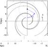 |
Fig. 1 Scheme of the MW plane with the locus 1 (solid) and locus 2 (dashed) employed in the simulations with analytic potentials. The Galaxy rotates clockwise in this picture. |
The initial conditions are generated as detailed in Appendix A from Romero-Gómez et al. (2015), except that here they are two-dimensional. They consist of the Miyamoto-Nagai disk as in the axisymmetric part of the potential. The velocities are approximated as Gaussian distributions, with the dispersion in the radial velocity component decaying as a function of radius with a scale length that is twice that of the density. The azimuthal component is related to the radial component through the epicyclic relation. We also include the asymmetric drift. We use two sets of initial conditions with radial velocity dispersion in the solar neighbourhood σVR(R⊙) of 20 km s-1 (IC20) and 40 km s-1 (IC40).
As the initial conditions are just approximated, stationarity is not guaranteed. To ensure that the system is in steady state and has achieved complete phase mixing, we first integrate the orbits in the axisymmetric potential for 6.1 Gyr. After this, the spiral arms forces are gradually introduced following Eq. (4) of Dehnen (2000) used for a similar purpose but for the Galactic bar. We do this in four revolutions of the arms, which corresponds to 0.9–1.2 Gyr depending on the pattern speed of the model. From the moment that the spiral arms begin to grow, the orbits are integrated for another 14.9 Gyr. Thus, in the integration the spiral arms are fully grown during ~14 Gyr. We note that the MW may not be in a stationary state. Our integration scheme does not try to mimic the evolution of the MW, but aims to obtain a set of final conditions in which the particles are fully phase mixed.
2.2. N-body simulations
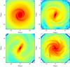 |
Fig. 2 Disk density distribution of models TWA1 (top left), B1 (top right), B5 (bottom left), and U5 (bottom right). |
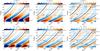 |
Fig. 3 Galactocentric radial VR (top) and azimuthal Vφ (bottom) velocities as a function of cylindrical coordinates for models TWA0, TWA1, and TWA2 (left, middle, and right). Colours show the median velocity in bins in cylindrical coordinates of size ΔR = 0.5 kpc and Δφ = 10°. For Vφ we plot Vφ − ⟨ Vφ ⟩ R where ⟨ Vφ ⟩ R is the average median over all bins at the same radius R, that is we subtract the average rotation velocity at each radius. To make the comparison easier, the colour scale is the same for all panels but the scale indicated above each panel shows only the range for that particular model. The theoretical locus of the arms is shown as a thick black line. The solid and dotted curves indicate the over-density of the spiral arms where the density contrast (N − ⟨ N ⟩ R) / ⟨ N ⟩ R is 0 and 0.2 of the maximum value, respectively, where N is the number of particles in each pixel of the grid and ⟨ N ⟩ R is the azimuthal average. The locations of the main resonances CR, ILR 2:1, ILR 4:1, OLR 4:1, OLR 2:1 are shown with black horizontal lines (solid, dashed, dotted, dashed-dotted, and long-dashed, respectively). The rotation of the Galaxy is towards the left. The black asterisk shows the location of the Sun. |
We use the models B1, B5, and U5 from Roca-Fàbrega et al. (2013, 2014). These are fully self-consistent models with a live exponential disk and live dark matter Navarro Frenk White (NFW) halo, run with the pure N-body adaptive refinement tree (ART) code (Kravtsov et al. 1997). The spatial resolution is 44 pc for B1 and 11 pc for B5 and U5 models. The number of disk particles is 1 million for B1, and 5 million for B5 and U5 models. The differences between B and U models are their initial disk mass (5 × 10¹⁰ and 3.75 × 10¹⁰ M⊙, for B and U models, respectively) and rotation curve. B models have heavier disks and, thus, a similar contribution from the halo and the disk components to the total circular velocity curve. B models develop strong bars in their central regions, which drives the formation of dominant bi-symmetric spiral arms. In the U5 model, the halo contribution is much higher, which prevents the formation of a central barred structure in the first Gyr. The U5 model develops weak multiple-armed structures. The scale length of the disk is 4.2 and 4.1 kpc for B and U models, respectively, and the scale height is 0.2 kpc for both. The stability Toomre parameter Q at solar radius is 3.3 and 1.4, for models B and U, respectively, and >1, thus locally stable, for most of the disk. Details on the initial conditions, initial parameters, and code convergence tests can be found in Roca-Fàbrega et al. (2013).
The top right and bottom panels of Fig. 2 show the disk density of these three models. These models do not necessarily resemble the MW in terms of their rotations curve, total mass, or disk mass, but we use them here as interesting case studies. Model B1 has a bar with a length similar to that of the MW and also a consistent orientation of the spiral arms with respect to the bar that resembles locus 1. The spiral arms of this model rotate at an approximately constant pattern speed at all radii of ~30–40 km s-1 kpc-1. Model B5 does not resemble the MW because it has a bar that is too strong and long and the tangencies of the arms are not consistent with observations, but this model serves as a comparison model. The pattern speed in this case is ~20–25 km s-1 kpc-1. The CR resonance for B1 and B5 is inside the solar radius, contrary to most of our analytic models. U5 corresponds to a galaxy with floculent spiral structure with five major arms that do not rotate with a fixed pattern speed but corotate at the velocity of the disk particles. This is in total opposition to all previous models (both analytic and N-body) and it is an interesting case to be tested for the MW.
For the models B1 and B5, we have oriented the bar at ~20° with respect to the line Sun-Galactic centre (GC), similar to the COBE/DIRBE bar (Gerhard 2002). We orient model U5 to have the Sun between two arms. We also use the case U5b, which is model U5 but for a different orientation of the arms in which the Sun is on top of an arm. In all these simulations we have selected disk particles with height | Z | < 0.6 kpc, which corresponds to 3 scale heights.
2.3. Definitions
We take the location of the Sun at X = 0 and Y = 8.5 kpc, which is indicated with a star in Fig. 1. The Galaxy and the arms rotate clockwise in this plot. Throughout the paper we use Galactocentric cylindrical coordinates R and φ (see convention in Fig. 1) and velocity components VR (positive with increasing R) and Vφ (positive opposite to rotation).
Here we focus on the Gaia observable space and as explained before, on the in-plane components of the velocity. With the usual transformations (e.g. Binney & Merrifield 1998), we turn the simulations into the observables: sky positions l and b, parallax ϖ, los velocity Vlos, and proper motions μl ∗ ≡ μlcosb and μb. For this transformation, we assume that the Sun moves at a peculiar velocity of (U⊙,V⊙,W⊙) = (9,12,7) km s-1 (Dehnen 1998; see discussion in Sect. 4.4) with U positive towards the Galactic centre. We will use the transverse velocity in Galactic longitude VT ≡ kDμl ∗, where k = 4.7404705 km s-1 yrs-1, the distance D is in pc, and μl ∗ is in mas / yr.
3. Spiral arm effects on the stellar velocities
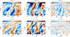 |
Fig. 4 Same as Fig. 3 but for models B1, B5, and U5. The locus of these models is not predefined and thus we only plot the over-density of the spiral arms. The colour scale is the same for all panels but is slightly different from the scale of Fig. 3. |
Figure 3 shows the median galactocentric radial VR (top) and azimuthal Vφ (bottom) velocities as a function of disk position in cylindrical coordinates for models TWA0, TWA1, and TWA2. The rotation of the Galaxy is towards the left part of the plots. In the case of Vφ we subtract the average rotation velocity at each radius (Vφ − ⟨ Vφ ⟩ R). The theoretical locus of the arms is shown as a thick black line. Surrounding the locus, there are solid and dotted curves which indicate the over-density of the spiral arms (see caption). The locations of the main resonances CR, the Inner LR (ILR 2:1, ILR 4:1) and Outer LR (OLR 4:1, OLR 2:1) are shown as black horizontal lines and the position of the Sun is indicated by a black asterisk.
The median VR and Vφ − ⟨ Vφ ⟩ R are expected to be ~0 in an axisymmetric disk. For our models in Fig. 3 these are clearly not null. Moreover, these velocities follow a pattern related to the location of the spiral arms and their main resonances and are different for each of these models. For instance, VR is negative (blue colours) on top of the arms before the CR resonance, it is 0 around CR, and positive (red) beyond. On the other hand, Vφ − ⟨ Vφ ⟩ R is positive in the trailing part of the arm (right of the locus) for most of the radius and negative in the leading part (left). This quantity is null along the locus except inside the ILR 4:1 where it is positive.
For the TWA model, the mean velocities can be estimated analytically (Appendix A3.2 of Roca-Fàbrega et al. 2014). These predictions agree well with our findings above; the main difference is the more abrupt changes of sign in the analytic predictions compared to more gradual changes of sign in the simulations.
Fig. 4 is the same as Fig. 3 but for the N-body models. In these cases the velocity patterns also have a spiral shape but they are related to the arms in a more complex way. For model B1, the inter-arm region seems dominated by negative VR , similar to what happens after CR for the analytic models. This is also the case for model B5 in the regions where the spiral arms, and not the bar, dominate (beyond 6 kpc). For these two models there seems to be a mix of negative and positive values of VR on the spiral arms. For model B1, there is positive Vφ − ⟨ Vφ ⟩ R in the trailing parts of the arms, except for the segment of arm at φ ~ 250°. Model U5 presents tangled velocity patterns, although they also follow some spiral shape. The goal of our study is not to determine the cause of the patterns in these models, but to explore the kinematic features of more complex models.
 |
Fig. 5 Number of particles per bin (top) and transverse velocities VT (bottom) as a function of longitude and distance from the Sun. We have binned this space in bins of Δl = 10° and ΔD = 0.5 kpc. We show the axisymmetric model (left), the TWA1 model (middle), and the difference between these two (right). We superpose the spiral arms locus (black thick line) in these coordinates and the main resonances with curves as in Fig. 3. |
The patterns in velocity that we observe in Figs. 3 and 4 translate into patterns in the Gaia observable space. We present in Fig. 5 several quantities in the longitude-distance plane. The area covered in these plots corresponds to the blue circle in Fig. 1. For the analytic models, we also use the symmetric circle (at Y = −8.5 kpc) to obtain better particle statistics since these models are by definition symmetric. We do not do this with the N-body models since they are not strictly symmetric (Fig. 2). The top row shows the number of particles per bin. We plot here the axisymmetric model (left), that is before the spiral arms are introduced in the simulation, the model TWA1 (middle), and the difference between these two (right). We also plot the spiral arms locus (black thick line), which coincides with the main arm over-densities in the middle and right top panels (red colours).
In the bottom of Fig. 5 we plot the transverse velocity VT. The axisymmetric case (left) and the TWA1 model (middle) do not seem to differ significantly. The effect of the spiral arms only becomes evident in the difference between the two (right). At closer distances (1 kpc) the arms increase the transverse velocity with respect to the axisymmetric case at positive longitudes, and decrease the transverse velocity for negative longitudes. Beyond this distance, the arms and resonances delimit regions of enhanced and reduced VT. For instance, towards the Galactic centre (l = 0°) VT is enhanced at close distances, but it decreases beyond the spiral arm (d ~ 3 kpc), and similarly towards the anti-centre (l = ± 180°). The pattern that we observe here is related to that seen in VR and Vφ since the transverse velocity is a combination of these two. For example, around l = 0° and l = 180°, the VT velocity is mainly −Vφ and Vφ, respectively.
Table 2 quantifies how much the kinematics of the spiral arm models deviate from the axisymmetric case. We only consider here the analytic models for which we have the corresponding axisymmetric model. In Cols. 2 and 3 we show the maximum values of | VT − VT(AXI) | (maximum absolute value in the colour scale of the right bottom panel of Fig. 5) and the median value. In all cases the maximum deviation is at least 10 km s-1 and up to 38 km s-1. In all but one model, 50% of the bins differ from the axisymmetric models by at least 1 km s-1, and in most of the cases by ~2 km s-1. In the final columns we repeat this computation for Vlos velocities, and find very similar values.
Kinematic deviations of the spiral models compared to the axisymmetric models.
Given that the patterns in VR and Vφ, in Figs. 3 and 4, depend on the properties of the spiral arms, the patterns seen in VT are also different for the different models. However, the patterns in VT are not very conspicuous unless we dispose of and subtract the exact axisymmetric model, which is not the case for the real MW. In Sect. 4 we overcome this limitation.
4. Symmetric Galactic longitudes
4.1. The method
Here we compare our simulated data of symmetric Galactic longitudes, that is l and −l, instead of comparing with an axisymmetric model. In particular, we look at the difference between the median transverse velocity VT at symmetric longitudes  (1)For any axisymmetric model, we expect this quantity to be
  (2)This is because the transverse velocities are the same in symmetric longitudes except for the Sun’s motion, which in one direction adds up to the stellar velocity and in the other subtracts from the stellar velocity. However, as seen in the bottom right panel of Fig. 5, the spiral arm models present kinematic features that are not longitude symmetric.
In Fig. 6 we plot the discrepancy between the difference in VT at symmetric longitudes (Δ) and the expected value in an axisymmetric case (Δexp) at each (l,d) bin and its symmetric counterpart at (−l,d) for all of our models, that is Δ−Δexp. In practise, we basically subtract the left part of the bottom middle panel of Fig. 5 from the right part, and then subtract the expected value. We estimate the statistical error on the median VT(l> 0) and VT(l< 0) with bootstrapping. We plot a black cross in bins where the Δ−Δexp is still compatible with 0 with a 75% confidence, i.e. where Δ is compatible with the expected value for an axisymmetric model Δexp. We overplot the locations of the resonances (thin black lines) and the locus of the arms in green and red for the part at positive and negative l, respectively. Figure 7 is equivalent to Fig. 6 but for an axisymmetric model. In this case, we expect Δ−Δexp to be 0 for all bins. This is indeed the case, except for the Poisson fluctuations. In 82% of the bins of this plot, | Δ−Δexp | is smaller than 0.5 km s-1.
 |
Fig. 6 Values of Δ−Δexp as a function of l and D, where Δ ≡ VT (l> 0) − VT (l< 0) is the difference between the median transverse velocity in symmetric bins (l, d) and (−l, d), and Δexp = 2U⊙sinl is the expected value for an axisymmetric model. The first two rows are for simulations with analytic models, and the last row is for N-body models. The colour scale is the same for all panels, except for models B1 and B5 that have higher values. We plot a black cross where the Δ−Δexp is statistically consistent with 0 with a 75% confidence, i.e. where the values of Δ are compatible with an axisymmetric model. The locations of the resonances follow the same line code as Fig. 3. The loci of the spiral arms are indicated in green and red for positive and negative l, respectively. We use the loci estimated in Roca-Fàbrega et al. (2013, 2014) for N-body models B. |
4.2. Comparison of different models
Models in Fig. 6 (with spiral arms) show higher values of Δ−Δexp compared to Fig. 7 (axisymmetric) and present defined patterns. In models TWA0 and TWA1 (first two panels in top row), we expect an excess of transverse velocity for positive l compared to negative l (red) at close distances for all longitudes and at large distances for the range l ~ [ 70,120 ] °. Towards the Galactic centre, we see three changes of sign: at 2 kpc, slightly after crossing the spiral arms, and around the ILR 2:1. In the anti-centre direction, according to these two models, we expect a change of sign around 3 kpc. Models TWA0 and TWA1 have the same configuration of spiral arms, except for their pattern speed which differs by 5 km s-1 kpc-1. Even with this small difference, there are deviations between these two models: model TWA0 has larger perturbations and the last change of sign at l = 0 related to the ILR 2:1 occurs at 4 instead of 5 kpc as in TWA1.
The differences between these two models and TWA2 and TW3 (Fig. 6 third and fourth panels from left in top row) are even more conspicuous. For TWA2 and TWA3, the spiral arms spatial configuration is the same as for TWA0 and TWA1 but the location of the resonances is very different with CR very close to the Sun. In TWA2, for distances up to 4 kpc, this model presents positive and negative values of Δ−Δexp with the limit approximately following the CR resonance. For l ~ 0°, there are now only two changes of sign up to 6 kpc. In TWA3, negative values of Δ−Δexp dominate for all l at nearby distances. We now see different changes of sign associated with the crossing of spiral arms and resonances.
In the second row of Fig. 6 we present Δ−Δexp for the other simulations with the analytic potential (Table 1). The model TWA10 is the same as TWA1 (second panel in top row) but for a double velocity dispersion at the Sun radius. This allows us to see whether a similar kinematic perturbation appears for a hotter (older) population. In TWA11 we reduced the amplitude of the spiral potential. In these two cases the patterns in the velocity do not change compared to TWA1, but present smaller values of Δ−Δexp. As expected, we observe larger kinematic perturbations for model TWA12 with a higher spiral force amplitude. Model TWA13 uses locus 2. In this case, the changes of sign follow the same patterns as in TWA1 but at different distances corresponding to the new location of the arms. For instance, the change of sign at l ~ 180° occurs closer to the Sun, exactly after crossing the arm. While there could be doubt about whether the cause of the sign change at l ~ 180° in models TWA0 and TWA1 was due to the arm crossing or to the resonance crossing (these two features overlap), after inspecting model TWA13, we conclude that the change of sign seems to be due to the former.
Kinematic differences when comparing positive and negative Galactic longitudes in the spiral models.
In the last row of Fig. 6 we show the results for our N-body models. Model B1 presents negative Δ−Δexp for most of the bins with some hints of positive values for small l though statistically not very significant due to the low number of particles in this simulation. Interestingly, the kinematic features in this model resemble model TWA3. These two models have a large pattern speed and even though they have a very different nature, the kinematic effects on the stars look alike. Model B5 shares kinematic similarities with models TWA2 and TWA31, especially the combination of positive and negative values of Δ−Δexp. Model U5 is a multi-arm model that shows messier kinematic patterns that do not resemble any of the previous models, and even has patterns of different intensity inside blue regions. Finally, model U5b, which is the same as U5 but with a different orientation relative to the Sun, is similar to U5 in that it presents complex and smaller scale kinematic features but with a different pattern and sign. We notice here that models U5 and U5b have values of Δ−Δexp that are in the same range of our analytic models. By contrast, models B present much higher values. The interpretation of the panels in the last row is more complex since they include other aspects that influence the disk kinematics apart from the arms (e.g. a bar or a lopsided disk).
Plots such as those in Fig. 6 can be created directly with the Gaia observables and do not require any assumption on the axisymmetric potential of the Galaxy (but see Sect. 4.4). With this advantage, this approach tells us directly about the effects of spiral arms on disk kinematics. Moreover, the comparison with models, such as those shown here, allows us to retrieve properties of the spiral arms of the MW, namely the location of the arms and the main resonances, and thus, the pattern speed, strength, and nature of the arms (grand design versus corotating multi-arm configuration).
In Table 3 we summarise the impact of effects of the spiral arms in symmetric longitudes in the explored region of the disk in the different models. The table shows the distance and longitude of the maximum absolute value of Δ−Δexp (Cols. 2–4), that is the region of the disk surrounding the Sun that deviates more from its symmetric counterpart compared to the axisymmetric expectation. This region happens to be at inner longitudes and at a similar distance for the analytic models, but it is more variable for the N-body models. Columns 5 and 7 show the longitudes with maximum and minimum average | Δ−Δexp |, respectively, and Cols. 6 and 8 indicate the corresponding average | Δ−Δexp |. The Galactic longitude that is globally more affected by the arms is different for all models but the longitudes of 25° and 75° seem recurrent in the analytic models. The direction of the anti-centre is clearly the least affected in the analytic models and in most of the N-body models.
Table 3 also shows the fraction of bins of Fig. 6 (i.e. up to a distance of 6 kpc) that have a value of | Δ−Δexp | larger than 2 km s-1 (Col. 9) and 5 km s-1 (Col. 10). The first fraction is large in most of the models except for TWA2 and TWA11 for which it is around 15%. It is even larger than 60% for some models. But notice that, in the case of TWA11, we decreased the amplitude of the spiral arm force below the estimated ranges for the MW. We also note that model B5, which has most of the bins with a very large value of | Δ−Δexp |, is not comparable to the MW. The fraction of bins with perturbations larger than 5 km s-1 is small for most of the models. In Col. 11 we show the median value of | Δ−Δexp |.
From Table 3 we also see that Δ−Δexp is of the order of 2 km s-1 for an important fraction of the sphere around the Sun and, therefore, a kinematic precision smaller than 1 km s-1 is needed in the measured median VT at each longitude and its symmetric counterpart.
 |
Fig. 8 Same as Fig. 6 but introducing a random relative error in distance of eD = 20% in some models. The colour scale is the same as in Fig. 6. |
 |
Fig. 9 Difference between several kinematic quantities in symmetric bins (l, d) and (−l, d) for model TWA1. The first three plots show the transverse velocity dispersion σ(VT), skewness, and kurtosis of the transverse velocity distribution. The last plot shows the difference between the los velocity Vlos compared to the expected value −2U⊙cosl. We plot a black cross in bins where these quantities are statistically consistent with 0 with a 75% confidence, i.e. where they are compatible with an axisymmetric model. The rest of the notation is as in Fig. 6. |
4.3. Distance error
In Fig. 8 we show several models where we have introduced a random relative error in distance of eD = 20%. They can be compared to the first row of Fig. 6 (without error). In general, the velocity patterns are preserved, but we do observe several introduced biases that we must bear in mind for the future analysis with real data. First, in the models TWA0 and TWA1 with errors, for large values of l, the negative values of Δ−Δexp are now located at closer distances. Thus, this could mislead us to conclude that the spiral arms are closer than they really are in the anti-centre direction, since this is similar to what happens in model TWA13. Model TWA2 is now dominated by blue colours, which would lead us to derive a slightly higher pattern speed. Model TWA3 does not change significantly. We explored the models with different distance errors and conclude that an error of eD = 20% should be our maximum tolerable error in order not to have important biases that dilute the kinematic features.
4.4. The value of U⊙
The effects of the non-axisymmetries are not usually taken into account in the measurement of the solar peculiar velocity. We investigate how much the measured value of U⊙ is affected by the spiral arms in our models. It follows from Eq. (2) that, if we assume that there is no effect of the spiral arms on the kinematics of stars, the comparison of the transverse velocities in symmetric longitudes give us the value of U⊙ = Δ / (2sinl). We computed U⊙ from this formula to each bin in Fig. 6 and subsequently performed the median of all bins (column 12 of Table 3). We also provide the error on the median computed as the dispersion for 1000 bootstraps. The obtained value of U⊙ is different from the true value used in the simulations (U⊙ = 9 km s-1) by at most 2 km s-1 for most of the analytic models. These differences are due to the bias introduced by the arms and not by the statistical error, which is much smaller. If we only use the bins at l = 155°, 165°, and 175°, which are the least affected regions of the disk according to our models (Col. 7), the obtained U⊙ (Col. 13) differs no more than 0.5 km s-1 from the true value. On the contrary, the obtained U⊙ for the N-body models B1 and B5 is significantly different from the true value. We have to keep in mind, however, that the perturbations for these models are very high and other effects such as a lopsided disk could also contribute to these biased values of U⊙.
Ideally, when fitting the data to the models presented here, one should also try to fit for the value of U⊙ or, at least, to include its uncertainty so it can be propagated in the fit. However, in our method, adopting a wrong value of U⊙ would change the term 2U⊙sinl in Eq. (2), which would shift the colour scale of our plots. This would not change the colour patterns in Fig. 6 except if the assumed value of U⊙ is significantly wrong and changes 2U⊙sinl by an amount comparable to the typical values of Δexp−Δ (2 km s-1 or higher). We demonstrated above that, in most cases, it is possible to determine the value of U⊙ with better accuracy.
4.5. Extension of the method
The approach of comparing the kinematics of symmetric longitudes in the Galaxy can be used with quantities other than the median transverse velocity. We show in Fig. 9 the difference in symmetric longitudes between the dispersion, skewness, and kurtosis of the VT distribution. The expected difference of these quantities for an axisymmetric model is 0, but we show that they present patterns related to the location of the arms and main resonances, similar to the median VT. The differences are small but noticeable. In the last panel of Fig. 9 we show the differences between the median los velocity in the symmetric longitudes. In this case, we compute Vlos (l> 0) + Vlos (l< 0) and we subtract the expected value for an axisymmetric model, which is −2U⊙cosl. We see again similar patterns and, in particular, we observe high values up to −40 km s-1, which are even higher than the maximum values seen for the same model for transverse velocities (Fig. 6).
5. Gaia performance
 |
Fig. 10 Number of stars in the GUMS model for three different directions: l = 25° (left), l = 95° (middle) and l = 175° (right) in regions of angular size of Δl = ± 5° and Δb = ± 5°. The top row corresponds to super-giant (dotted lines) and giant (solid) stars, and the bottom row to sub-giant (dotted) and dwarf stars (solid). |
In Sect. 4 we established the conditions for which the signatures of spiral arms can be detected with our new approach of studying symmetric Galactic longitudes. These are: i) a maximum distance error of eD = 20% (Sect. 4.3); and ii) a maximum kinematic error in the determination of Δ−Δexp of 2 km s-1 (Sect. 4.2), which in turn requires an error in the median VT in a single longitude of emed(VT) = 1 km s-1. In this section we estimate whether some Gaia tracers meet these conditions.
To do this, we use the GUMS model that is a simulated catalogue of the sources expected to be observed by Gaia. The Galactic sources (stars) in GUMS are generated based on the Besançon Galactic Model, which includes Galactic thin and thick disks, bulge and halo, based on appropriate density laws, kinematics, star formation histories, enrichment laws, initial mass function, and total luminosities for each of the populations, described in Robin et al. (2012). GUMS gives us the simulated true values for Gaia observables. These are the five astrometric parameters (l, b, ϖ, μl, μb), the los velocity Vlos, and the Gaia photometry (including the GGaia magnitude, and the two broadband magnitudes GBP and GRP). The final Gaia catalogue will also provide atmospheric parameters (metallicity, surface gravity, and effective temperature) and extinction.
The GUMS model includes multiple systems (Arenou 2011). To determine which of these systems will be resolved by Gaia, we use a prescription employed in the Data Processing and Analysis Consortium2. The minimum angular separation on the sky that Gaia can resolve depends on the apparent magnitudes of the stars in the system, and, in the best case, it is ~38 mas. We only consider stars that are resolved for which we have a reliable model for Gaia performance.
To simulate Gaia-like errors for the GUMS sources, we use the code presented in Romero-Gómez et al. (2015)3, updated to the post-launch performance, as described in de Bruijne et al. (2014). The uncertainties on the astrometry, photometry, and spectroscopy are mainly a function of the stellar magnitudes and colours. The geometrical factors and the effect of the scanning law are also taken into account4. Only stars with magnitude G< 20 (the Gaia magnitude limit) are considered. We include the Galactic extinction given by GUMS, which is based on Drimmel et al. (2003).
We extracted from GUMS the stars in three different longitudes, l = 25°,95°, and 175°, in regions of Δl = ± 5° centred in these longitudes and a range in latitude of b = [ 0,5 ] °. We binned the data of these directions in distance with ΔD = 0.5 kpc as in our simulations. Figure 10 shows histograms of the number of stars as a function of true distance (i.e. without errors) in each of the longitudes (columns) for different spectral types (colours) and luminosity classes (rows). We doubled the number of stars to account for the sky region below the Galactic plane b = [ −5,0 ] °. With this we assume that the distribution and properties of stars is the same for b = [ 0,5 ] ° and b = [ −5,0 ] °. Although this is not strictly true since the extinction can vary with latitude, we only aim to estimate of the number of stars observed by Gaia in these directions.
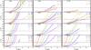 |
Fig. 11 Median relative error in distance as a function of distance for stars in the GUMS model for the different spectral types and luminosity classes for three different directions indicated in the panel labels. We only plot bins with at least ten stars. We use bootstrapping to estimate the error on the median (75% confidence limit), which we indicate with dashed lines. |
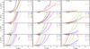 |
Fig. 12 Median error in transverse velocity VT as a function of distance for stars in the GUMS model for the different spectral types and luminosity classes for three different directions indicated in the panel labels. The dashed lines show the 75% confidence limit of the median. |
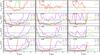 |
Fig. 13 Error in the median transverse velocity VT as a function of distance for stars in the GUMS model for the different spectral types and luminosity classes, and for three different directions indicated in the panel labels. The two horizontal lines show the limits for errors of 1 and 2.5 km s-1. |
As expected, giant and super-giant stars (top row) can be detected up to farther distances. The increase in the number of stars as a function of distance for small distances, subsequent plateau and decrease is due to a combination of aspects. Firstly, our bins, which have a fixed bin ΔD, have a volume that increases with distance. For l = 25° the density of stars also increases with distance because of the density laws of the model. There is a decrease in the number of stars for the same reason for the other directions. The sharp cut-off at around 11 kpc for l = 95° and at 5.5 kpc for l = 175° is due to the size of the disk of the GUMS models with radius of 14 kpc. The stars that are seen beyond those distances are from the halo component. There is a limiting distance for which a star of a certain spectral type can be seen given the magnitude limit of Gaia for dwarf and sub-giant stars (bottom row). In most cases, this limit is not sharp but progressive. This is because of the spread in absolute magnitudes of each spectral type and the different extinction across our fields.
In Fig. 11 we show the median relative error in parallax for the different spectral types and luminosity classes as a function of the true distance for the three longitudes. The differences between the errors in different longitudes are due to extinction, which increases the astrometric errors in the inner fields. We indicate the limit of a relative error eD = 20% with a horizontal line (condition i). To meet this condition, for longitudes of less extinction (l = 95° and l = 175°) we could use giant stars (second row) up to 4 and 6 kpc, depending on the spectral type. The MIII, BIII, and KIII stars are the best tracers in this case. Most of the supergiant stars (top row) also fulfil this condition up to 6 kpc. For l = 25° the high extinction puts the limits for giant stars at 3–4 kpc. For dwarfs stars (bottom row), the limit of eD = 20% is between ~1 and 4 kpc. The OV, BV, AV, and FV stars are the best tracers. Some sub-giant stars also fulfil the distance error condition up to ~2–4 kpc.
We show in Fig. 12 the median error in transverse velocity. These errors influence the precision for which the median VT can be determined. The errors for giant stars are smaller than 5 km s-1 up to ~3–5 kpc, depending on the direction. For dwarf stars this limit is achieved at ~1–4 kpc.
The precision on the determination of the median transverse velocity of a certain population emed(VT) (not to be confused with the median error of the population eVT) depends on the number of observed stars and the dispersion in VT. The latter, in turn, depends on the intrinsic dispersion of the population and the error of the measurements eVT. To estimate the error emed(VT), we compute the median VT of the GUMS velocities after the addition of Gaia-like errors at each bin in distance, and compute its error with the bootstrapping technique. We take the limits of the 75% confidence interval as the error on the median. Since these limits are not necessarily symmetric, we use the maximum absolute difference between the median and the lower or upper limit. We also have to account for the fact that we only extracted the region of b = [ 0,5 ] ° from GUMS. To double the number of stars and thus also include the negative latitude, we assume that the error on the median scales similarly as the error on the mean by a factor  . Also, strictly speaking, this would be the error of the median of the VT in the distribution of the GUMS model. This is not necessarily similar to that shown in our spiral arms models, but we assume that the statistical and measurement errors would yield similar numbers.
In Fig. 13 we show emed(VT). We indicate the error of 1 km s-1 (dotted, condition ii) and, additionally, the error of 2.5 km s-1 (dashed), which correspond to the limit where a signal of Δ−Δexp = 5 km s-1 could be detected with confidence. For super-giant stars (top row), the number of observed stars is too small to fulfil our kinematic condition (emed(VT)< 1 km s-1). For giant stars (second row), the error in the median VT is ≲ 1 km s-1 up to 6 kpc for most of the spectral types except for BIII and MIII stars. For dwarf stars (bottom row), the error is well below 1 km s-1 up to 4 kpc and even beyond for the directions with less extinction, except for B stars. The errors for sub-giants stars happen to be in between giant and dwarf stars and for most of the spectral types (except BIV) the error is emed(VT)< 1 km s-1.
To conclude, we find that the condition of the error in distance (i) necessary for the application of our method to Gaia data is more demanding than the kinematic precision condition (ii). Both conditions are met for most of the spectral types of giant stars up to distances of ~6 kpc (especially KIII stars) and for dwarf stars (especially AV and FV stars) up to closer distances ~3−4 kpc and with better precision (down to 0.5 km s-1), but slightly smaller distances for the longitudes close to l = 0°.
6. Discussion and conclusions
We have shown that comparing the stellar kinematics in symmetric longitudes (i.e. +l and −l) is a useful strategy to put constraints on the properties of spiral arms. We have also seen that the Gaia catalogue will allow us to measure the disk kinematics with enough precision for this approach to be successful.
To do this, we modelled the effects of the arms on the stellar kinematics via controlled orbital integrations in analytic potentials and self-consistent simulations. We studied the trends and magnitudes of the difference between the median transverse velocity as a function of distance in symmetric longitudes. Whereas this difference is expected to be constant and predictable (2U⊙sinl) in an axisymmetric disk, we find that in our models it oscillates in a pattern related to the location of the arms and their resonances. The typical discrepancies between the model values and the axisymmetric predictions are of ~2 km s-1. The detection of this pattern will allow us to quantify the importance of the effect of spiral arms on the orbits of stars in different regions of the disk. Also, it will enable us to put constraints on some properties of the spiral structure, namely the location of the arms, their main resonances and thus, their pattern speed, as well as on their dynamical nature (e.g. grand design versus transient and floculent multiple arms) directly related to the different origin scenarios of spiral structure.
Furthermore, we showed with the GUMS model that the number of stars and the distance and kinematic precision of certain stellar tracers is excellent for detecting the kinematic signatures that we see in the models. With giant stars, we will be able to measure the median transverse velocity with precision smaller than 1 km s-1 up to a distance of ~4–6 kpc and with dwarfs up to ~2–4 kpc and even better kinematic precision (<0.5 km s-1). Although KIII, AIV, AV, and FV stars seem to be the best tracers, an optimum approach would be to examine several spectral types, combined and individually, since each tracer offers different qualities in terms of reached distance and precision. By adding different tracers, we can definitively improve the precision of the measured median transverse velocities, but we must be cautious since different spectral types are composed of populations with different intrinsic dispersions that might have different responses to the potential of spiral arms.
Even more promising, for certain spectral types, we could obtain more precise distances from photometric determinations, e.g. for red clump stars (Bovy et al. 2014), which are also discussed in Romero-Gómez et al. (2015) as good candidate tracers for studies of the Galactic bar. The M0III stars are the stellar tracer chosen in Hunt & Kawata (2014) that allows them to recover the structure and kinematics of the disk with M2M modelling. Although these intrinsically bright stars have the smallest Gaia errors in parallax and proper motions, we find here that their smaller number compared to, for example KIII stars, is not enough to determine the median transverse velocity with the precision sufficient for our approach.
Although there has currently been some effort made in producing good axisymmetric models to describe the MW kinematics, such as in Bienaymé et al. (2015) and Sanders & Binney (2015), our approach does not require the assumption of an axisymmetric model as in previous studies. Our strategy does require, however, knowledge of the value of U⊙. There is currently some debate about this value (Schönrich et al. 2010; Sharma et al. 2014; Huang et al. 2015), which oscillates between 7 and 14 km s-1. Nevertheless, some studies such as Schönrich (2012) presented new methods for measuring the peculiar solar motion that, together with the exceptional Gaia catalogue, are expected to deliver the Sun’s peculiar velocity accurately. However, the kinematic effects of spiral arms are not considered in these methods. Here, with our models we quantified that the determination of U⊙ by a simple median of the velocities in the regions less affected by the arms would yield a value of U⊙ that differs from the true value by less than 0.5 km s-1. We determined that, in all of our models, this is in the direction of the anti-centre (l = 180°). We also checked that assuming a U⊙ that is wrong by ~1 km s-1 would not significantly bias the results obtained with our approach.
A caveat of our study is that we assumed the same extinction in symmetric longitudes. A different extinction would yield different accuracy in parallax and proper motion. This would not create a strong bias, but could compromise the capabilities of detecting the predicted signatures if the extinction in one longitude is much higher than that estimated here. However, a good extinction map will be also a product of the Gaia data and will allow us to evaluate the practical implications of this issue.
Most of the simulations in our study have spiral arms, but no bar. While it is clear that our Galaxy has a bar, this approach allow us to explore the isolated effects of the spiral structure. We are aware that the comparison of the kinematics of symmetric longitudes in real observations will be harder to interpret because of this and other additional effects. A kinematic asymmetry between the first and third quadrant, presumably associated with the effects of the bar, has already been reported in Humphreys et al. (2011). Other effects that we neglect are the passage of satellite galaxies nearby the disk (Quillen et al. 2009) or structures such as the Gould Belt that could distort our maps. We also tested our approach with self-consistent N-body models with the purpose of studying more complete models (for instance including a bar), and we have already seen the complexity that these cases can involve.
We have also seen that the approach of comparing the kinematics of symmetric longitudes could also be useful with other moments of the transverse velocity distribution function such as the dispersion, skewness, and kurtosis, and also with the los velocities. Although it remains to be seen whether these signatures will be detected with statistical significance by Gaia, we will definitively explore this avenue with the data. We also suggest that our proposed approach can be used with surveys of radial velocities such as APOGEE, 4MOST, and WEAVE. The handicap is that these surveys do not cover a wide range or longitudes and their symmetric counterparts. The use of different surveys to compare symmetric longitudes can give rise to additional biases due to differences in the selection function of the surveys or a distance that is difficult to determine, which will need to be evaluated.
Our proposed method can be applied to the second Gaia data release5 scheduled for summer 2017, which will contain the five astrometric parameters for most of the single stars in the final catalogue as well as integrated BP/RP photometry and astrophysical parameters for stars with appropriate standard errors. This release will not enable us to separate the different spectral types completely, but that will be possible with the third release (2017/2018). Earlier searches can be conducted using the Tycho-Gaia astrometric solution (TGAS; Michalik et al. 2015), which will contain proper motions and parallaxes for 2.5 million stars (summer 2016).
Despite the pattern speed of B5 and TWA2 being similar, the location of the resonances of B5 is more similar to TWA3 because of the different rotation curve of these models.
Available at https://github.com/mromerog/gaia-errors.
Acknowledgments
We thank the anonymous referee for his/her comments. T.A. is supported by an ESA Research Fellowship in Space Science.
References
- Allen, C., & Santillan, A. 1991, Mex. Astron. Astrofis., 22, 255 [Google Scholar]
- Antoja, T., Figueras, F., Fernández, D., & Torra, J. 2008, A&A, 490, 135 [NASA ADS] [CrossRef] [EDP Sciences] [Google Scholar]
- Antoja, T., Valenzuela, O., Pichardo, B., et al. 2009, ApJ, 700, L78 [NASA ADS] [CrossRef] [Google Scholar]
- Antoja, T., Figueras, F., Romero-Gómez, M., et al. 2011, MNRAS, 418, 1423 [NASA ADS] [CrossRef] [Google Scholar]
- Antoja, T., Helmi, A., Bienayme, O., et al. 2012, MNRAS, 426, L1 [NASA ADS] [CrossRef] [Google Scholar]
- Antoja, T., Helmi, A., Dehnen, W., et al. 2014, A&A, 563, A60 [NASA ADS] [CrossRef] [EDP Sciences] [Google Scholar]
- Arenou, F. 2011, in AIP Conf. Ser. 1346, eds. J. A. Docobo, V. S. Tamazian, & Y. Y. Balega, 107 [Google Scholar]
- Bienaymé, O., Robin, A. C., & Famaey, B. 2015, A&A, 581, A123 [NASA ADS] [CrossRef] [EDP Sciences] [Google Scholar]
- Binney, J., & Merrifield, M. 1998, Galactic Astronomy (Princeton, NJ: Princeton University Press) [Google Scholar]
- Binney, J., & Tremaine, S. 2008, Galactic Dynamics: Second Edition, eds. J. Binney, & S. Tremaine (Princeton University Press) [Google Scholar]
- Bovy, J., Nidever, D. L., Rix, H.-W., et al. 2014, ApJ, 790, 127 [NASA ADS] [CrossRef] [Google Scholar]
- Bovy, J., Bird, J. C., García Pérez, A. E., et al. 2015, ApJ, 800, 83 [NASA ADS] [CrossRef] [Google Scholar]
- Carlin, J. L., DeLaunay, J., Newberg, H. J., et al. 2013, ApJ, 777, L5 [NASA ADS] [CrossRef] [Google Scholar]
- Churchwell, E., Babler, B. L., Meade, M. R., et al. 2009, PASP, 121, 213 [NASA ADS] [CrossRef] [Google Scholar]
- Contopoulos, G., & Grosbol, P. 1986, A&A, 155, 11 [NASA ADS] [Google Scholar]
- de Bruijne, J. H. J., Rygl, K. L. J., & Antoja, T. 2014, in EAS PS, 67, 23 [Google Scholar]
- De Simone, R., Wu, X., & Tremaine, S. 2004, MNRAS, 350, 627 [NASA ADS] [CrossRef] [MathSciNet] [Google Scholar]
- Debattista, V. P. 2014, MNRAS, 443, L1 [NASA ADS] [CrossRef] [Google Scholar]
- Dehnen, W. 1998, AJ, 115, 2384 [NASA ADS] [CrossRef] [Google Scholar]
- Dehnen, W. 2000, AJ, 119, 800 [NASA ADS] [CrossRef] [Google Scholar]
- Dobbs, C., & Baba, J. 2014, PASA, 31, 35 [Google Scholar]
- Dobbs, C. L., Burkert, A., & Pringle, J. E. 2011, MNRAS, 417, 1318 [NASA ADS] [CrossRef] [Google Scholar]
- Drimmel, R., & Spergel, D. N. 2001, ApJ, 556, 181 [NASA ADS] [CrossRef] [Google Scholar]
- Drimmel, R., Cabrera-Lavers, A., & López-Corredoira, M. 2003, A&A, 409, 205 [NASA ADS] [CrossRef] [EDP Sciences] [Google Scholar]
- Elmegreen, B. G., & Elmegreen, D. M. 1990, ApJ, 355, 52 [NASA ADS] [CrossRef] [Google Scholar]
- Erroz-Ferrer, S., Knapen, J. H., Leaman, R., et al. 2016, MNRAS, 458, 1199 [NASA ADS] [CrossRef] [Google Scholar]
- Famaey, B., Jorissen, A., Luri, X., et al. 2005, A&A, 430, 165 [NASA ADS] [CrossRef] [EDP Sciences] [Google Scholar]
- Faure, C., Siebert, A., & Famaey, B. 2014, MNRAS, 440, 2564 [NASA ADS] [CrossRef] [Google Scholar]
- Font, J., Beckman, J. E., Epinat, B., et al. 2011, ApJ, 741, L14 [NASA ADS] [CrossRef] [Google Scholar]
- Fujii, M. S., & Baba, J. 2012, MNRAS, 427, L16 [NASA ADS] [Google Scholar]
- Gerhard, O. 2002, in The Dynamics, Structure & History of Galaxies: A Workshop in Honour of Professor Ken Freeman, eds. G. S. Da Costa, E. M. Sadler, & H. Jerjen, ASP Conf. Ser., 273, 73 [Google Scholar]
- Gerhard, O. 2011, Mem. Soc. Astron. It. Suppl., 18, 185 [Google Scholar]
- Gieles, M., Athanassoula, E., & Portegies Zwart, S. F. 2007, MNRAS, 376, 809 [NASA ADS] [CrossRef] [Google Scholar]
- Gómez, F. A., Minchev, I., O’Shea, B. W., et al. 2013, MNRAS, 429, 159 [NASA ADS] [CrossRef] [Google Scholar]
- Grand, R. J. J., Kawata, D., & Cropper, M. 2012, MNRAS, 421, 1529 [CrossRef] [Google Scholar]
- Huang, Y., Liu, X.-W., Yuan, H.-B., et al. 2015, MNRAS, 449, 162 [NASA ADS] [CrossRef] [Google Scholar]
- Humphreys, R. M., Beers, T. C., Cabanela, J. E., et al. 2011, AJ, 141, 131 [NASA ADS] [CrossRef] [Google Scholar]
- Hunt, J. A. S., & Kawata, D. 2014, MNRAS, 443, 2112 [NASA ADS] [CrossRef] [Google Scholar]
- Kravtsov, A. V., Klypin, A. A., & Khokhlov, A. M. 1997, ApJS, 111, 73 [NASA ADS] [CrossRef] [Google Scholar]
- Lépine, J. R. D., Roman-Lopes, A., Abraham, Z., Junqueira, T. C., & Mishurov, Y. N. 2011, MNRAS, 414, 1607 [NASA ADS] [CrossRef] [Google Scholar]
- Lin, C. C., Yuan, C., & Shu, F. H. 1969, ApJ, 155, 721 [NASA ADS] [CrossRef] [Google Scholar]
- Martínez-Barbosa, C. A., Brown, A. G. A., Boekholt, T., et al. 2016, MNRAS, 457, 1062 [NASA ADS] [CrossRef] [Google Scholar]
- Michalik, D., Lindegren, L., & Hobbs, D. 2015, A&A, 574, A115 [NASA ADS] [CrossRef] [EDP Sciences] [Google Scholar]
- Minchev, I., & Famaey, B. 2010, ApJ, 722, 112 [NASA ADS] [CrossRef] [Google Scholar]
- Minchev, I., & Quillen, A. C. 2007, MNRAS, 377, 1163 [NASA ADS] [CrossRef] [Google Scholar]
- Minchev, I., & Quillen, A. C. 2008, MNRAS, 386, 1579 [NASA ADS] [CrossRef] [Google Scholar]
- Miyamoto, M., & Nagai, R. 1975, PASJ, 27, 533 [NASA ADS] [Google Scholar]
- Monari, G., Helmi, A., Antoja, T., & Steinmetz, M. 2014, A&A, 569, A69 [NASA ADS] [CrossRef] [EDP Sciences] [Google Scholar]
- Perryman, M. A. C., de Boer, K. S., Gilmore, G., et al. 2001, A&A, 369, 339 [NASA ADS] [CrossRef] [EDP Sciences] [Google Scholar]
- Purcell, C. W., Bullock, J. S., Tollerud, E. J., Rocha, M., & Chakrabarti, S. 2011, Nature, 477, 301 [NASA ADS] [CrossRef] [Google Scholar]
- Quillen, A. C., & Minchev, I. 2005, AJ, 130, 576 [NASA ADS] [CrossRef] [Google Scholar]
- Quillen, A. C., Minchev, I., Bland-Hawthorn, J., & Haywood, M. 2009, MNRAS, 397, 1599 [NASA ADS] [CrossRef] [Google Scholar]
- Reid, M. J., Menten, K. M., Brunthaler, A., et al. 2014, ApJ, 783, 130 [Google Scholar]
- Robin, A. C., Luri, X., Reylé, C., et al. 2012, A&A, 543, A100 [NASA ADS] [CrossRef] [EDP Sciences] [Google Scholar]
- Roca-Fàbrega, S., Valenzuela, O., Figueras, F., et al. 2013, MNRAS, 432, 2878 [NASA ADS] [CrossRef] [Google Scholar]
- Roca-Fàbrega, S., Antoja, T., Figueras, F., et al. 2014, MNRAS, 440, 1950 [NASA ADS] [CrossRef] [Google Scholar]
- Romero-Gómez, M., Figueras, F., Antoja, T., Abedi, H., & Aguilar, L. 2015, MNRAS, 447, 218 [NASA ADS] [CrossRef] [Google Scholar]
- Roškar, R., Debattista, V. P., Quinn, T. R., Stinson, G. S., & Wadsley, J. 2008, ApJ, 684, L79 [NASA ADS] [CrossRef] [Google Scholar]
- Sanders, J. L., & Binney, J. 2015, MNRAS, 449, 3479 [NASA ADS] [CrossRef] [Google Scholar]
- Schönrich, R. 2012, MNRAS, 427, 274 [NASA ADS] [CrossRef] [Google Scholar]
- Schönrich, R., Binney, J., & Dehnen, W. 2010, MNRAS, 403, 1829 [NASA ADS] [CrossRef] [Google Scholar]
- Sellwood, J. A., & Binney, J. J. 2002, MNRAS, 336, 785 [NASA ADS] [CrossRef] [Google Scholar]
- Sharma, S., Bland-Hawthorn, J., Binney, J., et al. 2014, ApJ, 793, 51 [NASA ADS] [CrossRef] [Google Scholar]
- Siebert, A., Famaey, B., Minchev, I., et al. 2011, MNRAS, 412, 2026 [NASA ADS] [CrossRef] [Google Scholar]
- Siebert, A., Famaey, B., Binney, J., et al. 2012, MNRAS, 425, 2335 [NASA ADS] [CrossRef] [Google Scholar]
- Solway, M., Sellwood, J. A., & Schönrich, R. 2012, MNRAS, 422, 1363 [NASA ADS] [CrossRef] [Google Scholar]
- Vallée, J. P. 2008, AJ, 135, 1301 [NASA ADS] [CrossRef] [Google Scholar]
- Vorobyov, E. I., & Theis, C. 2008, MNRAS, 383, 817 [NASA ADS] [CrossRef] [Google Scholar]
- Widrow, L. M., & Bonner, G. 2015, MNRAS, 450, 266 [NASA ADS] [CrossRef] [Google Scholar]
- Widrow, L. M., Gardner, S., Yanny, B., Dodelson, S., & Chen, H.-Y. 2012, ApJ, 750, L41 [NASA ADS] [CrossRef] [Google Scholar]
- Widrow, L. M., Barber, J., Chequers, M. H., & Cheng, E. 2014, MNRAS, 440, 1971 [NASA ADS] [CrossRef] [Google Scholar]
- Williams, M. E. K., Steinmetz, M., Binney, J., et al. 2013, MNRAS, 436, 101 [NASA ADS] [CrossRef] [Google Scholar]
All Tables
Kinematic differences when comparing positive and negative Galactic longitudes in the spiral models.
All Figures
|
Fig. 1 Scheme of the MW plane with the locus 1 (solid) and locus 2 (dashed) employed in the simulations with analytic potentials. The Galaxy rotates clockwise in this picture. |
| In the text | |
|
Fig. 2 Disk density distribution of models TWA1 (top left), B1 (top right), B5 (bottom left), and U5 (bottom right). |
| In the text | |
|
Fig. 3 Galactocentric radial VR (top) and azimuthal Vφ (bottom) velocities as a function of cylindrical coordinates for models TWA0, TWA1, and TWA2 (left, middle, and right). Colours show the median velocity in bins in cylindrical coordinates of size ΔR = 0.5 kpc and Δφ = 10°. For Vφ we plot Vφ − ⟨ Vφ ⟩ R where ⟨ Vφ ⟩ R is the average median over all bins at the same radius R, that is we subtract the average rotation velocity at each radius. To make the comparison easier, the colour scale is the same for all panels but the scale indicated above each panel shows only the range for that particular model. The theoretical locus of the arms is shown as a thick black line. The solid and dotted curves indicate the over-density of the spiral arms where the density contrast (N − ⟨ N ⟩ R) / ⟨ N ⟩ R is 0 and 0.2 of the maximum value, respectively, where N is the number of particles in each pixel of the grid and ⟨ N ⟩ R is the azimuthal average. The locations of the main resonances CR, ILR 2:1, ILR 4:1, OLR 4:1, OLR 2:1 are shown with black horizontal lines (solid, dashed, dotted, dashed-dotted, and long-dashed, respectively). The rotation of the Galaxy is towards the left. The black asterisk shows the location of the Sun. |
| In the text | |
|
Fig. 4 Same as Fig. 3 but for models B1, B5, and U5. The locus of these models is not predefined and thus we only plot the over-density of the spiral arms. The colour scale is the same for all panels but is slightly different from the scale of Fig. 3. |
| In the text | |
|
Fig. 5 Number of particles per bin (top) and transverse velocities VT (bottom) as a function of longitude and distance from the Sun. We have binned this space in bins of Δl = 10° and ΔD = 0.5 kpc. We show the axisymmetric model (left), the TWA1 model (middle), and the difference between these two (right). We superpose the spiral arms locus (black thick line) in these coordinates and the main resonances with curves as in Fig. 3. |
| In the text | |
|
Fig. 6 Values of Δ−Δexp as a function of l and D, where Δ ≡ VT (l> 0) − VT (l< 0) is the difference between the median transverse velocity in symmetric bins (l, d) and (−l, d), and Δexp = 2U⊙sinl is the expected value for an axisymmetric model. The first two rows are for simulations with analytic models, and the last row is for N-body models. The colour scale is the same for all panels, except for models B1 and B5 that have higher values. We plot a black cross where the Δ−Δexp is statistically consistent with 0 with a 75% confidence, i.e. where the values of Δ are compatible with an axisymmetric model. The locations of the resonances follow the same line code as Fig. 3. The loci of the spiral arms are indicated in green and red for positive and negative l, respectively. We use the loci estimated in Roca-Fàbrega et al. (2013, 2014) for N-body models B. |
| In the text | |
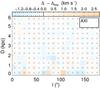 |
Fig. 7 Same as Fig. 6 but for an axisymmetric model. |
| In the text | |
|
Fig. 8 Same as Fig. 6 but introducing a random relative error in distance of eD = 20% in some models. The colour scale is the same as in Fig. 6. |
| In the text | |
|
Fig. 9 Difference between several kinematic quantities in symmetric bins (l, d) and (−l, d) for model TWA1. The first three plots show the transverse velocity dispersion σ(VT), skewness, and kurtosis of the transverse velocity distribution. The last plot shows the difference between the los velocity Vlos compared to the expected value −2U⊙cosl. We plot a black cross in bins where these quantities are statistically consistent with 0 with a 75% confidence, i.e. where they are compatible with an axisymmetric model. The rest of the notation is as in Fig. 6. |
| In the text | |
|
Fig. 10 Number of stars in the GUMS model for three different directions: l = 25° (left), l = 95° (middle) and l = 175° (right) in regions of angular size of Δl = ± 5° and Δb = ± 5°. The top row corresponds to super-giant (dotted lines) and giant (solid) stars, and the bottom row to sub-giant (dotted) and dwarf stars (solid). |
| In the text | |
|
Fig. 11 Median relative error in distance as a function of distance for stars in the GUMS model for the different spectral types and luminosity classes for three different directions indicated in the panel labels. We only plot bins with at least ten stars. We use bootstrapping to estimate the error on the median (75% confidence limit), which we indicate with dashed lines. |
| In the text | |
|
Fig. 12 Median error in transverse velocity VT as a function of distance for stars in the GUMS model for the different spectral types and luminosity classes for three different directions indicated in the panel labels. The dashed lines show the 75% confidence limit of the median. |
| In the text | |
|
Fig. 13 Error in the median transverse velocity VT as a function of distance for stars in the GUMS model for the different spectral types and luminosity classes, and for three different directions indicated in the panel labels. The two horizontal lines show the limits for errors of 1 and 2.5 km s-1. |
| In the text | |
Current usage metrics show cumulative count of Article Views (full-text article views including HTML views, PDF and ePub downloads, according to the available data) and Abstracts Views on Vision4Press platform.
Data correspond to usage on the plateform after 2015. The current usage metrics is available 48-96 hours after online publication and is updated daily on week days.
Initial download of the metrics may take a while.