| Issue |
A&A
Volume 699, July 2025
|
|
|---|---|---|
| Article Number | A269 | |
| Number of page(s) | 20 | |
| Section | Galactic structure, stellar clusters and populations | |
| DOI | https://doi.org/10.1051/0004-6361/202453444 | |
| Published online | 16 July 2025 | |
Open clusters in the outer disc studied with GTC/MEGARA
Auner 1 and Berkeley 102
1
Institut d’Estudis Espacials de Catalunya (IEEC),
Gran Capità 2–4,
08034
Barcelona,
Spain
2
Institut de Ciències del Cosmos (ICCUB), Universitat de Barcelona (UB),
Martí i Franquès, 1,
08028
Barcelona,
Spain
3
Departament de Física Quàntica i Astrofísica (FQA), Universitat de Barcelona (UB),
Martí i Franquès, 1,
08028
Barcelona,
Spain
4
INAF – Osservatorio di Astrofisica e Scienza dello Spazio di Bologna,
via Gobetti 93/3,
40129
Bologna,
Italy
5
Observatoire de Paris (Meudon)
GEPI Batiment 11, Hipparque 5 Place Jules Janssen,
92195
Meudon,
France
6
Departamento de Física de la Tierra y Astrofísica, Universidad Complutense de Madrid,
Plaza Ciencias, 1,
28040
Madrid,
Spain
7
IPARCOS (Instituto de Física de Partículas y del Cosmos), Facultad de Ciencias Físicas, Ciudad Universitaria,
Plaza de las Ciencias, 1,
Madrid
28040,
Spain
★ Corresponding author: This email address is being protected from spambots. You need JavaScript enabled to view it.
Received:
13
December
2024
Accepted:
10
June
2025
Abstract
Context. Open clusters provide valuable information on stellar nucleosynthesis and the chemical evolution of the Galactic disc because their age and distances can be measured more precisely than for field stars.
Aims. We study the outermost parts of the Milky Way disc using open clusters as tracers. We focus on two clusters at galactocentric distances of about 14 kpc that have never been spectroscopically observed before and are located in largely unexplored regions of the Galaxy.
Methods. We used medium-resolution spectra (R > 18 700) obtained with the MEGARA integral-field unit (IFU) spectrograph at the 10.4 m Gran Telescopio Canarias (GTC) to study red giant star members of the clusters Auner 1 and Berkeley 102. We determined the radial velocities and atmospheric parameters for the member stars, and we updated the ages and distances for these two clusters. Finally, we measured the abundances of six chemical elements, that is, Fe, Ca, Co, Ni, Ba, and Eu.
Results. The two clusters are both old, 3.2 ± 0.7 Ga, are distant, d ~ 8 kpc, and are moderately affected by interstellar extinction, AV ~ 1.3 mag, because they are located below the Galactic mid-plane, ZGal ~ −0.7 kpc. The metallicities of Auner 1, [Fe/H]= −0.30 ± 0.09, and Berkeley 102, [Fe/H]= −0.35 ± 0.06, are compatible with the values of other open clusters that are situated at similar galactocentric radii. This suggests that the azimuthal metallicity varies little. The relative abundance ratios, [X/Fe], also behave as expected, perhaps with the exception of [Ca/Fe], which appears to be slightly enhanced in both clusters, and [Eu/Fe], which is enhanced in Berkeley 102, [Eu/Fe] = 0.64 ± 0.05.
Conclusions. Our results demonstrate that competitive Galactic archaeology is possible with GTC/MEGARA observations in IFU mode. The two studied objects open a new window into the chemical evolution of the outer Galactic disc. More observations of distant (in galactocentric distance and azimuth) open clusters with medium- to high-resolution instruments on 8-10 m-class telescopes are needed to firmly establish the abundance trends of the outermost parts of the Galactic disc.
Key words: stars: abundances / Galaxy: abundances / Galaxy: disk / Galaxy: evolution / open clusters and associations: general
© The Authors 2025
 Open Access article, published by EDP Sciences, under the terms of the Creative Commons Attribution License (https://creativecommons.org/licenses/by/4.0), which permits unrestricted use, distribution, and reproduction in any medium, provided the original work is properly cited.
This article is published in open access under the Subscribe to Open model. This email address is being protected from spambots. You need JavaScript enabled to view it. to support open access publication.
1 Introduction
Open clusters (OCs) are found at all ages and throughout the disc. They serve as excellent tracers of the overall history of star formation and nucleosynthesis throughout the lifetime of the Galactic disc (Friel 2013). This is because OC ages and distances can be measured more accurately than other tracers, such as field stars. OCs have been used to trace the spatial distribution of the metallicity in the Galactic disc. The first studies reported a significant decrease in the metallicity with increasing galactocentric radius, which seems to flatten at a certain distance (e.g. Carrera & Pancino 2011). It shows a knee at intermediate distances (e.g. Magrini et al. 2009; Yong et al. 2012). Recent homogeneous studies based on large spectroscopic surveys, GES (Gaia ESO Survey, Magrini et al. 2022), APOGEE (Apache Point Observatory Galactic Evolution Experiment, Myers et al. 2022), GALAH (GALactic Archaeology with HERMES, Spina et al. 2021), and the compilation OCCASO+ (Open Clusters Chemical Abundances from Spanish Observatories, Carbajo-Hijarrubia et al. 2024), showed that the position of the knee is located between RGC~11 kpc and RGC~12 kpc. Nevertheless, only 8 of the 187 OCs in which more than one star was spectroscopically observed at a resolution R > 20 000 were studied in the outer part of the Galactic disc (RGC > 14 kpc). This prevents a precise characterization of this change in the gradient. It is difficult to determine the abundances for the outer disc OCs because they are located at large distances, and therefore, the brightness of their stars is faint. It reaches G > 15 mag.
In addition to OCs, several other tracers have been used to study the metallicity gradient, such as H II regions (e.g., Balser et al. 2011; Arellano-Córdova et al. 2020; Méndez-Delgado et al. 2022), planetary nebulae (e.g. Maciel et al. 2007; Stanghellini & Haywood 2018), Cepheids (e.g. Genovali et al. 2014; Luck 2018; Minniti et al. 2020; da Silva et al. 2022), low-mass main-sequence stars (e.g. Boeche et al. 2014; Anders et al. 2017), and massive stars (e.g. Daflon & Cunha 2004; Bragança et al. 2019). In almost all cases, a continuously decreasing slope was found that lacked a knee, except in the recent work of da Silva et al. (2023), which was focused on the study of Cepheids.
We obtained observations made with the 10.4 m Gran Telescopio Canarias (GTC) and the MEGARA instrument in one of its high-resolution modes at R ~ 18 700. Based on these, we provide a study of two OCs in the outer disc, Auner 1 and Berkeley 102. The two clusters have not been studied spectroscopically and are located at very different Galactic azimuths (see Table 2).
The goal of this paper is to study the kinematics of the two clusters and their elemental chemical abundances and to analyse their metallicities and abundances in the context of the trends derived with other clusters. In this way, we demonstrate that competitive Galactic archaeology observations with GTC/MEGARA are possible. The paper is organised as follows. The observations and method are described in Sect. 2. We describe the determination of radial velocities and kinematics in Sect. 3 and the abundance determination in Sect. 4. The Galactic trends are described in Sect. 5. Finally, we discuss our conclusions in Sect. 6.
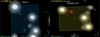 |
Fig. 1 Spatial distribution in the field of the IFU. We mark the stars that were observed inside the field of view of MEGARA with squares. |
2 Observations and method
2.1 Instrumentation
MEGARA is an integral-field unit (IFU) and multi-object spectrograph (MOS) installed at the 10.4 m GTC at the Roque de los Muchachos Observatory on the island of La Palma (Spain) (Gil de Paz et al. 2018; Carrasco et al. 2018). MEGARA has 18 diffraction gratings, 6 of which are in low resolution (R ~ 6000), 10 are in medium resolution (R ~ 12 000), and 2 in high resolution (R ~ 18700). They each cover a different spectral range. These characteristics are the same in IFU and MOS modes.
The IFU consists of 567 contiguous hexagonal fibres with a diagonal of 0.62 arcsec each, encapsulated in a hexagonally packed rectangular shape. This results in a field of view of ~12.54 × 11.3 arcsec2. The instrument has eight fibre bundles that are located in the outer parts of the focal plane, away from the IFU. Simultaneous observations of the sky using 56 hexagonal fibres are possible in this way.
We selected the HR-R volume-phase holographic (VPH) grating, whose resolution of R ~ 18700 and coverage of the spectral range 640.56-679.71 nm allowed us to study the lines of Fe, Ca, Ti, Co, Ni, Ba, and Eu. Unfortunately, the MEGARA MOS mode was not available during the periods 2022A and B.
We therefore conducted the study with the IFU mode alone. This limited the number of stars that could be studied per cluster in a single pointing compared with the better-suited capabilities of the MOS mode.
2.2 Observational strategy
We selected the pointings of the OCs in order to observe three red giant branch (RGB) or red clump (RC) stars in the IFU field of view using the members of the catalogue compiled by Cantat-Gaudin et al. (2020)1 (Fig. 1). The selection of RC stars followed the criterion that they were in the same evolutionary stage to avoid the variation in the abundances between stars that are caused by stellar evolution or atomic diffusion. The difference in the evolutionary stage between RC and RGB stars does not imply a change in the abundances for the elements under study. The RC and RGB stars can easily be identified even in sparsely populated colour-magnitude diagrams (CMDs). They are also brighter than main-sequence stars, which allowed us to observe them at larger heliocentric distances. As the selected stars are hotter than the brighter giants, their spectra are less crowded with lines. This allowed us to determine the atmospheric parameters (effective temperature, surface gravity, and metallicity) and chemical abundances more precisely. The observed stars have high astrometric membership probabilities (Cantat-Gaudin et al. 2020; Hunt & Reffert 2024) derived from Gaia EDR3 (Gaia Collaboration 2021b).
Auner 1 was observed in seven observing blocks (OBs), each with four exposures of 1000 s (proposal ID: GTC93-22B). This amounted to a total of 9.57 h of observation (taking the overheads per pointing time into account). This allowed us to obtain spectra with a high enough signal-to-noise ratio (S/N > 40) for deriving the chemical abundances of three stars with a magnitude G between 16 and 17 (Fig. 2 and Table 1). Another star belonging to the cluster was also observed in two of the OBs. The S/N obtained from these two OBs was sufficient to determine υrad, but it was not high enough to measure its chemical abundance.
Berkeley 102 was observed in four OBs following the same strategy as for Auner 1 (proposal ID: GTC92-22A). This amounted to a total of 5.5 h of observation and included the pointing time and overheads. In this cluster, we observed three stars with magnitudes G ~ 16.2 (Fig. 2).
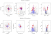 |
Fig. 2 Sky positions, proper motions, parallax vs. magnitude, and CMD of Auner 1 (top panels) and Berkeley 102 (bottom panels). We show all the stars in the region (black points) and the stars that were considered members of each cluster by Cantat-Gaudin et al. (2020) (red circles) and Hunt & Reffert (2024) (blue circles). We mark the observed stars with orange squares. |
Details of the observed stars.
2.3 Data reduction
The raw IFU spectra of the two OCs were reduced using the MEGARA data reduction pipeline (MDRP, Pascual et al. 2024). We started by removing the level of bias present in the image. To remove this value from the counts in the images, we used bias images taken during the corresponding observing night and the task MegaraBiasImage. Faulty pixels are automatically masked in this step with the file master_bpm.fits, which is available at MDRP. The spectra were then processed using the Trace and ModelMap tasks, tracing the fibre spectra through the halogen-lamp images. MDRP was used to perform the wavelength calibration of the spectra using ThNe calibration-lamp images. Using MDRP, we performed a fiber-flat correction using the same halogen-lamp images. We combined the calibrated exposures of each OB using the median and rejected cosmic rays in the process. In addition, MDRP subtracts the mean spectrum of the sky as determined by the spectra of the dedicated fibres to generate the fully reduced spectra. For each OB, we selected all the spaxels on which the signal from the corresponding star was clearly seen above the noise. For this purpose, we used the MEGARA QLA code (Gómez-Álvarez et al. 2018). This implied that for the range of seeing of our observations (between 0.7 and 1.6), we had to extract two rings of hexagonally shaped and packed spaxels around the brightest spaxel on which the star was centred, or 1+6+12=19 spaxels per star.
The following processing steps were performed using the code iSpec (Blanco-Cuaresma et al. 2014). We combined spectra belonging to the same star observed in different OBs. We determined the continuum level of the real spectra by comparing it with a synthetic reference spectrum generated with iSpec and then normalising it. We used the radiative transfer code and line list described in Sect. 4. The reference spectra were computed using the Teff and log g taken from the StarHorse catalogue (Anders et al. 2022b, Table 1), and the metallicity was fixed for all stars to an estimate for the galactocentric radius of the clusters ([M/H]=−0.2 dex). This process was made in conjunction with the determination of the vrad of the star, as detailed in Sect. 3. StarHorse derived the stellar properties with the photo-astrometric information of Gaia EDR3, combined with the photometric catalogues of Pan-STARRS1 (Chambers et al. 2016), SkyMapper (Onken et al. 2019), 2MASS (Cutri et al. 2003), and AllWISE (Cutri et al. 2013).
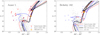 |
Fig. 3 Colour-magnitude diagram of Auner 1 (right) and Berkeley 102 (left). Stars in the field are marked as grey dots, and those that were considered members by Cantat-Gaudin et al. (2020) are shown as red circles and those by Hunt & Reffert (2024) as blue circles. We also mark the observed stars with orange squares (those in Berkeley 102 overlap). We superimpose the isochrone fitting of Cantat-Gaudin et al. (2020) (red), Hunt & Reffert (2024) (blue), and ours (black). |
3 Cluster parameters and kinematics
3.1 Redetermination of the distances and ages
We began by redetermining the astrophysical parameters of the clusters in order to obtain more accurate distances and ages. We followed the method described by Anders et al. (2022a). Although the list of members of Hunt & Reffert (2024) is based on Gaia DR3 and the list by Cantat-Gaudin et al. (2020) is based on Gaia DR2, the stars that we observed belong to both lists. Thus, both works considered our stars as members of the clusters with a high probability (Fig. 2). Using the Hunt & Reffert (2024) members, we first redetermined the zero-point-corrected cluster parallaxes. We calculated the parallax zero-point for all stars in the field (following Lindegren et al. 2021), applied this correction to the member stars, and then determined the corrected mean parallax (and its uncertainty) for the two clusters as  mas and
  mas.
mas.
We also calculated the Bayesian distances to the clusters, assuming negligible parallax correlations, a zero-point uncertainty of 0.005 mas, and a negligible cluster extent (compared to the distance). We obtained  kpc and
  kpc.
kpc.
We redetermined the interstellar extinction towards the two clusters using the results from StarHorse for Gaia EDR3 stars (Anders et al. 2022b), cross-matched with the membership catalogue of Hunt & Reffert (2024). We derived extinctions of AVAuner1 = 1.35 ± 0.03 mag and AVBe102 = 1.32 ± 0.12 mag, respectively. After we precisely determined the extinction and distance and with the metallicity derived from MEGARA spectra (see Sect. 4), we revisited the cluster CMD and adjusted the PARSEC 2.0 isochrones (Nguyen et al. 2022) to determine the best-fitting ages of the two objects (see Fig. 3). In both cases, an isochrone with log age = 9.5 resulted in the best fit of the blue edge of the main sequence, main-sequence turn-off, and red clump. We estimated the uncertainty in these visual fits to be about 0.1 dex in log age (see dashed lines in Fig. 3), and we therefore obtained an age of 3.2 ± 0.7 Ga for the two clusters. The physical parameters for Auner 1 and Berkeley 102 are summarised in Table 2.
3.2 Measurement of the radial velocity
MEGARA is not thermally stabilised, and the wavelength calibration might therefore vary slightly. This affects the radial velocity determination. To characterise these variations, we used the sky spectra obtained in each OB. Based on the sky emission line list of Hanuschik (2003), we prepared a synthetic sky spectrum based on UVES spectra with the resolution and spectral range of the MEGARA HR-R VPH grating. With the 24 available lines, we calculated the vrad differences of each OB with respect to the reference spectrum by cross-correlating it with iSpec. The typical differences between the observations are about 2.0 ± 0.7 km s−1 and reach a maximum of 6.5 ± 0.7 km s−1. Each OB was corrected for the differences we identified. We verified that this improves the RV accuracy by a factor of ten by comparing the dispersion of the results with and without this procedure.
After we refined the wavelength calibration, we applied the heliocentric correction to the spectra. We measured the velocity difference between the OBs with a cross-correlation and used the observation with the highest S/N as reference. We corrected for the differences in vrad and combined the spectra. In this step, we also measured the dispersion in the measurements of vrad of each OB (vscatter) and took the low statistics correction factor in σ into account by applying equation 5 of Roesslein et al. (2007). We also derived the uncertainty in the determination of vrad with a cross-correlation with the reference spectrum (verr). We determined the radial velocity of the combined spectrum with iSpec with a cross-correlation with the same reference spectra as we used in the normalisation process. We verified that by using a reference spectrum with the metallicity measured in Sect. 4, we obtained the same value of vrad. The results are presented in Table 1.
In the cases of stars Berkeley 102_1, Auner 1_1, and Auner 1_2, the value of vscatter is higher than that of the other stars. The S/N values are not low enough to explain these differences. The vscatter values for these stars might be representative of the uncertainties, although they might also be a sign of binarity. Because no spectral lines of companion stars were detected in the spectra, we also used these stars to determine the chemical abundances in Sect. 4. When we do not consider the star with the highest vscatter, the mean value of vscatter is 770 ms−1. Berkeley 102_2 has a considerably different value of vrad than the other two observed stars. The membership of this star should be reviewed when the vrad of more stars in the cluster is measured. We find the vrad of the other observed stars to be compatible with each other, which confirms that they are member stars of the respective clusters.
Properties of the two clusters.
3.3 Membership and mean radial velocity of the clusters
To determine the radial velocity of the cluster, vrad,OC, we used a weighted average, following the same procedure as described by Soubiran et al. (2018). The mean vrad,OC was obtained using
 (1)
(1)
where vrad,i is the radial velocity of each star in the cluster, and the weight wi was defined as wi = 1/(vscatter,i)2.
Similarly, the internal velocity dispersion was derived as
 (2)
(2)
Finally, the uncertainty in the mean vrad,OC, evrad,OC, was defined as the maximum of the standard error,  , and
, and  (Jasniewicz & Mayor 1988), where N is the number of member stars and I is the internal error of vrad,OC, defined as
 (3)
(3)
The values obtained are listed in Table 2. vrad is determined here for the first time for these clusters.
To investigate the kinematics of the clusters in the context of the Galactic disc, we studied the radial velocity of the OCs along with the proper motions, distances, and ages given in Table 2. We used the mean proper motions from Hunt & Reffert (2024) based on Gaia DR3 data.
3.4 Radial velocity with respect to GSR and RSR
We calculated the line-of-sight velocity with respect to the galac-tocentric standard of rest (GSR) and with respect to the regional standard of rest (RSR), using the following equations:
 (4)
(4)
 (5)
(5)
where vrad,OC is the mean heliocentric radial velocity of the cluster, derived in the previous Sect. 3.3. (U⊙, V⊙, W⊙) are the components of the motion of the Sun with respect to the local standard of rest (LSR), and Θ0 and ΘR are the circular velocities at the galactocentric distances from the Sun (R0) and the cluster (RGC), respectively. For the Sun, we adopted (U⊙, V⊙, W⊙) = (11.1, 12.24, 7.25) km s−1, as obtained by Schönrich et al. (2010) and R0 = 8.34 kpc derived in Reid et al. (2014). As the circular velocity around the Galactic centre, we adopted Θ0= 240 km s−1 from Reid et al. (2014), and ΘR was calculated according to the Galactic potential described below in Sect. 3.5.
The results are listed in Table 2. The uncertainties were estimated with 100 000 random draws from uncorrelated Gaussian uncertainties, and we took the errors in the radial velocities and cluster distances into account. The two clusters show values of vRSR that are typical of clusters with thin-disc kinematics (Carrera et al. 2022).
We derived the full spatial velocities with respect to the GSR (VR, Vφ, Vz) and RSR (Us, Vs, Ws) as US = VR, VS = Vφ - ΘR and Ws = Vz. These values are also included in Table 2. Figure 4 shows the projection onto the Galactic plane of the position and velocity with respect to the RSR of the clusters in our sample, in addition to those studied by Carrera et al. (2022), which are included for comparison. We also represent the spiral arms determined by Reid et al. (2019). Auner 1 and Berkeley 102 have peculiar velocities that are compatible with the kinematics of the thin disc, as we also determined when we studied their vRSR.
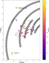 |
Fig. 4 Projection onto the Galactic plane of the position and velocity with respect to the RSR of our two clusters (squares) and Carrera et al. (2022) (circles), coloured by age. We also depict the spiral arms determined by Reid et al. (2019). |
3.5 Orbital analysis
To complete our analysis, we integrated the orbits of Auner 1 and Berkeley 102. Due to the uncertainty in the characterisation of the real Galactic potential, we considered four models that were proposed in the literature. The model proposed by Bovy (2015), denoted MW2014, is an axisymmetric potential composed of a spherical bulge, a Miyamoto-Nagai disc, and a halo with a Navarro-Frenk-White profile (Navarro et al. 1997). The second and third models are based on the first model, but two non-axisymmetric components are added. For the second model, we added a bar characterised by a Ferrers’ potential (Ferrers 1877) with n = 2, and the semi-major, semi-medium, and semi-minor axes were set to 3 kpc, 0.35 kpc, and 0.2375 kpc, respectively; the mass of the bar was 1010 M⊙ (Romero-Gómez et al. 2015), and a constant velocity pattern was set at Ω = 42 km s−1 kpc−1 (Bovy et al. 2019), which placed the corrotation at RGC = 5.6 kpc and the outer Lindblad resonance at RGC = 9 kpc. The angular orientation of the bar with respect to the Sun-Galactic centre line was 20o (see Romero-Gómez et al. 2011, and references therein). The third model adds sinusoidal spiral arms of Cox & Gómez (2002) to the axisymmetric potential. We modelled two spiral arms with an amplitude of 0.1 and a velocity pattern of Ω = 21 km s−1 kpc−1 (e.g., Antoja et al. 2011), which placed the corrotation at RGC = 10.6 kpc. The fourth model is the sum of the axisymmetric potential with the bar and arms described above. Using the package Python galpy (Bovy 2015), we integrated the orbit backwards in time over the cluster age, with a step of 2 Ma. The components of the motion of the Sun with respect to the LSR, the galactocentric distance from the Sun, the circular velocity at this distance, and the distances and ages of the OCs are as described in Sect. 3.4.
Oribt calculations for old clusters have large uncertainties that increase the farther back in time the orbit is determined because we do know the temporal evolution of the potential or the interaction of the clusters with structures in the disc, such as molecular clouds. To calculate the uncertainties of the orbital parameters, we analysed each orbit for the possible values of each of the input parameters, and we took their uncertainties into account. We used 1000 realisations of Monte Carlo sampling values and integrated the orbits. We show the most probable orbits of the two clusters assuming the potentials MW2014, MW2014+bar, and MW2014+arms in the X-Y and RGC-Z planes (Fig. 5), and we list the orbital parameters we computed with all the potential in Table A.3.
We explored the parameters that can be fitted to the potential. One of these parameters is the amplitude of the arm potential (Cox & Gómez 2002). This factor indicates the importance of the arm potential with respect to the axisymmetric potential. The value used in the Cox & Gómez (2002) standard model is 40%. This value yields large displacements in Z for Auner 1 and Berkeley 102 and high eccentricities of about 0.3. Although an arm amplitude of 40% may fit other galaxies well, an assumed arm amplitude of 10% agrees better with the literature values for the Milky Way and produces orbits that are more similar to those calculated with the other potentials. The orbits computed with the different potentials (including those amusing spiral arm potential with a 10% amplitude) are the orbits expected for objects in the thin disc (Carrera et al. 2022, see Fig. 5). From Gaia Collaboration (2021a), based on Gaia EDR3 data (Gaia Collaboration 2021b), we know that the orbits of other two outer disc OCs, Saurer 1 and Berkeley 29, are also typical of thin-disc objects.
Figure 6 shows the dependence of zmax (top) and of the eccentricity (bottom) on the age and RGC (colour-coded). The orbits were calculated with the potential MW2014 + bar + arms. This figure compares the results of Auner 1 and Berkeley 102 with those of the OCCASO sample (Carrera et al. 2022). Similar results were obtained using only the MW2014 potential and including the bar and spiral arms separately. Regardless of the chosen potential, the two clusters observed with MEGARA have higher values of zmax than OCs with similar ages. This is because they are in the outer disc, where the Galactic potential is weaker, and where the orbits therefore reach higher zmax values more easily (Cantat-Gaudin et al. 2020). The eccentricity of the clusters we studied in the outer disc is within the range of eccentricities expected for their age when compared to the OCCASO sample.
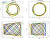 |
Fig. 5 Orbits of Auner 1 (left) and Berkeley 102 (right) for potentials MW2014 (blue), MW2014 + arms (green), and MW2014 + bar (yellow). |
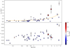 |
Fig. 6 Dependence of the orbital parameters zmax (top) and eccentricity (bottom) on the age and galactocentric radius of OCs. In the top panel, we fit the data with an exponential function. Objects observed with MEGARA are marked with circles, and objects observed with OCCASO (Carrera et al. 2022) are shown as triangles. In all of them, the galactocentric radius is colour-coded. |
4 Abundance determination
We used spectral synthesis with iSpec to determine the atmospheric parameters and chemical abundances. The radiative transfer code we chose was SPECTRUM, and we used the MARCS stellar atmospheric model. We used the sixth version of the GES line list (Heiter et al. 2021) and determined our own solar abundances, as shown in the next sections.
4.1 Line-list selection and atmospheric parameters
We selected the lines that were usable at the resolution and spectral range of the instrument to derive the atmospheric parameters and chemical abundances. We discarded lines with a shallow depth compared to the noise (lower than 2σ) in the normalised spectrum of the star Auner 1_3, which has the highest S/N. This initial list was refined by selecting unblended lines at medium resolution by comparing synthetic spectra with the atmospheric parameters of the observed stars with and without the line of interest, as was done in Heiter et al. (2021). In addition, we checked the abundances in the six analysed stars and discarded lines with systematically discrepant abundances. In Table A.2 we show the final line selection. We did not use the flags of Heiter et al. (2021) as a selection criterion because only a few lines are available in the spectral region we studied.
In order to derive the atmospheric parameters, we took account that for MEGARA in its HR-R highest-resolution mode, only a small spectral window is accessible. A high precision in the measurement of effective temperature and surface gravity is therefore not possible. Thus, we obtained these parameters from the StarHorse catalogue (Anders et al. 2022b), as mentioned before (see Table 1). In addition, the line broadening is produced by macroturbulence velocity, stellar rotation, and the resolving power of the instrument. These two stellar broadening mechanisms are difficult to discern in red giants. (e.g. Thygesen et al. 2012). We decided to use only one free parameter, stellar rotation, to perform the fit. Due to this approximation, the obtained value is not physical, and we therefore do not publish it. The technique used in the analysis is spectral synthesis by means of iSpec (Blanco-Cuaresma 2019). By fitting all the lines in our spectral window (see Table A.2), we determined the metallicity and the microturbulence. The process was performed by comparing the observed spectrum with synthetic spectra, and then a least-squares algorithm minimized the differences (i.e., by computing χ2) by varying the atmospheric parameters until convergence was reached. The measured spectroscopic atmospheric parameters are shown in Table 3.
4.2 Chemical abundances
After we determined the atmospheric parameters, we calculated the abundances A(X) of individual elements using spectral synthesis with iSpec. For each chemical species, the abundance was computed as the mean of the studied lines, weighted by the uncertainties. The associated uncertainty of the mean was determined as the standard deviation divided by the square root of the number of lines. For elements for which only a single line was measured (Co, Ba, and Eu), the uncertainty of that line was adopted as the elemental abundance error. In our experience, when iSpec uses a single line to determine abundances, it overestimates the error, which is particularly evident in the Eu measurement. The appendix Figures A.4, A.5, A.6 clearly show an absorption line of Eu in two stars of Berkeley_102. In the other stars, however, Eu is at the detection limit for the S/N of the spectra that were obtained. The chemical abundances are presented in Table 3. We computed the abundances of Ca, Ti, Co, Ni, Ba and Eu, and we were unable to determine the abundance of the last element in any star of Auner 1. Abundance values relative to the Sun ([X/H]) were calculated with the solar abundances determined from sky spectra taken during twilight. Table A.1 provides the solar values obtained in comparison with the literature. Solar reference values were calculated using the same procedure applied to the stars in our analysis. The differences that are observed for certain elements compared to the literature (Grevesse et al. 2007; Asplund et al. 2009) are primarily attributed to the use of different lines between studies.
The average uncertainties obtained for the abundance of each star are 0.04 dex for Fe, 0.11 dex for Ca and Ni, 0.61 dex for Co, 0.37 dex for Ba, and 1.55 dex for Eu. When there is only one line, iSpec tends to give very large errors, as discussed by Casamiquela et al. (2020). The uncertainties of the elements Co, Ba, and Eu may therefore be overestimated. Nevertheless, in order to study the Eu accurately, it would be necessary to obtain observations with a higher S/N and therefore longer exposure times.
4.3 Abundance zero-point corrections
In order to quantify the abundance biases in our study, we analysed 11 stars in common between APOGEE and the MEGASTAR DR1.12 project (Mollá et al. 2023) that were observed with the same instrumental configuration of MEGARA, the HR-R VPH and the IFU mode. We selected the stars with Teff and log g of RC and RGB stars and analysed them with the same procedure as described for cluster stars. Figure A.7 shows the comparison between [Fe/H] obtained from MEGASTAR and APOGEE spectra in the APOGEE-MEGASTAR direction. This allowed us to identify a systematic difference of our results of Δ[Fe/H]=−0.21 ±0.05 dex from those of APOGEE. We found no obvious reason for this bias, and we guess that it may be due to the reduced spectral range and resolution of MEGARA in comparison with those of APOGEE and to the way in which the atmospheric parameters were calculated.
We also studied the differences Δ[Χ/Fe] for the other elements in common with APOGEE, and their comparisons are also shown in 1ig. A.7 of the appendix. Ba and Eu are not included in this comparison because APOGEE did not study them. The resulting means of the differences are as follows: Δ[Ca/Fe]=−0.05±0.07 dex, Δ[Co/Fe]=0.19 ± 0.14dex, and Δ[Νi/Fe]=−0.02±0.03 dex. In all these cases, the differences are similar to or smaller than the uncertainty. The mean differences we found for all the elements were applied as a correction offset. The final abundances we used are listed in Table 3.
4.4 Final cluster abundances
The abundance of each cluster was calculated as the weighted average of the abundances of its member stars. The associated uncertainty was the standard deviation of the abundances, taking the low statistics correction factor in σ into account by applying Equation 5 of Roesslein et al. (2007), as was done in the computation of vscatter. The abundances of each cluster are listed in Table 2. The average standard deviations we found for the clusters are 0.09 dex for 1e, 0.17 dex for Ca, 0.18 dex for Ti, 0.14 dex for Co, 0.07 dex for Ni, 0.12 dex for Ba, and 0.05 dex for Eu.
There is only one measure of the [1e/I] abundance for Berkeley 102 in the literature, which is the measure provided by Perren et al. (2022). The authors determined the [1e/I] by fitting Gaia EDR3 photometry to synthetic cluster with a Bayesian inference algorithm. They obtained a value of  dex, which is compatible with our value when the uncertainties are considered. Because we used medium-resolution spectroscopy, our result has a higher precision than the result obtained in the cited work. The metallicity of Auner 1 has not been measured photometrically or spectroscopically before.
5 Galactic abundance trends
In this section, we discuss the chemical abundances of Auner 1 and Berkeley 102 in the broader context of the Galactic chemical evolution. 1or this purpose, we compare our results with those of the OCCASO+ sample (Carbajo-Hijarrubia et al. 2024), a compilation of 99 clusters that have spectroscopic observations of at least four red giant stars at a resolution R > 20 000, made from observations of the OCCASO (Carbajo-Hijarrubia et al. 2024), GES DR5 (Magrini et al. 2022), APOGEE DR17 (Myers et al. 2022), and GALAI DR3 (Spina et al. 2021) surveys (see 1ig. 8).
5.1 Abundance trends with [Fe/H]
In Fig. 7, we show the results of [X/Fe] on [Fe/H] of the two clusters in relation with the OCCASO+ sample. The α elements [Ca/Fe] and [Ti/Fe] slightly decrease with [Fe/H], as was widely reported in the literature. These trends arise because α elements are mainly produced in core-collapse supernovae (CCSs) from massive stars on shorter timescales than Fe, which is mostly produced on longer timescales by type Ia supernovae (SNe Ia). The abundances of [Ca/Fe] and [Ti/Fe] of the two clusters are slightly higher than those of OCCASO+ for this [Fe/H] abundance, but they are compatible when the uncertainties are taken into account.
The Fe-peak elements (Ni and Co) are thought to be produced by the same processes as Fe (Kobayashi et al. 2020), with a trend that is generally flat. The values of [Ni/Fe] of the two clusters are compatible with those of OCCASO+. Carbajo-Hijarrubia et al. (2024) described a mild decreasing trend at low metallic-ity for Co. Even though the values of Auner 1 and Berkeley 102 do not follow this trend, they have compatible values when the uncertainties are taken into account, however.
Neutron-capture elements can be produced by slow (s) or fast (r) processes of neutron capture. They are defined by whether the capture timescale is longer or shorter than β decay, and they occur at different astrophysical sites. Ba is mostly produced by s-process in AGB stars (e.g. Gallino et al. 1998) and shows a large dispersion because the uncertainty is larger and because it depends on age. Younger OCs are more enhanced. [Ba/Fe] shows a slightly increasing trend with [Fe/H] that reaches maximum at [Fe/H] ~ 0 dex, and it then decreases again more abruptly at higher [Fe/H] abundances. This last decrease arises because as [Fe/H] increases, the ratio of neutrons to Fe in AGB star decreases. As a result, fewer s-process elements are produced (Gallino et al. 2006; Cristallo et al. 2009; Karakas & Lattanzio 2014). The [Ba/Fe] abundances of the two clusters are compatible with those of the OCCASO+ sample.
The origin of the r-process is still under debate (e.g. Kajino et al. 2019), but for it to occur, the neutron density and temperature must be high. Several scenarios have been proposed for its production in CCS, such as neutrino-induced winds (Woosley et al. 1994) or rotating CCS polar jets (Nishimura et al. 2006). Neutron star collisions (Freiburghaus et al. 1999) and neutron star-black hole mergers (Surman et al. 2008) have also been proposed, among others. The scenario of a collision of neutron stars was lately favoured based on the identification of Sr lines in the kilonova AT2017gfo (Watson et al. 2019), which is the product of the collision of two neutron stars. The timescale of the production per r-process depends on the physical object in which it is produced, and it is unknown. [Eu/Fe] shows a steeper decreasing slope with [Fe/H] than [Ca/Fe], which denotes a rapid production of this element compared to Fe. Berkeley 102 shows a higher [Eu/Fe] value, albeit with a large intrinsic uncertainty in the determination of the abundances of this element, ~1.5 dex, which renders this measurement still compatible at 1σ with the general trend. The [Eu/Fe] abundance is similar to that of Berkeley 29, which is the outermost cluster in the global sample.
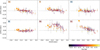 |
Fig. 7 Dependence of [X/Fe] on [Fe/H]. OCCASO+ data (Carbajo-Hijarrubia et al. 2024) are represented by triangles. Auner 1 and Berkeley 102 are shown as squares. All objects are colour-coded by age. |
5.2 Radial trends
In Fig. 8, we place Auner 1 and Berkeley 102 in the diagram of [Fe/H] versus galactocentric radius, together with the clusters of OCCASO+. We performed a linear fit to quantify the radial gradient. This fit was performed with the same method as in Anders et al. (2017), using a maximum likelihood algorithm as first guess, and computing a Markov chain Monte Carlo (MCMC) with the Python package emcee (Foreman-Mackey et al. 2013). The grey lines in the figure show the fits we made with MCMC, and the black line shows the best fit. The computed slope inside the knee radius is −0.068 ± 0.007 dex kpc−1, and outside the knee radius, it is −0.025 ± 0.011 dex kpc−1. The knee is at 11.4 ± 0.8 kpc. The fit agrees with the fit obtained by Carbajo-Hijarrubia et al. (2024); Myers et al. (2022); Magrini et al. (2022). The metallicities of Auner 1 and Berkeley 102 are slightly below the general trend, but they are compatible with the metallicities of other clusters at similar galactocentric radii. The four outermost clusters (Berkeley 21, Berkeley 31, Tombaugh 2, and Berkeley 29) are highly relevant to this fit because without them, we continue to find the knee, although the second slope is compatible with the first slope when the uncertainty is taken into account. The abundances we observe for Auner 1 and Berkeley 102 denote that the knee may be farther away from what we found when we evaluated the clusters we studied in the sample we presented, and the flattening may only occur in clusters beyond 14 kpc.
When we examine the radial trends of other elements with respect to iron (Fig. 9), the trends were analysed using MCMC, as outlined in the previous paragraph. The algorithm we employed determined whether a single slope or a combination of two slopes provided a better fit. The analysis shows that all elements are best described by a single slope, except for Ba, which is better described by two slopes. The α elements [Ca/Fe] and [Ti/Fe] show a mildly positive gradient, which agrees with the models of the inside-out formation of the Galactic disc. The Fe-peak elements [Co/Fe] and [Ni/Fe] show no radial gradients because they are produced by the same processes as Fe. Inside the knee (RGal ≤ 11.4 kpc), [Ba/Fe] shows a positive trend that is reversed in the outer disc. This pattern is produced by the dependence of the s-process production on [Fe/H], as discussed above. The [Eu/Fe] has a steep slope, which is consistent with its production mainly by r-process. The abundances of the two clusters are also compatible in general with those of the other clusters with similar galactocentric radii. In concordance with Fig. 7, the [Ca/Fe], [Ti/Fe], and [Eu/Fe] values for our clusters are slightly higher than the general trend, but still compatible within the 1σ uncertainties. As mentioned above, the [Eu/Fe] abundance in the cluster Berkeley 102 is similar to that of Berkeley 29, which is located at a larger galactocentric radius. We again remark the large intrinsic uncertainties in our measurements for this element. The abundances for the other elements of the two clusters coincide perfectly with those found in the OCCASO+ sample (Carbajo-Hijarrubia et al. 2024).
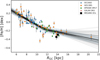 |
Fig. 8 Dependence of [Fe/H] on the galactocentric radius. The different sub-samples of OCCASO+ as in Fig. 14 Carbajo-Hijarrubia et al. (2024) are colour-coded. Auner 1 and Berkeley 102 are shown as black squares. The grey lines show the fits we made using MCMC, and the black line shows the best fit. |
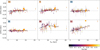 |
Fig. 9 Dependence of [X/Fe] on galactocentric radius. OCCASO+ data (Carbajo-Hijarrubia et al. 2024) are represented by triangles. Auner 1 and Berkeley 102 are shown as squares. All the objects are colour-coded by age. The black lines show the MCMC best fits to the OCCASO+ sample as derived by Carbajo-Hijarrubia et al. (2024). |
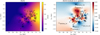 |
Fig. 10 Kriging maps of the metallicities of OCs in the Galactic plane. Left: [Fe/H] abundances. Right: residuals without the radial gradient (Fig. 8). The panels show the OCCASO+ sample (Carbajo-Hijarrubia et al. 2024). The Sun is situated at (−8.2, 0.0) in both maps. The MEGARA clusters Auner 1 and Berkeley 102 are shown as squares, and some other distant clusters included in OCCASO+ are also labelled. |
5.3 Azimuthal dependence
Figure 10 shows the Kriging maps3 of the metallicities of OCs observed by high-resolution spectroscopy in the Galactic plane. In particular, the right panel shows the Kriging map of the residuals without the radial gradient. Both panels show the clusters of the OCCASO+ sample (Carbajo-Hijarrubia et al. 2024), and the two clusters in this paper are shown as squares. The map of the [Fe/H] residuals shown in the right panel of Fig. 10 shows a certain structure that is not produced by the metallicity gradient. The pattern is similar to that reported by Poggio et al. (2022) in the regions in which our study and theirs overlap (i.e., within 4 kpc from the Sun). The authors explained this variation as produced by the formation of the stars in the region of the spiral arms or in the inter-arm region. We agree with Poggio et al. (2022) in the explanation. This dependence partially causes the dispersion of [Fe/H] for the same RGC. These maps feature well-sampled regions, primarily within a 3 kpc radius of the Sun. Some areas are dominated by a single cluster, however. These maps are therefore best suited for guiding our interpretation and planning future observing campaigns. Clearly, more observations of distant (in galactocentric distance and azimuth) open clusters with medium- to high-resolution instruments are needed to firmly establish the abundance trends of the outermost parts of the Galactic disc. Since our statistics are small, it is important to compare the relatively sparse open cluster sample with other abundance tracers that are visible at these distances, such as Cepheids or red giant stars.
5.4 Implications for the formation of outer-disc OCs
Galactic chemical evolution models based on the inside-out formation scenario often predict a continuously decreasing radial gradient (e.g. Prantzos et al. 2018; Kobayashi et al. 2020). The observed flattening can be matched when additional preenriched infall of material in the outer disc in Galactic chemical evolution models is included (Magrini et al. 2009). Similar patterns in metallicity are found in extragalactic studies based on ionised gas abundances (Bresolin et al. 2009, 2012). Resonances of bar or spiral arms (Lépine et al. 2011) or accretion of gas from the intergalactic medium have been proposed as mechanisms to explain this feature (Bresolin et al. 2012; Bowen et al. 2020). In a third scenario, the outer-disc OCs are associated with merger events, either acquired from merging galaxies Friel (2013) or formed as a result of the merger event itself (Yong et al. 2012; Magrini et al. 2009). Since the enrichment process in this zone would be different, a peculiar signature of abundances beyond metallicity is expected, but not observed (Carraro et al. 2007; Sestito et al. 2008). The OC orbits might also be affected by the trajectory of the merger galaxy and the reaction of the disc. Another possible scenario is that these clusters have formed in a more internal region of the disc and migrated outwards, producing the flat abundance gradients. This process was simulated (Roškar et al. 2008) and was proposed to explain the observed age-[Fe/H] distribution of outer-disc field stars (Lian et al. 2022). In this case, the chemical abundances of the outer-disc OCs should be those of the innermost regions at the time of its birth. Based on our analysis of the age, orbital parameters, and chemical abundances, we conclude that Auner 1 and Berkeley 102 are part of the thin-disc population. This evidence strongly challenges the hypothesis that the outermost open clusters originated in another galaxy and were later accreted during a merger event. The flattening pattern found in Fe in the outermost part of the disc is dominated by four open clusters that were observed by GES. Further research is needed in this region.
6 Summary and conclusions
We have used medium-resolution spectra (R ~ 18 700) obtained with the MEGARA instrument at the GTC to study red giant star members of the old and distant outer-disc clusters Auner 1 and Berkeley 102. These clusters have been studied spectroscopically for the first time, and to our knowledge, open clusters at these Galactic azimuths and radii have been observed for the first time as well. Only a few clusters were studied spectroscopically at the distance at which these OCs are located because this is beyond the capabilities of most telescopes and instruments because these stars are very faint (G ≥ 16). We determined radial velocities and atmospheric parameters for the member stars, and we updated the ages and distances for the two clusters. Finally, we measured the chemical abundances of seven chemical elements (Fe, Ca, Ti, Co, Ni, Ba, and Eu) using spectral synthesis, and we differentially corrected for abundance offsets with respect to high-resolution spectroscopy.
Our main findings are summarised below.
The radial velocities of the clusters and their orbits confirm that the kinematics of the two OCs are typical of the outer Galactic disc.
The [Fe/H] values of Auner 1 and Berkeley 102 follow the trend of other outer-disc clusters located at similar galac-tocentric radii, with indications of systematic azimuthal abundance variations, as also found in field-star studies.
The [Fe/H] abundances of Auner 1 and Berkeley 102 suggest that the knee position of the radial gradient may be sightly farther away than recent estimates (e.g., 11.2 kpc; Carbajo-Hijarrubia et al. 2024).
The [X/Fe] abundances follow the expected trends for the galactocentric distances of Auner 1 and Berkeley 102, and they are compatible with the OCCASO+ sample. Slightly higher values are found for [Ca/Fe] and [Eu/Fe], but they are still compatible within 1σ.
From the results of our analysis of the age, orbit, and chemical abundance, we conclude that Auner 1 and Berkeley 102 belong to the thin-disc population. From Gaia Collaboration (2021a), based on Gaia EDR3 data (Gaia Collaboration 2021b), we know that the two outermost known OCs of the Milky Way, Saurer 1 and Berkeley 29, are also very likely thin-disc objects. These facts combined provide strong evidence against the scenario that the outermost OCs formed in another galaxy and were captured during a merger event. The data obtained so far prevent us from distinguishing between the different outer-disc chemical evolution and migration scenarios proposed in the literature. In order to better characterize the knee position and to distinguish between these scenarios, it is essential to study more clusters in the outer disc. The capabilities of MEGARA at GTC make this possible and open a window into a largely unexplored area of the Milky Way.
Acknowledgements
This publication is based on data obtained with the MEGARA instrument at the Gran Telescopio Canarias, funded by European Regional Development Funds (ERDF) through Programa Operativo Canarias FEDER 2014-2020, and installed in the Spanish Observatorio del Roque de los Muchachos of the Instituto de Astrofísica de Canarias, on the island of La Palma. MEGARA has been built by a Consortium led by the Universidad Complutense de Madrid (Spain) and that also includes the Instituto de Astrofísica, Óptica y Electrónica (Mexico), Instituto de Astrofísica de Andalucía (CSIC, Spain) and the Univesidad Politécnica de Madrid (Spain). MEGARA is funded by the Consortium institutions and by GRANTECAN S.A. Based on observations made with the Gran Telescopio Canarias (GTC), installed at the Spanish Observatorio del Roque de los Muchachos of the Instituto de Astrofísica de Canarias, on the island of La Palma. This work is partly based on data from the GTC Public Archive at CAB (INTA-CSIC), developed in the framework of the Spanish Virtual Observatory project supported by the Spanish MINECO through grants AYA 2011-24052 and AYA 2014-55216. The system is maintained by the Data Archive Unit of the CAB (INTA-CSIC) This work has made use of data from the European Space Agency (ESA) mission Gaia (http://www.cosmos.esa.int/gaia), processed by the Gaia Data Processing and Analysis Consortium (DPAC, http://www.cosmos.esa.int/web/gaia/dpac/consortium). We acknowledge the Gaia Project Scientist Support Team and the Gaia DPAC. Funding for the DPAC has been provided by national institutions, in particular, the institutions participating in the Gaia Multilateral Agreement. This work was supported by the MINECO (Spanish Ministry of Economy, Industry and Competitiveness) through grant ESP2016-80079-C2-1-R (MINECO/FEDER, UE) and by the Spanish MICIN/AEI/10.13039/501100011033 and by “ERDF A way of making Europe” by the “European Union” through grants RTI2018-095076-B-C21 and PID2021-122842OB-C21, and the Institute of Cosmos Sciences University of Barcelona (ICCUB, Unidad de Excelencia “María de Maeztu”) through grant CEX2019-000918-M. FA and LC acknowledge the grants RYC2021-031683-I and RYC2021-033762-I, funded by MCIN/AEI/10.13039/501100011033 and by the European Union NextGenerationEU/PRTR. AGdP acknowledges financial support from the Spanish MICIN under grants PID2022-138621NB-I00 and PID2021-123417OB-I00. This research has made use of NASA’s Astrophysics Data System Bibliographic Services.
Appendix A Complementary tables and figures
This appendix contains three complementary tables: Table A.1 shows the results of our abundance analysis of a MEGARA spectrum of the Sun, Table A.2 shows the linelist used in our analysis of the MEGARA HR-R spectra, and Table A.3 lists the orbital parameters of the two clusters obtained under different assumptions.
Figures A.1 through A.6 show zoom-in plots into the spectra of the six red-giant stars in Auner 1 and Berkeley 102 used for abundance analysis. Figure A.7 shows the results of our differential analysis of APOGEE and MEGASTAR spectra.
Solar abundances obtained in this paper from our MEGARA spectra, compared with Grevesse et al. (2007, GAS07) and Asplund et al. (2009, AGS09).
List of lines for red giants observed with the HR-R grating.
Orbital parameters of the two clusters obtained with different Galactic potentials.
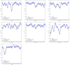 |
Fig. A.1 Spectrum of Auner_1_1 and spectral synthesis fit. |
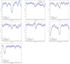 |
Fig. A.2 Spectrum of Auner_1_2 and spectral synthesis fit. |
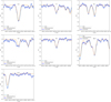 |
Fig. A.3 Spectrum of Auner_1_3 and spectral synthesis fit. |
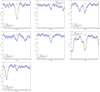 |
Fig. A.4 Spectrum of Berkeley_102_1 and spectral synthesis fit. |
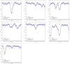 |
Fig. A.5 Spectrum of Berkeley_102_2 and spectral synthesis fit. |
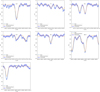 |
Fig. A.6 Spectrum of Berkeley_102_3 and spectral synthesis fit. |
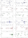 |
Fig. A.7 Difference between the chemical abundances obtained from MEGASTAR and APOGEE spectra, with respect to Teff, log g and abundance (in the sense APOGEE-MEGASTAR). Top left panels: [Fe/H]. Top right panels: [Ca/Fe]. Bottom left panels: [Co/Fe]. Bottom right panels: [Ni/Fe]. |
References
- Anders, F., Chiappini, C., Minchev, I., et al. 2017, A&A, 600, A70 [NASA ADS] [CrossRef] [EDP Sciences] [Google Scholar]
- Anders, F., Castro-Ginard, A., Casado, J., Jordi, C., & Balaguer-Núñez, L. 2022a, RNAAS, 6, 58 [Google Scholar]
- Anders, F., Khalatyan, A., Queiroz, A. B. A., et al. 2022b, A&A, 658, A91 [NASA ADS] [CrossRef] [EDP Sciences] [Google Scholar]
- Antoja, T., Figueras, F., Romero-Gómez, M., et al. 2011, MNRAS, 418, 1423 [NASA ADS] [CrossRef] [Google Scholar]
- Arellano-Córdova, K. Z., Esteban, C., García-Rojas, J., & Méndez-Delgado, J. E. 2020, MNRAS, 496, 1051 [Google Scholar]
- Asplund, M., Grevesse, N., Sauval, A. J., & Scott, P. 2009, ARA&A, 47, 481 [NASA ADS] [CrossRef] [Google Scholar]
- Balser, D. S., Rood, R. T., Bania, T. M., & Anderson, L. D. 2011, ApJ, 738, 27 [NASA ADS] [CrossRef] [Google Scholar]
- Blanco-Cuaresma, S. 2019, MNRAS, 486, 2075 [Google Scholar]
- Blanco-Cuaresma, S., Soubiran, C., Heiter, U., & Jofré, P. 2014, A&A, 569, A111 [CrossRef] [EDP Sciences] [Google Scholar]
- Boeche, C., Siebert, A., Piffl, T., et al. 2014, A&A, 568, A71 [NASA ADS] [CrossRef] [EDP Sciences] [Google Scholar]
- Bovy, J. 2015, ApJS, 216, 29 [NASA ADS] [CrossRef] [Google Scholar]
- Bovy, J., Leung, H. W., Hunt, J. A. S., et al. 2019, MNRAS, 490, 4740 [Google Scholar]
- Bowen, D. V., Tripp, T. M., Jenkins, E. B., et al. 2020, ApJ, 893, 84 [Google Scholar]
- Bragança, G. A., Daflon, S., Lanz, T., et al. 2019, A&A, 625, A120 [NASA ADS] [CrossRef] [EDP Sciences] [Google Scholar]
- Bresolin, F., Ryan-Weber, E., Kennicutt, R. C., & Goddard, Q. 2009, ApJ, 695, 580 [Google Scholar]
- Bresolin, F., Kennicutt, R. C., & Ryan-Weber, E. 2012, ApJ, 750, 122 [NASA ADS] [CrossRef] [Google Scholar]
- Cantat-Gaudin, T., Anders, F., Castro-Ginard, A., et al. 2020, A&A, 640, A1 [NASA ADS] [CrossRef] [EDP Sciences] [Google Scholar]
- Carbajo-Hijarrubia, J., Casamiquela, L., Carrera, R., et al. 2024, A&A, 687, A239 [NASA ADS] [CrossRef] [EDP Sciences] [Google Scholar]
- Carraro, G., Geisler, D., Villanova, S., Frinchaboy, P. M., & Majewski, S. R. 2007, A&A, 476, 217 [NASA ADS] [CrossRef] [EDP Sciences] [Google Scholar]
- Carrasco, E., Gil de Paz, A., Gallego, J., et al. 2018, SPIE Conf. Ser., 10702, 1070216 [NASA ADS] [Google Scholar]
- Carrera, R., & Pancino, E. 2011, A&A, 535, A30 [NASA ADS] [CrossRef] [EDP Sciences] [Google Scholar]
- Carrera, R., Casamiquela, L., Carbajo-Hijarrubia, J., et al. 2022, A&A, 658, A14 [NASA ADS] [CrossRef] [EDP Sciences] [Google Scholar]
- Casamiquela, L., Tarricq, Y., Soubiran, C., et al. 2020, A&A, 635, A8 [NASA ADS] [CrossRef] [EDP Sciences] [Google Scholar]
- Chambers, K. C., Magnier, E. A., Metcalfe, N., et al. 2016, arXiv e-prints, [arXiv:1612.05560] [Google Scholar]
- Cox, D. P., & Gómez, G. C. 2002, ApJS, 142, 261 [NASA ADS] [CrossRef] [Google Scholar]
- Cristallo, S., Straniero, O., Gallino, R., et al. 2009, ApJ, 696, 797 [NASA ADS] [CrossRef] [Google Scholar]
- Cutri, R. M., Skrutskie, M. F., van Dyk, S., et al. 2003, VizieR Online Data Catalog: 2MASS All-Sky Catalog of Point Sources (Cutri+ 2003), VizieR On-line Data Catalog: II/246. Originally published in: University of Massachusetts and Infrared Processing and Analysis Center (IPAC/California Institute of Technology) [Google Scholar]
- Cutri, R. M., Wright, E. L., Conrow, T., et al. 2013, Explanatory Supplement to the AllWISE Data Release Products, Explanatory Supplement to the AllWISE Data Release Products, by R. M. Cutri et al. [Google Scholar]
- da Silva, R., Crestani, J., Bono, G., et al. 2022, A&A, 661, A104 [NASA ADS] [CrossRef] [EDP Sciences] [Google Scholar]
- da Silva, R., D’Orazi, V., Palla, M., et al. 2023, A&A, 678, A195 [NASA ADS] [CrossRef] [EDP Sciences] [Google Scholar]
- Daflon, S., & Cunha, K. 2004, ApJ, 617, 1115 [NASA ADS] [CrossRef] [Google Scholar]
- Ferrers, N. 1877, Q. J. Pure Appl. Math., 14, 1 [Google Scholar]
- Foreman-Mackey, D., Conley, A., Meierjurgen Farr, W., et al. 2013, emcee: The MCMC Hammer, Astrophysics Source Code Library [record asci:1303.002] [Google Scholar]
- Freiburghaus, C., Rosswog, S., & Thielemann, F. K. 1999, ApJ, 525, L121 [NASA ADS] [CrossRef] [Google Scholar]
- Friel, E. D. 2013, in Planets, Stars and Stellar Systems, 5: Galactic Structure and Stellar Populations, eds. T. D. Oswalt, & G. Gilmore, 347 [Google Scholar]
- Gaia Collaboration (Antoja, T., et al.) 2021a, A&A, 649, A8 [EDP Sciences] [Google Scholar]
- Gaia Collaboration (Brown, A. G. A., et al.) 2021b, A&A, 649, A1 [NASA ADS] [CrossRef] [EDP Sciences] [Google Scholar]
- Gallino, R., Arlandini, C., Busso, M., et al. 1998, ApJ, 497, 388 [Google Scholar]
- Gallino, R., Bisterzo, S., Straniero, O., Ivans, I. I., & Käppeler, F. 2006, Mem. Soc. Astron. Italiana, 77, 786 [Google Scholar]
- Genovali, K., Lemasle, B., Bono, G., et al. 2014, A&A, 566, A37 [NASA ADS] [CrossRef] [EDP Sciences] [Google Scholar]
- Gil de Paz, A., Carrasco, E., Gallego, J., et al. 2018, SPIE Conf. Ser., 10702, 1070217 [NASA ADS] [Google Scholar]
- Gómez-Álvarez, P., Castillo, A., Iglesias-Páramo, J., et al. 2018, SPIE Conf. Ser., 10707, 107071L [Google Scholar]
- Grevesse, N., Asplund, M., & Sauval, A. J. 2007, Space Sci. Rev., 130, 105 [Google Scholar]
- Hanuschik, R. W. 2003, A&A, 407, 1157 [NASA ADS] [CrossRef] [EDP Sciences] [Google Scholar]
- Heiter, U., Lind, K., Bergemann, M., et al. 2021, A&A, 645, A106 [EDP Sciences] [Google Scholar]
- Hunt, E. L., & Reffert, S. 2024, A&A, 686, A42 [NASA ADS] [CrossRef] [EDP Sciences] [Google Scholar]
- Jasniewicz, G., & Mayor, M. 1988, A&A, 203, 329 [NASA ADS] [Google Scholar]
- Kajino, T., Aoki, W., Balantekin, A. B., et al. 2019, Progr. Particle Nuclear Phys., 107, 109 [Google Scholar]
- Karakas, A. I., & Lattanzio, J. C. 2014, PASA, 31, e030 [NASA ADS] [CrossRef] [Google Scholar]
- Kobayashi, C., Karakas, A. I., & Lugaro, M. 2020, ApJ, 900, 179 [Google Scholar]
- Lépine, J. R. D., Cruz, P., Scarano, S., J., et al. 2011, MNRAS, 417, 698 [CrossRef] [Google Scholar]
- Lian, J., Zasowski, G., Hasselquist, S., et al. 2022, MNRAS, 511, 5639 [NASA ADS] [CrossRef] [Google Scholar]
- Lindegren, L., Bastian, U., Biermann, M., et al. 2021, A&A, 649, A4 [EDP Sciences] [Google Scholar]
- Luck, R. E. 2018, AJ, 156, 171 [Google Scholar]
- Maciel, W. J., Quireza, C., & Costa, R. D. D. 2007, A&A, 463, L13 [NASA ADS] [CrossRef] [EDP Sciences] [Google Scholar]
- Magrini, L., Sestito, P., Randich, S., & Galli, D. 2009, A&A, 494, 95 [NASA ADS] [CrossRef] [EDP Sciences] [Google Scholar]
- Magrini, L., Vázquez, C. V., Casali, G., et al. 2022, Universe, 8, 64 [NASA ADS] [CrossRef] [Google Scholar]
- Méndez-Delgado, J. E., Amayo, A., Arellano-Córdova, K. Z., et al. 2022, MNRAS, 510, 4436 [CrossRef] [Google Scholar]
- Minniti, J. H., Sbordone, L., Rojas-Arriagada, A., et al. 2020, A&A, 640, A92 [EDP Sciences] [Google Scholar]
- Mollá, M., García-Vargas, M. L., Millán-Irigoyen, I., et al. 2023, MNRAS, 519, 5472 [Google Scholar]
- Myers, N., Donor, J., Spoo, T., et al. 2022, AJ, 164, 85 [NASA ADS] [CrossRef] [Google Scholar]
- Navarro, J. F., Frenk, C. S., & White, S. D. M. 1997, ApJ, 490, 493 [Google Scholar]
- Nguyen, C. T., Costa, G., Girardi, L., et al. 2022, A&A, 665, A126 [NASA ADS] [CrossRef] [EDP Sciences] [Google Scholar]
- Nishimura, S., Kotake, K., Hashimoto, M.-a., et al. 2006, ApJ, 642, 410 [NASA ADS] [CrossRef] [Google Scholar]
- Onken, C. A., Wolf, C., Bessell, M. S., et al. 2019, PASA, 36, e033 [Google Scholar]
- Pascual, S., Cardiel, N., Castillo-Morales, Á., Picazo-Sánchez, P., & Gil de Paz, A. 2024, https://doi.org/10.5281/zenodo.14193498 [Google Scholar]
- Perren, G. I., Pera, M. S., Navone, H. D., & Vázquez, R. A. 2022, A&A, 663, A131 [NASA ADS] [CrossRef] [EDP Sciences] [Google Scholar]
- Poggio, E., Recio-Blanco, A., Palicio, P. A., et al. 2022, A&A, 666, L4 [NASA ADS] [CrossRef] [EDP Sciences] [Google Scholar]
- Prantzos, N., Abia, C., Limongi, M., Chieffi, A., & Cristallo, S. 2018, MNRAS, 476, 3432 [Google Scholar]
- Reid, M. J., Menten, K. M., Brunthaler, A., et al. 2014, ApJ, 783, 130 [Google Scholar]
- Reid, M. J., Menten, K. M., Brunthaler, A., et al. 2019, ApJ, 885, 131 [Google Scholar]
- Roesslein, M., Wolf, M., Wampfler, B., & Wegscheider, W. 2007, Springer, 12, 495 [Google Scholar]
- Romero-Gómez, M., Athanassoula, E., Antoja, T., & Figueras, F. 2011, MNRAS, 418, 1176 [CrossRef] [Google Scholar]
- Romero-Gómez, M., Figueras, F., Antoja, T., Abedi, H., & Aguilar, L. 2015, MNRAS, 447, 218 [CrossRef] [Google Scholar]
- Roškar, R., Debattista, V. P., Quinn, T. R., Stinson, G. S., & Wadsley, J. 2008, ApJ, 684, L79 [Google Scholar]
- Schönrich, R., Binney, J., & Dehnen, W. 2010, MNRAS, 403, 1829 [NASA ADS] [CrossRef] [Google Scholar]
- Sestito, P., Bragaglia, A., Randich, S., et al. 2008, A&A, 488, 943 [NASA ADS] [CrossRef] [EDP Sciences] [Google Scholar]
- Soubiran, C., Cantat-Gaudin, T., Romero-Gómez, M., et al. 2018, A&A, 619, A155 [NASA ADS] [CrossRef] [EDP Sciences] [Google Scholar]
- Spina, L., Ting, Y. S., De Silva, G. M., et al. 2021, MNRAS, 503, 3279 [CrossRef] [Google Scholar]
- Stanghellini, L., & Haywood, M. 2018, ApJ, 862, 45 [Google Scholar]
- Surman, R., McLaughlin, G. C., Ruffert, M., Janka, H. T., & Hix, W. R. 2008, ApJ, 679, L117 [NASA ADS] [CrossRef] [Google Scholar]
- Thygesen, A. O., Frandsen, S., Bruntt, H., et al. 2012, A&A, 543, A160 [NASA ADS] [CrossRef] [EDP Sciences] [Google Scholar]
- Watson, D., Hansen, C. J., Selsing, J., et al. 2019, Nature, 574, 497 [NASA ADS] [CrossRef] [Google Scholar]
- Woosley, S. E., Wilson, J. R., Mathews, G. J., Hoffman, R. D., & Meyer, B. S. 1994, ApJ, 433, 229 [Google Scholar]
- Yong, D., Carney, B. W., & Friel, E. D. 2012, AJ, 144, 95 [Google Scholar]
When the observations were planned, the catalogue of (Hunt & Reffert 2024) was not yet available.
All Tables
Solar abundances obtained in this paper from our MEGARA spectra, compared with Grevesse et al. (2007, GAS07) and Asplund et al. (2009, AGS09).
Orbital parameters of the two clusters obtained with different Galactic potentials.
All Figures
|
Fig. 1 Spatial distribution in the field of the IFU. We mark the stars that were observed inside the field of view of MEGARA with squares. |
| In the text | |
|
Fig. 2 Sky positions, proper motions, parallax vs. magnitude, and CMD of Auner 1 (top panels) and Berkeley 102 (bottom panels). We show all the stars in the region (black points) and the stars that were considered members of each cluster by Cantat-Gaudin et al. (2020) (red circles) and Hunt & Reffert (2024) (blue circles). We mark the observed stars with orange squares. |
| In the text | |
|
Fig. 3 Colour-magnitude diagram of Auner 1 (right) and Berkeley 102 (left). Stars in the field are marked as grey dots, and those that were considered members by Cantat-Gaudin et al. (2020) are shown as red circles and those by Hunt & Reffert (2024) as blue circles. We also mark the observed stars with orange squares (those in Berkeley 102 overlap). We superimpose the isochrone fitting of Cantat-Gaudin et al. (2020) (red), Hunt & Reffert (2024) (blue), and ours (black). |
| In the text | |
|
Fig. 4 Projection onto the Galactic plane of the position and velocity with respect to the RSR of our two clusters (squares) and Carrera et al. (2022) (circles), coloured by age. We also depict the spiral arms determined by Reid et al. (2019). |
| In the text | |
|
Fig. 5 Orbits of Auner 1 (left) and Berkeley 102 (right) for potentials MW2014 (blue), MW2014 + arms (green), and MW2014 + bar (yellow). |
| In the text | |
|
Fig. 6 Dependence of the orbital parameters zmax (top) and eccentricity (bottom) on the age and galactocentric radius of OCs. In the top panel, we fit the data with an exponential function. Objects observed with MEGARA are marked with circles, and objects observed with OCCASO (Carrera et al. 2022) are shown as triangles. In all of them, the galactocentric radius is colour-coded. |
| In the text | |
|
Fig. 7 Dependence of [X/Fe] on [Fe/H]. OCCASO+ data (Carbajo-Hijarrubia et al. 2024) are represented by triangles. Auner 1 and Berkeley 102 are shown as squares. All objects are colour-coded by age. |
| In the text | |
|
Fig. 8 Dependence of [Fe/H] on the galactocentric radius. The different sub-samples of OCCASO+ as in Fig. 14 Carbajo-Hijarrubia et al. (2024) are colour-coded. Auner 1 and Berkeley 102 are shown as black squares. The grey lines show the fits we made using MCMC, and the black line shows the best fit. |
| In the text | |
|
Fig. 9 Dependence of [X/Fe] on galactocentric radius. OCCASO+ data (Carbajo-Hijarrubia et al. 2024) are represented by triangles. Auner 1 and Berkeley 102 are shown as squares. All the objects are colour-coded by age. The black lines show the MCMC best fits to the OCCASO+ sample as derived by Carbajo-Hijarrubia et al. (2024). |
| In the text | |
|
Fig. 10 Kriging maps of the metallicities of OCs in the Galactic plane. Left: [Fe/H] abundances. Right: residuals without the radial gradient (Fig. 8). The panels show the OCCASO+ sample (Carbajo-Hijarrubia et al. 2024). The Sun is situated at (−8.2, 0.0) in both maps. The MEGARA clusters Auner 1 and Berkeley 102 are shown as squares, and some other distant clusters included in OCCASO+ are also labelled. |
| In the text | |
|
Fig. A.1 Spectrum of Auner_1_1 and spectral synthesis fit. |
| In the text | |
|
Fig. A.2 Spectrum of Auner_1_2 and spectral synthesis fit. |
| In the text | |
|
Fig. A.3 Spectrum of Auner_1_3 and spectral synthesis fit. |
| In the text | |
|
Fig. A.4 Spectrum of Berkeley_102_1 and spectral synthesis fit. |
| In the text | |
|
Fig. A.5 Spectrum of Berkeley_102_2 and spectral synthesis fit. |
| In the text | |
|
Fig. A.6 Spectrum of Berkeley_102_3 and spectral synthesis fit. |
| In the text | |
|
Fig. A.7 Difference between the chemical abundances obtained from MEGASTAR and APOGEE spectra, with respect to Teff, log g and abundance (in the sense APOGEE-MEGASTAR). Top left panels: [Fe/H]. Top right panels: [Ca/Fe]. Bottom left panels: [Co/Fe]. Bottom right panels: [Ni/Fe]. |
| In the text | |
Current usage metrics show cumulative count of Article Views (full-text article views including HTML views, PDF and ePub downloads, according to the available data) and Abstracts Views on Vision4Press platform.
Data correspond to usage on the plateform after 2015. The current usage metrics is available 48-96 hours after online publication and is updated daily on week days.
Initial download of the metrics may take a while.