| Issue |
A&A
Volume 589, May 2016
|
|
|---|---|---|
| Article Number | A104 | |
| Number of page(s) | 12 | |
| Section | The Sun | |
| DOI | https://doi.org/10.1051/0004-6361/201527249 | |
| Published online | 20 April 2016 | |
Plasma motions and non-thermal line broadening in flaring twisted coronal loops
1
Jodrell Bank Centre for Astrophysics, University of
Manchester,
Manchester
M13 9PL,
UK
e-mail:
This email address is being protected from spambots. You need JavaScript enabled to view it.
2
Astronomy & Astrophysics Group, University of
Glasgow, Glasgow
G15 8QQ,
UK
Received: 25 August 2015
Accepted: 27 January 2016
Abstract
Context. Observation of coronal extreme ultra-violet (EUV) spectral lines sensitive to different temperatures offers an opportunity to evaluate the thermal structure and flows in flaring atmospheres. This, in turn, can be used to estimate the partitioning between the thermal and kinetic energies released in flares.
Aims. Our aim is to forward-model large-scale (50–10 000 km) velocity distributions to interpret non-thermal broadening of different spectral EUV lines observed in flares. The developed models allow us to understand the origin of the observed spectral line shifts and broadening, and link these features to particular physical phenomena in flaring atmospheres.
Methods. We use ideal magnetohydrodynamics (MHD) to derive unstable twisted magnetic fluxtube configurations in a gravitationally stratified atmosphere. The evolution of these twisted fluxtubes is followed using resistive MHD with anomalous resistivity depending on the local density and temperature. The model also takes thermal conduction and radiative losses in the continuum into account. The model allows us to evaluate average velocities and velocity dispersions, which would be interpreted as non-thermal velocities in observations, at different temperatures for different parts of the models.
Results. Our models show qualitative and quantitative agreement with observations. Thus, the line-of-sight (LOS) velocity dispersions demonstrate substantial correlation with the temperature, increasing from about 20–30 km s-1 around 1 MK to about 200–400 km s-1 near 10–20 MK. The average LOS velocities also correlate with velocity dispersions, although they demonstrate a very strong scattering compared to the observations. We also note that near footpoints the velocity dispersions across the magnetic field are systematically lower than those along the field. We conclude that the correlation between the flow velocities, velocity dispersions, and temperatures are likely to indicate that the same heating mechanism is responsible for heating the plasma, its turbulisation, and expansion/evaporation.
Key words: Sun: flares / Sun: UV radiation / Sun: magnetic fields / magnetic reconnection / magnetohydrodynamics (MHD)
© ESO, 2016
1. Introduction
 |
Fig. 1 Evolution of Model L1. Left column: magnetic field lines; red and blue field lines are tied to opposite footpoints of the twisted loop; yellow lines denote ambient field. Middle column: temperature distribution; yellow patchy surface corresponds to 2 MK; orange and blue surfaces correspond to 3 and 4 MK, respectively. Right column: surfaces of j = jcrit, i.e. showing the locations with fast magnetic energy release. Times (after onset of the instability) are shown for each row on the left in units of characteristic Alfvén times tA, which are 0.44 s for this model. |
Plasma motions in the flaring solar corona are closely related to heating processes and can be used to study the spatial distribution of energy release and the dynamics of energy transfer. New instruments on board recent solar space missions, such as Hinode/EIS and SDO/AIA, offer an opportunity to study characteristics of very hot (~1–10 MK and hotter) plasma in a flaring atmosphere with high spatial resolution (Culhane et al. 2007; Lement et al. 2012). Observations show that solar flares have a complex plasma flow structure at different spatial scales (e.g. Watanabe et al. 2010; Del Zanna et al. 2011). Furthermore, flare kernels often reveal coronal lines with complex Doppler structure, containing both red-shifted and blue-shifted components (e.g. Young et al. 2013), indicating that plasma motions are inhomogeneous in spatially unresolved volumes.
Analysis of the Doppler shift structure in coronal lines shows that colder plasma (T ≈ 0.1–1 MK) normally moves downwards with velocities of about 20–50 km s-1, while the hotter plasma (T ≈ 1–10 MK) shows upflow; this upflowing plasma is very inhomogeneous, showing velocities from only few km s-1 up to 400–500 km s-1 (see Doschek et al. 2007, 2008, 2013; Del Zanna 2008; Watanabe et al. 2010; Young et al. 2013). It is also noted that the downflow plasma can be substantially denser (n ~ 3 × 10¹⁶ m-3) than the upflow plasma (n ~ 5 × 10¹⁴ − 1015 m-3), which is probably why the downflow is easier to observe than the upflow (e.g. Del Zanna 2008; Doschek et al. 2008).
Most coronal lines in flares also demonstrate non-thermal broadening due to additional velocity dispersion (e.g. Doschek et al. 2007). The non-thermal velocity appears to correlate with the bulk plasma velocity. For instance, in two flares analysed by Doschek et al. (2008) using Hinode data, non-thermal velocity dispersion is higher at locations with higher upflow speed; the velocity dispersion is about 25–30 km s-1 when the upflow speed is nearly zero, and is about 50–60 km s-1 when the upflow velocity is 20 km s-1. The non-thermal velocities, which appear early in solar flares (see e.g. Harra et al. 2013), have also been found to correlate with plasma temperature. The non-thermal velocities have the lowest values near 1 MK: from 0 to 20–40 km s-1. At lower temperatures (0.1–1 MK) these velocities are higher at about 40–60 km s-1. At the same time, at high temperatures (10–20 MK) they can be as much as 100–130 km s-1. The non-thermal velocities at high temperatures vary during the flare, and they peak very close to the hard X-ray maximum at about 100 km s-1 (some observers note much higher values, up to 380 km s-1; see e.g. Cirtain et al. 2013), and then during the decay phase of the flare reduce to about 50 km s-1 (Susino et al. 2013).
The bulk plasma flows are normally interpreted as a vertical advection of plasmas in stratified atmosphere due to heating in the chromosphere, transition region, or lower corona. As far as the non-thermal line broadening is concerned, there are several viable interpretations. Firstly, this can be due to the turbulence, which can occur in a very hot plasma in post-reconnection loops or directly at the primary energy release location. The latter is compatible with the idea that the reconnection should occur in a very turbulent medium, and this turbulence would facilitate the magnetic diffusion (see e.g. Lazarian & Vishniak 1999; Browning & Lazarian 2013). It is also expected that the plasma in flaring coronal loops is strongly turbulent owing to relatively fast heating (by energetic particles, waves, shocks, conduction, etc.). Secondly, coronal lines can also be broadened due to unresolved inhomogeneity of regular flows (either in the plane perpendicular to the line-of-sight – LOS, or along the LOS). This is possible, particularly, in the lower corona and the chromosphere, which can have small-scale structure (as small as ~100 km; see e.g. Antolin & Rouppe van der Voort 2012; Gordovskyy & Lozitsky 2014). The velocity field can also be highly non-uniform in a relatively small volume occupied by the exhaust from reconnecting current layer (e.g. Vrsnak et al. 2009; Ko et al. 2010).
The issue of plasma turbulence in solar flares is intimately connected to the problem of energy partitioning. There are several estimations of the energy partitioning in flares, but they appear to be very different, changing from flare to flare (see e.g. Emslie et al. 2004; Fleishman et al. 2015). The problem is that all observational estimations appear to depend strongly on the instrument properties (see e.g. Benz 2008). Furthermore, there is a substantial uncertainty about the total energy of non-thermal particles; this energy depends on the low-energy part of the spectra, which, in turn, depends on the so-called lower energy cut-off, which is still under discussion (e.g. Kontar et al. 2008). Diagnostics of thermal plasma can also be difficult, particularly of low-temperature plasma, which is less visible in extreme ultra-violet (EUV) continuum and contributes less to coronal spectral lines. Indeed, an adequate evaluation of the turbulent velocities is necessary to determine what part of the energy is released as either kinetic, thermal, magnetic, or potential energy. The first two types depend on the plasma flows, turbulence, temperature, and density distributions in the plasma and energetic (i.e. non-Maxwellian) particle spectra. In this study, we derive the parameters of thermal plasma from our magnetohydrodynamic (MHD) models.
Most studies interpret these observations based on the so-called standard model of solar flares. At the same time, flare models based on magnetic reconnection in kink-unstable twisted coronal loops (Browning et al. 2008; Hood et al. 2009; Gordovskyy & Browning 2012; Bareford et al. 2013; Gordovskyy et al. 2013, 2014), which are more relevant to confined flares within single loops, offer a good opportunity to investigate plasma motion in flaring loops at different spatial scales, that is, from ~100 km to ~10 Mm. One advantage of this scenario is that it offers both configurations with rather localised heating (at the loop-top and/or near footpoints) and configurations with heating sources uniformly distributed along flaring loops. Characteristics of plasma motion are defined predominantly by the distribution of plasma heating sources (due to Ohmic dissipation, high-energy particle thermalisation, etc.) and their temporal evolution, and by thermal conduction and radiative energy losses. Hence, even though the considered models are not a universal flare scenario, and do not account for energy transfer by energetic particles, the results obtained with these models can be extrapolated to a wide range of flare configurations and scenarios.
In the present paper, we study turbulent plasma motions, resulting in non-thermal broadening of spectral lines. Our models make it possible to investigate the velocity field with a spatial scale of ~100 km, which is the grid-step in the z-direction, and is not resolved in majority of observations. We derive characteristics, which are direct proxies for measured parameters, and discuss them in context of observational data.
2. Main features of the considered flare model
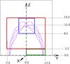 |
Fig. 2 Locations of sampling boxes in the domain: green box denotes the footpoint region, red box denotes the coronal region, and the blue box denotes the loop-top region. For models S1 and S2 the units are 1 Mm, while for larger models L1 and L2 the units are 4 Mm. |
We consider four different models of kink-unstable coronal loops with parameters typical for a flaring atmosphere:
-
Model S1 has a loop lengths of about 20 Mm with the apex at about 10 Mm. Its footpoint magnetic field is 95 G. Field geometry of this loop is very similar to those described by Gordovskyy et al. (2014) and Pinto et al. (2016). The model box has dimensions x = [ − 10; + 10 ] Mm, y = [ − 10; + 10 ] Mm, and z = [ 0; + 20 ] Mm. The axes are shown in Fig. 2.
-
Model S2 is considered in the same numerical box and has the same parameters as model S1, apart from a stronger footpoint magnetic field, which is 200 G.
-
Model L1 has similar configuration to smaller loops (S1 and S2) but is proportionally larger and has stronger field. Its length is about 80 Mm and footpoint strength is 700 G. The numerical box is x = [ − 40; + 40 ] Mm, y = [ − 40; + 40 ] Mm, and x = [ 0; + 80 ] Mm.
-
Model L2 is considered in the same numerical box and has the same parameters asmodel L1, apart from stronger footpoint magnetic field, which is 1500 G.
It is assumed that the lower boundary corresponds to the same level in the solar atmosphere in all the four models and, hence, the lower boundary has the same density in all models, 1020 m-3 (approximately corresponding to the upper chromosphere).
The loops are all embedded into gravitationally stratified atmosphere. The initial density in the atmosphere is  (1)where the density constants are ρ1 = 3.34 × 10⁻⁵ kg m-3 and ρ2 = 2 × 10-12 kg m-3, and the density length scales are zsc 1 = 0.25 Mm and zsc 2 = 50 Mm. The shift zsh = 1.5 Mm, putting the lower boundary of the computational domain approximately at the height of the lower chromosphere. The initial density at the upper boundary is 1015 m-3 in themodels S1 andS2, and 3 × 10¹⁴ m-3 in L1 and L2. The gravity acceleration is assumed to be constant g = 275 m s-2, so that the initial pressure can be easily obtained from density, as dpt = 0(z)/dz = − ρt = 0(z)g. As the density constants ρ1 and ρ2, and the length scales zsc 1 and zsc 2 are very different, there are two regions with nearly constant temperatures: around 104 K below 2 Mm, and about 0.9 MK about 2 Mm (see Gordovskyy et al. 2014). The magnetic field is strongly convergent, i.e. it is about ten times weaker near the loop apex, compared to the footpoints. This means that the fluxtube cross-section radius near the apex is around 3.2 times larger than that near footpoints. The modelling has been performed using the LARE3D code by Arber et al. (2001). The simulations are based on the resistive single-fluid MHD, also incorporating Braginskii thermal conduction (Braginskii 1965) and radiative losses following Klimchuk et al. (2008).
Pre-kink configurations have been derived as described in Gordovskyy et al. (2013), Bareford et al. (2016), Pinto et al. (2016). Although the initial atmosphere is in the hydrodynamical equilibrium, it is not stationary because of the thermal conduction. The heat flux from the hot corona to colder chromosphere results in noticeable changes of the temperature around the transition region. Moderate heating of the transition region and chromosphere and moderate cooling of the lower corona lead to smoother temperature profiles near the transition region (see Pinto et al. 2016; Bareford et al. 2016). The atmosphere settles in about ~1000 tA and only after this the initially potential loop is twisted by footpoint rotation. The twisting is very slow, the maximum linear velocity in small models is about 10 (or ~3 km s-1), which is always lower than local Alfven and sound velocities. Hence, during the twisting phase loops undergo sequences of nearly force-free states until kink instability onset. As the result, the loop undergoes a sequence of nearly force-free states during the twisting. Also, the twisting velocity is well below the observed LOS velocities and velocity dispersions (≥10 km s-1).
The kink instability occurs when the total twist reaches 6π − 8π (see also Bareford et al. 2016, for details). The magnetic reconnection in twisted coronal loops atmosphere after kink instability has been described in many earlier studies (see Hood & Priest 1979; Baty & Heyvaerts 1996; Browning & Van der Linden 2003; Hood et al. 2009; Gordovskyy & Browning 2012; Gordovskyy et al. 2014; Bareford et al. 2016), while the evolution of thermal and non-thermal radiation from such systems is considered by Botha et al. (2012), Gordovskyy et al. (2013, 2014), Pinto et al. (2016). Essentially, a loop experiences two different types of reconnection simultaneously: the reconnection between field lines of twisted fluxtube, resulting in twist reduction, and the reconnection of twisted field lines with the ambient field, resulting in the radial expansion of twisted loops (Fig. 1). The plasma temperature and, hence, thermal emission intensities peak towards the end of fast reconnection, when the twist is considerably lower. As the result, the visible twist in EUV/SXR is much lower than the critical twist required for the kink instability (Pinto et al. 2016).
3. Unresolved plasma motions in different temperature ranges
3.1. Macroscopic velocity distributions and their relation with non-thermal line broadening
Here we derive expressions relating the resolved flow velocities and unresolved flow velocity distribution to widths and positions of spectral lines (see e.g. Hubeny & Mihalas 2014, for exact derivations).
Assume the model contains only fully ionised hydrogen plasma, so that the electron and proton particle densities and total numbers are equal, that is np = ne = n and Np = Ne = N respectively. Further, assume that within an unresolved volume has a distribution of plasma in respect to the LOS velocity v|| and temperature T,  . Then, the profile of a spectral line emitted by this volume of plasma is
  (2)where a(T) is a temperature contribution function for the spectral line, s(λ − λline) is the line profile in the absence of macroscopic plasma motion.
The function s is normally a Gaussian-like profile, which can be approximated by a Gaussian  (3)where the Doppler width is
  . In fact, the exact shape of the s function is not important, as far as it is a Gaussian-like distribution, i.e. a distribution, becoming 0 at ±∞ with finite dispersion.
Assuming that the function  is also Gaussian in respect to the LOS velocity, i.e.
 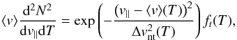 (4)the Eq. (2) can be written (using the convolution of two Gaussian functions) as
 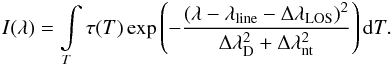 (5)Here
  represents so-called non-thermal contribution to line broadening, while
  , and τ(T) is the product of a(T), ft(T) and constants.
Hence, if the plasma’s distribution for each small temperature interval in the considered volume has some Gaussian-like distribution in respect to v||, then the average velocity, determining the line shift can be derived as follows: 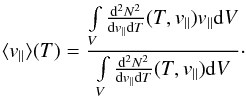 (6)(For this average LOS velocity we use the notation ⟨ v ⟩ hereafter.) The half-width of this distribution (or FWHM), which determines the non-thermal broadening of spectral line can be approximated as follows (this expression is exact for a Gaussian profile):
  (7)(For this LOS velocity dispersion (or variance) we use the notation Δvnt hereafter.)
In our simulation, we use discrete forms of Eqs. (6) and (7), i.e. ![Mathematical equation: \begin{eqnarray} \langle v \rangle_t &=& \frac {\sum \limits_\Omega [w_{ti} \; v_{||\,i} \; \delta\Omega]}{\sum \limits_\Omega [w_{ti} \; \delta\Omega]} \nonumber \\ \Delta v_{\it nt\;t}^2 &=& \frac {\sum \limits_\Omega [w_{ti} \; (v_{||\,i}-\langle v \rangle_t)^2 \; \delta\Omega]}{\sum \limits_\Omega [w_{ti} \; \delta\Omega]} \nonumber , \end{eqnarray}](/articles/aa/full_html/2016/05/aa27249-15/aa27249-15-eq63.png) where
where  In these equations, the index t corresponds to a temperature interval, index i corresponds to a grid points, and ΔΩ is an elementary volume between adjacent grid points (constant, as the grid is uniform in each direction). Here wti is, effectively, the density of plasma squared with temperature Tt and velocity v| | i, and, hence, corresponds to
  in Eqs. ((6), (7)). The integration goes over all the grid points in the considered volume Ω.
In the above equations, the integral ![Mathematical equation: \begin{eqnarray*} M_t=\sum \limits_\Omega [w_{ti} \; \delta\Omega] \end{eqnarray*}](/articles/aa/full_html/2016/05/aa27249-15/aa27249-15-eq73.png) is, in effect, the differential emission measure for the volume Ω. (In observations it is calculated as d [ n2(T)V(T) ] / dT or n2(dT/ dl)-1 for an individual pixel.)
is, in effect, the differential emission measure for the volume Ω. (In observations it is calculated as d [ n2(T)V(T) ] / dT or n2(dT/ dl)-1 for an individual pixel.)
In Sect. 3.2 the velocities ⟨ v ⟩ and Δvnt are calculated as functions of temperature using the above equations and compared with observational data.
 |
Fig. 3 Model S1. Left column: differential emission measure versus temperature for the whole domain. Middle column: average n2-weighted velocity dispersions Δvnt(T) (calculated as |

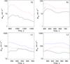 |
Fig. 7 Variation of velocity dispersions calculated over the whole domain in three temperature bands in the four models after kink instabilities. Model names are shown in panels. Black solid line is for the 0.25 MK <T< MK band, red dashed line is for 1 MK <T<4 MK, and blue dot-dashed line is for T> 4 MK. (There is practically no plasma with temperature >4 MK in models S1 and S2.) Lower limits of each time interval correspond approximately to the onset of kink instability and fast energy release. |
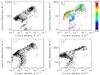 |
Fig. 8 Average n2-weighted velocity dispersions Δvnt versus current densities for the four models. Each dot represents a cube with the size of 2.5 L0 (2.5 Mm in smaller models and 10 Mm in larger models). Colour flags indicating the height corresponding to each dot are shown in the panel S2 to demonstrate correlation with the height. |
3.2. Characteristics of the velocity fields obtained from numerical models
The velocity dispersion functions Δvnt(T) have been calculated for each model for four regions (see Fig. 2): the large coronal region (practically, the whole domain volume above 2 Mm in models S1 and S2, and above 8 Mm in models L1 and L2), the loop-top region (a cube with the size of 3 Mm in S1 and S2, and 12 Mm in L1 and L2 containing the loop top), the footpoints (below 4 Mm in all four models), and for the whole domain. The values of Δvnt(T) are calculated separately using x-, y- and z-components of velocity. In the footpoint region, the z- and x- (or y-) componets of velocity correspond to directions along and across the magnetic field, respectively. At the same time, it is practically impossible to determine the dominant magnetic field direction in the large coronal sampling regions because of the twist and fast fluxtube motions. However, the dominant magnetic field direction can be determined for the loop-top regions. Additionally, we calculate the differential emission measure (DEM) functions for each model to show the distribution of the hot radiating plasma. The results are shown in Figs. 3–6. The times used here are arbitrary, and measured from restarts of simulations. In each model, fast energy release begins from the onset of kink instability, which happens approximately at 740 s in model S1, at 270 s in model S2, at 310 s in L1, and at 280 s in L2.
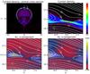 |
Fig. 9 Distributions of current density | j | and velocity deviations δv(x,z) around one of the energy release regions. Top left plot shows the global current density distribution at x = 0 plane and the location of the sampled region. Current density distribution and magnetic field lines in the selected region are shown in the top right panel. Distributions of the ρ2T-weighted velocity deviations (see text for details) are shown in the bottom left (x-component) and bottom right (z-component) panels. (Here the units of the current density colour scale are 3.6 × 10⁻³ A m-2 and the units of the ρ2T-weighted velocity colour scale are 2.8 × 10³ km s-1). Distances are in 106 m. |
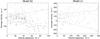 |
Fig. 10 Average velocity (Z-component) versus velocity dispersion for model S2 (left) and L2 (right). Each point corresponds to a sampling cube with side 2.25 Mm in the small model (left) and 9 Mm in the large model (right). Here, positive velocities correspond to plasma moving up, and vice versa (contrary to the convention used in most observational papers). |
The DEM functions for small models (Figs. 3, 4) can be divided into three parts. At low temperatures (0.1 MK) there is a peak corresponding to the relatively cold chromospheric plasma. It is followed by a nearly flat part and a peak at around 0.8–1.0 MK, corresponding to the coronal plasma. These two parts do not show substantial changes during loop evolution. The third part, at T> 1 MK, corresponds to the loop plasma heated during the reconnection. It is nearly flat, with slight positive slope during the reconnection phase and with slightly negative slope during the cooling phase. This part is limited by the peak temperature, which is about 2.5 MK for themodel S1 and about 3.5–4 MK for S2. The DEM functions corresponding to the larger models (Figs. 5, 6) can be divided into two parts: the bulk of the plasma forms a peak with a strong negative slope at a few MK, while the heated plasma shows exponential profiles up to the maximum temperature. The maximum temperature reached during the reconnection phase in model L1 is about 15–16 MK, while in the model L2 it is about 30 MK.
Figures 3–6 show LOS velocity dispersion as a functions of temperature, defined by Eq. (7). The values of Δvnt change substantially between different phases. They are of the order of 102 km s-1 during the reconnection and drop to ~10 km s-1 during the cooling phase. It can be seen that these values normally increase with the temperature in all regions in all considered models. Thus, the coronal parts of loops in small models demonstrate an increase in Δvnt from 10–30 km s-1 to about 100–200 km s-1 when the temperature increases from about 0.5–1 MK to 2–4 MK. In larger models, this value increases from 50–100 km s-1 at T ≈ 2–3 MK to 200–400 km s-1 around 20 MK. Smaller coronal sampling regions show a similar picture. The situation near the footpoints is more complicated. Overall, it is possible to say that in most cases the velocity dispersion is noticeably higher at higher temperatures. Thus, typically, inmodel S1 this velocity increases from few km s-1 below 1 MK to about 3–10 km s-1 at ≥1 MK. Similarly, inmodel S2, it also increases from few km s-1 just below 1 MK to about 10 km s-1 at ~2 MK. In large models, this velocity is even higher; it increases from about 10 km s-1 at 2–3 MK to about 50–100 km s-1 at 10–15 MK. However, near footpoints the Δvnt(T) distribution sometimes is flat or even decreasing.
Another interesting feature revealed by the non-thermal velocities near footpoints is the noticeable difference in dispersions in different directions. Thus, in the footpoints regions of smaller loops the Δvnt(T) distributions in x- and z-directions are similar at the beginning of reconnection. However, during the fastest stage of reconnection and during the cooling phase, the dispersion of vz is 3–4 higher higher than the dispersion of vx. Footpoints of larger loops show similar picture. Both during the fast reconnection and during cooling, the velocity dispersions in vertical direction are 2–3 times higher than those in horizontal directions. In other words, the velocity dispersion along the magnetic field is higher than that across the field.
A similar picture can be seen in the small sampling region near loop tops; dispersions of vy (direction along the loop) are higher than dispersions of vz (across the loop). In smaller loops this is the case at three different stages, however, in larger loops this contrast is small during the onset of reconnection, becoming very substantial (up to three times) towards the end of reconnection. This also might be explained as the effect of the magnetic field, particularly, towards the end of reconnection, when the azimuthal field is substantially reduced. There is no noticeable difference in the velocity dispersions in different directions for the whole coronal part or for the whole domain. This is natural, taking into account that there is no substantial mean magnetic field in these models.
It should be noted that the plots in the middle column in Figs. 3–6 corresponding to the footpoint regions sample substantially larger volumes (see Fig. 2). Their size is proportional to the domain (and loop) size and, therefore, in models L1 and L2 they sample larger volumes, including not only the chromosphere, but also the transition region and lower corona. This, most likely, explains why Δvnt(T) functions for footpoint and coronal regions are more similar in models L1 and L2, compared to models S1 and S2.
It should be noted that the non-thermal velocity dispersions near the footpoints, perhaps, are not representative of the whole loop; these velocity dispersions correspond to a cooler and more structured material of the chromosphere and transition region, where plasma β is higher and can be close to 1. However, they are still of interest. For instance, the variation of velocity dispersion with direction can indicate suppression or enhancement of the turbulence in a relatively strong magnetic field. At the same time, the coronal part represents the whole loop; its Δvnt(T) distributions are very similar to those of the whole domain.
Figure 7 shows the time variation of the velocity dispersion functions in three different temperature ranges, 0.25 MK–1 MK, 1 MK–4 MK, and >4 MK. There is practically no signal in the highest temperature band in small models S1 and S2. All four models show that Δvnt increases with temperature most of the time. Although, in model L1 values of Δvnt in 0.25 MK–1 MK and 1 MK–4 MK bands are nearly equal towards the end of reconnection, while in model L2 velocity dispersions in these bands are nearly equal just after the onset of reconnection.
In order to understand the relation between the primary energy release and velocity dispersions, we calculated Δvnt as functions of the current density j (Fig. 8). Similar to the temperature distribution of Δvnt, these function were calculated using the original spatial resolution of our MHD simulations (about 0.07 L0). Obtained Δvnt(j) functions did not show any noticeable spatial correlation between the velocity dispersions and current densities. However, when averaged over larger volumes (cubes with about 2.5 L0 size), the velocity dispersions clearly show spatial correlation with current densities (Fig. 8). Moreover, there is also a correlation with height. Thus, there are two types of hot regions in the considered models. Coronal plasma (see red, yellow, and green dots in Fig. 8, panel S2) shows weaker increase of the velocity dispersion with the current density (Δvnt ~ j0.35), while the hot regions in footpoint show a much steeper increase of Δvnt with currents (Δvnt ~ j). The effect of spatial resolution here can be explained by the structure of the primary energy release sites. Figure 9 shows the (x,z) distributions of current density and the velocity deviations and magnetic field lines around a region with high current density at the “current shield” formed just above the top of a twisted loop. Here, velocity deviations are calculated as  where index r means x, y, or z, and ρmean and Tmean are the density and temperature averaged over the sampled region, respectively. This region has all the basic features of the reconnection current sheet, including the inflow and outflow regions (see also Bareford et al. 2016). Importantly, plasma with high turbulent velocities is located in the exhaust regions, away from the current layer, and, hence, there is no immediate spatial correlation between the turbulent velocities and current density. However, the values of Δvnt averaged over volumes larger than these elementary current sheets shows spatial correlation with current densities.
On the other hand, relatively weak correlation and a substantial spread of points in the Δvnt versus | j | diagrams means that plasma turbulence and strong current are not always connected. Firstly, this is because several factors, which are not directly related to the energy release, can result in velocity dispersion (see Sect. 3.3). Secondly, the magnetic energy can be converted into kinetic energy of plasma turbulence well away from the reconnection regions. This is possible, for instance, if the plasma is heated and turbulised by MHD shocks generated by the magnetic reconnection, see Bareford & Hood (2015), Bareford et al. (2016).
We also compare the velocity dispersion (related to line width) with the bulk flow velocities (related to line shift); the measurements for our two models, S2 and L2 are shown in Fig. 10. They are calculated using Eqs. (6), (7) and integrated over temperature. Only plasma with temperatures higher than 1 MK is taken into account here. Each point corresponds to a cube with the side of about 30 grid points (2.25 Mm in model S2 and 9 Mm in L2). It is found that the average velocities are rather low when the non-thermal velocity dispersion is low, ⟨ v ⟩ ≈ 50 km s-1 when Δvnt = 20 km s-1. Then, it increases with Δvnt, reaching around ⟨ v ⟩ = 80–100 km s-1 for Δvnt ≈ 100 km s-1, and about ⟨ v ⟩ = 700 km s-1 for Δvnt ≈ 1000 km s-1. Both negative and positive average velocities are present and the dependences between Δvnt and ⟨ v ⟩ can be linearly approximated both for upflows and downflows. Although these dependences are clearly visible on the graphs, the spread of points is very big (several km s-1).
3.3. Comparison with observations and discussion
Our models can reproduce the two key observational features described in Sect. 1. Firstly, similarly to observational data, the non-thermal velocity dispersion in the model increases with temperature, at least in its coronal part (which is most of the volume for most loops). The exact values depend substantially on the model (or loop) size. At temperatures of about 1 MK, these velocity dispersions are about 10–50 km s-1, increasing to about 100–200 km s-1 at temperatures of 5–10 MK and reaching up to 500 km s-1 in the range of 20–30 MK. Observational data (see Sect. 1) similarly shows an increase from 10–20 km s-1 at ~1 MK to few hundreds of km s-1 at about 10 MK. Also, similar to observational data, our models show a noticeable peak in Δvnt(T) functions at low temperatures of around 0.3–0.5 MK.
Secondly, the loops considered in our models also demonstrate the correlation of the bulk velocity with non-thermal velocity dispersion: the higher the LOS flow velocity, the higher is the Δvnt value. Both, downflows and upflows are present (nearly equally). However, the average LOS velocities derived from our models demonstrate a substantial spread of about 100 km s-1, while in the observations the ⟨ v ⟩ distribution is more compact (Doschek et al. 2008). This spread is larger in the plasma with positive velocities (upflow). Finally, the range of average LOS velocities obtained in our simulations is considerably larger (up to 800 km s-1) than in the observations by Doschek mentioned above. However, these values are still acceptable as such velocities are sometimes observed in the larger loop (Cirtain et al. 2013).
The correlation between temperature and velocities is not surprising. Indeed, one would expect that plasma with more heating would contain more kinetic energy in form of large-scale turbulence and regular flows. Thus, in our simulation the highest velocities appear in and around the energy release regions (close to the loop top, and in loop legs closer to current concentrations near footpoints). This also explains the correlation between the velocity dispersion and the average flow velocity. Indeed, both values ⟨ v ⟩ and Δvnt are high in the hot plasma regions, relatively low in colder regions of the flaring loop, and very low outside the loop. Generally, it means that a single energy release mechanism is responsible for small-scale turbulent velocities and large-scale plasma motion, so that the energies of these two types of motion are proportional to each other. The reason why the spread in velocities obtained in our simulations (Fig. 10) is substantially greater than in observations is less clear. This may be because the large box we use in our measurements includes very different regions. On the other hand, it may be because in observations the values of ⟨ v ⟩ and Δvnt are calculated over a larger temperature range than in our simulations.
It is important to note that there are several different factors resulting in velocity dispersion, and some of these factors may be unrelated to the energy release. The key factor, which is in the focus of this paper, is the turbulence in the very hot flaring plasma. As shown in the Sect. 3.2, this turbulence occurs in the very hot plasma ejected from elementary reconnecting current sheets. Since the reconnection is the most powerful heating mechanism in our models, this mechanism would be dominant at high temperatures (1 MK and higher). Secondly, there are fast chaotic motions due to the loop kinking after the instability. Since these velocities should be highest close to the loop top, loop kinking would affect the temperature range >0.5 MK, i.e. the temperature of the quiet coronal plasma and the temperature of flaring plasma. There is also an important implication from this mechanism, which is that noticeable non-thermal velocity dispersions may appear even before the heating, as is found in the observations (Harra et al. 2013). Thirdly, the thermal flux from the corona can heat dense transition regions and the chromosphere, which may add to the velocity dispersion at lower temperatures 104–106 K via non-uniform evaporation upflows.
Substantial difference in the velocity dispersions in different directions can be explained assuming that the mean magnetic field is close to the loop direction. (Here, by the loop direction we mean the skeleton line of a loop going from one footpoint to another footpoint via the loop top.) This would mean that the velocity dispersion along the mean magnetic field is higher than across the magnetic field. There are two factors that could lead to this. Firstly, the turbulence in the hot flaring plasma can be anisotropic since it is stronger along the mean field. Secondly, since the hot plasma is moving predominantly along magnetic field, any cross-field inhomogeneity of the flow velocity at small spatial scales results in LOS velocity dispersion, if observed along the magnetic field direction. This inhomogeneity is possible because of the anisotropic thermal conduction; heat is quickly redistributed along magnetic field lines with almost no conduction in the perpendicular direction.
Finally, there are two features in the velocity field unrelated to the instability and the energy release: footpoint rotation and kink oscillations of the loops before the instability. Thus, slow periodic variation in the total kinetic energy in these loops (see e.g. Fig. 4 in Gordovskyy et al. 2014) are likely to be due to low-amplitude fundamental mode (i.e. N = 1) kink oscillations. Based on the kinetic energy variation, their amplitude should be of the order of 0.001v0 or smaller (i.e. about 1 km s-1 or smaller). Hence, these oscillations, in principle, could make a small contribution to the velocity dispersions, particularly at low temperatures. The maximum linear speed due to the loop rotation is about 0.004v0, or 10 km s-1. This motion also can contribute to the velocity dispersion, especially at low temperatures (since the velocity dispersion is n2-weighed and the temperatures in the dense chromosphere are 104–105 K. However, the velocity dispersions higher than ~10 km s-1 cannot be attributed to the driver.
4. Summary
In the present work, we derive characteristics of the velocity field in flaring loops and compare them with observations, focusing on the plasma velocity dispersions, which correspond to non-thermal broadening of coronal EUV lines. It is found that our models yield velocity dispersions and average LOS velocities, which are in qualitative and quantitative agreement with those derived from observational data.
Thus, velocity dispersions Δvnt, average LOS velocities ⟨ v ⟩ and maximum temperature depend on the flare size and characteristic magnetic field in the loop. Thus, in small loops (with length of about 20 Mm) the maximum temperature varies between 2 MK (loop with footpoint magnetic field about 100 G) and 4 MK (footpoint field 200 G), average velocities and velocity dispersions are about 10–100 km s-1. In large loops (with length of about 80 Mm) the temperature can reach 16 MK (footpoint field 700 G) and 30 MK (footpoint field 1.5 kG), while the average velocities and velocity dispersions are 50–500 km s-1.
In the chromospheric and photospheric plasma close to footpoints the velocity dispersion is low at about 5–20 km s-1. The velocity dispersion along the field is found to be lower, by factor of 2–4, than that across the magnetic field.
The velocity dispersion correlates with temperature. Thus, it is around 10 km s-1 near T ≈ 0.5–1.0 MK, increases to about 100 km s-1 at ~2 MK, and reaches about 200–500 km s-1 at T ≈ 10–20 MK. The velocity dispersions show spatial correlation with current densities, and they vary approximately as Δvnt ~ j0.35 in the corona, and as Δvnt ~ j near footpoints. Velocity dispersions appear to be higher along the loop direction, both near the footpoints and at the loop tops. Typically, the ratio is about 2–4. Finally, the velocity dispersion correlates with average LOS velocity. Average velocities can be both positive and negative (upflow and downflow). At lower Δvnt values these two quantities are connected approximately as ⟨ v ⟩ ≈ Δvnt, while at high values Δvnt ≥ 100 km s-1 this relation is ⟨ v ⟩ ≈ 0.3Δvnt for upflow and ⟨ v ⟩ ≈ 0.6Δvnt for downflow.
Therefore, based on our simulations, we can conclude that the correlation between the observed velocity dispersions (derived from spectral line widths) and the temperature, and the correlation between the average LOS velocities (derived from spectral line shifts) and the velocity dispersions, indicate that a single mechanism, direct plasma heating during magnetic reconnection, is responsible both for turbulisation of plasma and bulk plasma motion.
It is important to say that a good agreement with observations does not mean that all flares investigated in the observational studies (mentioned in Sect. 1) occurred in twisted coronal loops. However, the fact that solar flares occurring in this type of magnetic configurations produces data similar to observations implies that the “twisted loop” configuration is a viable model for a solar flare, which can explain observations of ⟨ v ⟩ and Δvnt using simple reconnection scenario with multiple extended reconnection regions.
Acknowledgments
This work is funded by Science and Technology Facilities Council (UK) (STFC). MHD simulations have been performed using UKMHD facilities in the University of St Andrews and DIRAC system at Durham University, operated by the Institute for Computational Cosmology on behalf of the STFC DiRAC HPC Facility (http://www.dirac.ac.uk). DiRAC is part of the National E-Infrastructure.
References
- Antolin, P., & Rouppe van der Voort, L. 2012, ApJ, 745, 152 [NASA ADS] [CrossRef] [Google Scholar]
- Arber, T. G., Longbottom, A. W., Gerrard, C. L., & Milne, A. M. 2001, J. Comp. Phys, 171, 151 [Google Scholar]
- Bareford, M. R., & Hood, A. W. 2015, Phil. Trans. Roy. Soc. A. 373, 20140266 [NASA ADS] [CrossRef] [Google Scholar]
- Bareford, M. R., Hood, A. W., & Browning, P. K. 2013, A&A, 550, A40 [NASA ADS] [CrossRef] [EDP Sciences] [Google Scholar]
- Bareford, M. R., Gordovskyy, M., Browning, P. K., & Hood, A. W. 2016, Sol. Phys., 291, 187 [NASA ADS] [CrossRef] [Google Scholar]
- Baty, H., & Heyvaers, J. 1996, A&A, 308, 935 [NASA ADS] [Google Scholar]
- Benz, A. O. 2008, Liv. Rev. Sol. Phys., 5 [Google Scholar]
- Botha, G. J. J., Arber, T. D., & Srivastava, A. K. 2012, ApJ, 745, 53 [NASA ADS] [CrossRef] [Google Scholar]
- Braginskii, S. I. 1965, Rev. Plasma Phys., 1, 205 [NASA ADS] [Google Scholar]
- Browning, P. K., & Lazarian, A. 2013, Space Sci. Rev., 178, 325 [NASA ADS] [CrossRef] [Google Scholar]
- Browning, P. K., & Van der Linden, R. A. M. 2003, A&A, 400, 355 [NASA ADS] [CrossRef] [EDP Sciences] [Google Scholar]
- Browning, P. K., Gerrard, C., Hood, A. W., Kevis, R., & Van der Linden, R. A. M. 2008, A&A, 485, 837 [NASA ADS] [CrossRef] [EDP Sciences] [Google Scholar]
- Cirtain, J. W., Golub, L., Winebarger, A. R., et al. 2013, Nature, 493, 501 [NASA ADS] [CrossRef] [Google Scholar]
- Culhane, J. L., Harra, L. K., James, A. M., et al. 2007, Sol. Phys., 243, 19 [Google Scholar]
- Del Zanna, G. 2008, A&A, 481, L49 [NASA ADS] [CrossRef] [EDP Sciences] [Google Scholar]
- Del Zanna, G., Mitra-Kraev, U., Bradshaw, S. J., Mason, H. E., & Asai, A. 2011, A&A, 526, A1 [NASA ADS] [CrossRef] [EDP Sciences] [Google Scholar]
- Doschek, G. A., Mariska, J. T., Warren, H. P., et al. 2007, ApJ, 667, L109 [NASA ADS] [CrossRef] [Google Scholar]
- Doschek, G. A., Warren, H. P., Mariska, J. T., et al. 2008, ApJ, 686, 1362 [NASA ADS] [CrossRef] [Google Scholar]
- Doschek, G. A., Warren, H. P., & Young, P. R. 2013, ApJ, 767, 55 [NASA ADS] [CrossRef] [Google Scholar]
- Emslie, A. G., Kucharek, H., Dennis, B. R., et al. 2004, J. Geophys. Res., 109, 10104 [NASA ADS] [CrossRef] [Google Scholar]
- Fleishman, G. D., Nita, G. M., & Garry, D. E. 2015, ApJ, 802, 122 [NASA ADS] [CrossRef] [Google Scholar]
- Gordovskyy, M., & Browning, P. K. 2012, Sol. Phys., 277, 299 [NASA ADS] [CrossRef] [Google Scholar]
- Gordovskyy, M., & Lozitsky, V. G. 2014, Sol. Phys., 289, 3681 [NASA ADS] [CrossRef] [Google Scholar]
- Gordovskyy, M., Browning, P. K., Kontar, E. P., & Bian, N. H. 2013, Sol. Phys., 284, 489 [NASA ADS] [CrossRef] [Google Scholar]
- Gordovskyy, M., Browning, P. K., Kontar, E. P., & Bian, N. H. 2014, A&A, 561, A72 [NASA ADS] [CrossRef] [EDP Sciences] [Google Scholar]
- Harra, L. K., Matthews, S., Culhane, J. L., et al. 2013, ApJ, 774, 122 [NASA ADS] [CrossRef] [Google Scholar]
- Hood, A. W., & Priest, E. R. 1979, Sol. Phys., 64, 303. [NASA ADS] [CrossRef] [Google Scholar]
- Hood, A. W., Browning, P. K., & Van der Linden, R. A. M. 2009, A&A, 506, 913 [NASA ADS] [CrossRef] [EDP Sciences] [Google Scholar]
- Hubeny, I., & Mihalas, D. 2014, Theory of stellar atmospheres (Princeton Uni. Press) [Google Scholar]
- Klimchuk, J. A., Patsourakos, S., & Cargill, P. A. 2008, ApJ, 682, 1351 [Google Scholar]
- Ko, Y.-K., Raymond, J. C., Vrsnak, B., & Vujic, E. 2010, ApJ, 722, 625 [NASA ADS] [CrossRef] [Google Scholar]
- Kontar, E. P., Dickson, E., & Kasparova, J. 2008, Sol. Phys., 252, 139 [NASA ADS] [CrossRef] [Google Scholar]
- Lazarian, A., & Vishniak, E. T. 1999, ApJ, 517, 700 [NASA ADS] [CrossRef] [Google Scholar]
- Lemen, J. R., Title, A. M., Akin, D. J., et al. 2012, Sol. Phys., 275, 17 [NASA ADS] [CrossRef] [Google Scholar]
- Pinto, R., Gordovskyy, M., Browning, P. K., & Vilmer, N. 2016, A&A, 585, A159 [NASA ADS] [CrossRef] [EDP Sciences] [Google Scholar]
- Susino, R., Bemporad, A., & Krucker, S. 2013, ApJ, 777, 93 [NASA ADS] [CrossRef] [Google Scholar]
- Vrsnak, B., Poletto, G., Vujic, E., et al. 2009, ApJ, 499, 905 [Google Scholar]
- Watanabe, T., Hara, H., Sterling, A. C., & Harra, L. K. 2010, ApJ, 719, 213 [NASA ADS] [CrossRef] [Google Scholar]
- Young, P. R., Doschek, G. A., Warren, H. P., & Hara, H. 2013, ApJ, 766, 127 [NASA ADS] [CrossRef] [Google Scholar]
All Figures
|
Fig. 1 Evolution of Model L1. Left column: magnetic field lines; red and blue field lines are tied to opposite footpoints of the twisted loop; yellow lines denote ambient field. Middle column: temperature distribution; yellow patchy surface corresponds to 2 MK; orange and blue surfaces correspond to 3 and 4 MK, respectively. Right column: surfaces of j = jcrit, i.e. showing the locations with fast magnetic energy release. Times (after onset of the instability) are shown for each row on the left in units of characteristic Alfvén times tA, which are 0.44 s for this model. |
| In the text | |
|
Fig. 2 Locations of sampling boxes in the domain: green box denotes the footpoint region, red box denotes the coronal region, and the blue box denotes the loop-top region. For models S1 and S2 the units are 1 Mm, while for larger models L1 and L2 the units are 4 Mm. |
| In the text | |
|
Fig. 3 Model S1. Left column: differential emission measure versus temperature for the whole domain. Middle column: average n2-weighted velocity dispersions Δvnt(T) (calculated as |
| In the text | |
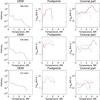 |
Fig. 4 Same as in Fig. 3, but for Model S2. |
| In the text | |
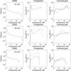 |
Fig. 5 Same as in Fig. 3, but for large-scale Model L1. |
| In the text | |
 |
Fig. 6 Same as in Fig. 3, but for large-scale Model L2. |
| In the text | |
|
Fig. 7 Variation of velocity dispersions calculated over the whole domain in three temperature bands in the four models after kink instabilities. Model names are shown in panels. Black solid line is for the 0.25 MK <T< MK band, red dashed line is for 1 MK <T<4 MK, and blue dot-dashed line is for T> 4 MK. (There is practically no plasma with temperature >4 MK in models S1 and S2.) Lower limits of each time interval correspond approximately to the onset of kink instability and fast energy release. |
| In the text | |
|
Fig. 8 Average n2-weighted velocity dispersions Δvnt versus current densities for the four models. Each dot represents a cube with the size of 2.5 L0 (2.5 Mm in smaller models and 10 Mm in larger models). Colour flags indicating the height corresponding to each dot are shown in the panel S2 to demonstrate correlation with the height. |
| In the text | |
|
Fig. 9 Distributions of current density | j | and velocity deviations δv(x,z) around one of the energy release regions. Top left plot shows the global current density distribution at x = 0 plane and the location of the sampled region. Current density distribution and magnetic field lines in the selected region are shown in the top right panel. Distributions of the ρ2T-weighted velocity deviations (see text for details) are shown in the bottom left (x-component) and bottom right (z-component) panels. (Here the units of the current density colour scale are 3.6 × 10⁻³ A m-2 and the units of the ρ2T-weighted velocity colour scale are 2.8 × 10³ km s-1). Distances are in 106 m. |
| In the text | |
|
Fig. 10 Average velocity (Z-component) versus velocity dispersion for model S2 (left) and L2 (right). Each point corresponds to a sampling cube with side 2.25 Mm in the small model (left) and 9 Mm in the large model (right). Here, positive velocities correspond to plasma moving up, and vice versa (contrary to the convention used in most observational papers). |
| In the text | |
Current usage metrics show cumulative count of Article Views (full-text article views including HTML views, PDF and ePub downloads, according to the available data) and Abstracts Views on Vision4Press platform.
Data correspond to usage on the plateform after 2015. The current usage metrics is available 48-96 hours after online publication and is updated daily on week days.
Initial download of the metrics may take a while.