| Issue |
A&A
Volume 588, April 2016
|
|
|---|---|---|
| Article Number | A45 | |
| Number of page(s) | 14 | |
| Section | Interstellar and circumstellar matter | |
| DOI | https://doi.org/10.1051/0004-6361/201526845 | |
| Published online | 16 March 2016 | |
Magnetic field geometry of an unusual cometary cloud Gal 110-13
1 Aryabhatta Research Institute of Observational Sciences (ARIES), 263002 Nainital, India
e-mail: This email address is being protected from spambots. You need JavaScript enabled to view it.
2 Pt. Ravishankar Shukla University, 492010 Raipur, India
3 Korea Astronomy & Space Science Institute (KASI), 776 Daedeokdae-ro, Yuseong-gu, Daejeon, Republic of Korea
4 University of Science Technology, 217 Gajungro, Yuseong-gu, 305-333 Daejeon, Republic of Korea
5 Indian Institute of Space Science and Technology (IIST), 695547 Trivandrum, India
Received: 28 June 2015
Accepted: 19 October 2015
Abstract
Aims. We carried out optical polarimetry of an isolated cloud, Gal 110-13, to map the plane-of-the-sky magnetic field geometry. The main aim of the study is to understand the most plausible mechanism responsible for the unusual cometary shape of the cloud in the context of its magnetic field geometry.
Methods. When unpolarized starlight passes through the intervening interstellar dust grains that are aligned with their short axes parallel to the local magnetic field, it gets linearly polarized. The plane-of-the-sky magnetic field component can therefore be traced by doing polarization measurements of background stars projected on clouds. Because the light in the optical wavelength range is most efficiently polarized by the dust grains typically found in the outer layers of the molecular clouds, optical polarimetry enables us to trace the magnetic field geometry of the outer layers of the clouds.
Results. We made R-band polarization measurements of 207 stars in the direction of Gal 110-13. The distance of Gal 110-13 was determined as ~450 ± 80 pc using our polarization and 2MASS near-infrared data. The foreground interstellar contribution was removed from the observed polarization values by observing a number of stars located in the vicinity of Gal 110-13 which has Hipparcos parallax measurements. The plane-of-the-sky magnetic field lines are found to be well ordered and aligned with the elongated structure of Gal 110-13. Using structure function analysis, we estimated the strength of the plane-of-the-sky component of the magnetic field as ~25 μG.
Conclusions. Based on our results and comparing them with those from simulations, we conclude that compression by the ionization fronts from 10 Lac is the most plausible cause of the comet-like morphology of Gal 110-13 and of the initiation of subsequent star formation.
Key words: ISM: clouds / polarization / ISM: magnetic fields / ISM: individual objects: Gal 110-13
© ESO, 2016
1. Introduction
Gal 110-13, also known as LBN 534 or DG 191, is an isolated, unusually elongated, comet-shaped molecular cloud located at the galactic coordinate l = 110° & b = −13°. The cloud belongs to the Andromeda constellation. First recognized by Whitney (1949), the Gal 110-13 cloud consists of a blue reflection nebula, vdB 158, located at the southern end of the cloud, which is illuminated by a B-type star, HD 222142. Based on the spectroscopic parallaxes determined for HD 222142 and another B-type star, HD 222086, Aveni & Hunter (1969) derived a distance of 440 ± 100 pc to the cloud. Using 100 μm IRAS data, Odenwald & Rickard (1987) identified and listed 15 isolated clouds that showed cometary or filamentary morphology. The remarkable comet-like morphology of Gal 110-13 makes it one of the most unusual and isolated clouds in the list by Odenwald & Rickard (1987). The cloud major axis, which is ~1° in extent, is oriented at a position angle of ~45° to the east with respect to the north. The cloud has a width of ~8′.
Odenwald et al. (1992) made a detailed study of Gal 110-13 multiwavelength observations. They found the cloud, especially the tail part, to be highly clumpy in nature. They explored possible mechanisms (such as the interaction of the cloud with ionization fronts or supernova remnants, gravitational instability, hydrodynamics process involving gas stripping, and the cloud-cloud collision) that could explain the unusual shape of the cloud. Of these, according to Odenwald et al. (1992), the cloud-cloud collision mechanism was considered to be the most plausible one. Gal 110-13 is explained to have formed as a consequence of collision between two interstellar clouds whose compression zone resulted in the elongated far-IR and 12CO emission detected from the cloud. However, because Gal 110-13 is roughly pointing toward the Lac OB association, Lee & Chen (2007) suggest that the present morphology of the cloud could also be explained by its interaction with supernova blast waves or ionization fronts from the massive members of the Lac OB association. A comet-like morphology of clouds is formed when a supernova explosion shocks a pre-existing spherical cloud and compresses it to form the head, and the blast wave drives the material mechanically away from the supernova to form the tail (Brand et al. 1983). Reipurth (1983) suggested that the UV radiation from massive stars photoionizes a pre-existing spherical cloud, and shock fronts compress it to form the head. The tail is formed either from the eroded material of the cloud or the pre-existing medium protected from the UV radiation because of the shadowing of the tail by the head.
Several analytical and numerical hydrodynamics studies have been carried out to understand the dynamical behavior of the collision between interstellar clouds (Stone 1970a,b; Hausman 1981; Gilden 1984; Lattanzio et al. 1985; Keto & Lattanzio 1989; Habe & Ohta 1992; Kimura & Tosa 1996; Ricotti et al. 1997; Miniati et al. 1997; Klein & Woods 1998; Marinho & Lépine 2000; Anathpindika 2009, 2010; Takahira et al. 2014) and a dense, isolated cloud that is illuminated from one side by a source of ionizing radiation (Bertoldi 1989; Bertoldi & McKee 1990; Sandford et al. 1992; Lefloch & Lazareff 1994, 1995; Williams et al. 2001; Kessel-Deynet & Burkert 2003; Mizuta et al. 2005; Miao et al. 2009; Gritschneder et al. 2010; Mackey & Lim 2010; Tremblin et al. 2012). In recent years, a number of studies have been conducted to address the role played by the magnetic field in the cloud-cloud collision scenario (e.g., Marinho et al. 2001) and in the external ionization-induced evolution of an isolated globule (e.g., Henney et al. 2009). In both these processes, the magnetic field seems to alter the results from the hydrodynamical evolution significantly.
Based on 3D-smoothed particle magnetohydrodynamics simulations (3D-SPMHD, Marinho et al. 2001), it was shown that in a cloud-cloud collision scenario the clump formation is only possible in the case where the collision happens between two identical spherical clouds that are traveling parallel to the magnetic field orientation. After the collision, the field lines are found to be chaotic on the cloud scale (~few pc) though a coherence in the field distribution was found on the clump scale (≲0.5 pc). The evolution of globules under the influence of ionizing radiation from an external source was studied using 3D-radiation magnetohydrodynamics simulations (Henney et al. 2009; Mackey & Lim 2011). The studies show that a strong (~150–180 μG) initially uniform magnetic field perpendicular to the direction of the ionizing radiation remained unchanged, thus altering the dynamical evolution of the globule significantly from the non-magnetic case. In contrast, weak or medium, initially perpendicular magnetic field lines are swept into alignment with the direction of the ionization radiation and the long axis of the globule during the evolution. The magnetic field parallel to the direction of the ionizing radiation, however, are found to remain unchanged producing a broader and snubber globule head. Irrespective of the initial magnetic field orientation, the field lines are found to be ordered well in the external radiation-induced evolution of globules. Such well-ordered magnetic field lines are observed in a number of cometary globules (e.g., Sridharan et al. 1996; Bhatt 1999; Bhatt et al. 2004; Targon et al. 2011; Soam et al. 2013). Therefore, we expect that the geometry of the magnetic field lines in Gal 110-13 provide useful information on the possible mechanism that might have been responsible for forming the cloud.
Observations of polarized radiation in the interstellar medium at optical-through-millimeter wavelengths have been attributed to extinction by, and emission from, interstellar dust grains (Hiltner 1949, 1951; Hildebrand 1988). The polarization measurements in optical (e.g., Vrba et al. 1976; Goodman et al. 1990; Alves et al. 2008; Soam et al. 2013; Alves et al. 2014), near-infrared (e.g., Goodman et al. 1995; Chapman et al. 2011; Sugitani et al. 2011; Clemens 2012; Cashman & Clemens 2014; Bertrang et al. 2014; Kusune et al. 2015; Alves et al. 2014) and submillimeter-millimeter wavelengths (e.g., Rao et al. 1998; Dotson et al. 2000, 2010; Vaillancourt & Matthews 2012; Hull et al. 2014; Alves et al. 2014) are used to map the magnetic field geometry of molecular clouds. Optical polarization position angles trace the plane of the sky orientation of the ambient magnetic field at the periphery of the molecular clouds (with AV~ 1–2 mag; Goodman et al. 1995; Goodman 1996). In this work, we present the optical polarization measurements of 207 stars projected on Gal 110-13 to map the projected magnetic field geometry of the cloud. We present the details of the observations and data reduction in Sect. 2. In Sect. 3, we present the results obtained from the observations and in Sect. 4 discuss the results. We conclude the paper with a summary presented in Sect. 5.
2. Observations and data reduction
The optical linear polarization observations of the region associated with Gal 110-13 were carried out with the ARIES IMaging POLarimeter (AIMPOL), mounted at the f/13 Cassegrain focus of the 104-cm Sampurnanand telescope of ARIES, Nainital, India. It consists of a field lens in combination with the camera lens (85mm, f/1.8); in between them, an achromatic, rotatable half-wave plate (HWP) are used as modulator and a Wollaston prism beam-splitter as analyzer. A detailed description of the instrument and the techniques of the polarization measurements may be found in Rautela et al. (2004). We used a standard Johnson RKC filter (λeff = 0.760 μm) photometric band for the polarimetric observations. The plate scale of the CCD is 1.48′′/pixel and the field of view is ~8′ in diameter. The full width at half maximum (FWHM) varies from two to three pixels. The read-out noise and the gain of the CCD are 7.0 e-1 and 11.98 e-1/ADU, respectively. The log of the observations is presented in Table 1.
Log of observations.
We used the Image Reduction and Analysis Facility (IRAF) package to perform standard aperture photometry to extract the fluxes of ordinary (Io) and extraordinary (Ie) rays for all the observed sources with a good signal-to-noise ratio. When the HWP is rotated by an angle α, then the electric field vector rotates by an angle 2α. A ratio R(α) has been defined as follows:  (1)where P is the fraction of the total linearly polarized light, and θ the polarization angle of the plane of polarization. Since α is the position of the fast axis of the HWP at 0°, 22.5°, 45° and 67.5° corresponding to the four normalized Stokes parameters, respectively, q [R(0°)], u [R(22.5°)], q1 [R(45°)] and u1 [R(67.5°)]. Because the polarization accuracy is, in principle, limited by the photon statistics, the errors in normalized Stokes parameters σR(α) (σq, σu, σq1 and σu1 in percent) are estimated using the expression (Ramaprakash et al. 1998)
  (2)where No and Ne are the number of photons in ordinary and extraordinary rays, respectively, and Nb[=(Nbe + Nbo)/2] is the average background photon counts in the vicinity of the extraordinary and ordinary rays.
Standard stars with zero polarization were observed during each run to check for any possible instrumental polarization. The typical instrumental polarization is found to be less than 0.1%. The instrumental polarization of AIMPOL on the 104-cm Sampurnanand telescope has been monitored since 2004 for various observing programs and found to be stable. Two polarized standard stars HD 236633 and BD+59°389 chosen from Schmidt et al. (1992) were observed on every observing run to determine the reference direction of the polarizer. In addition another polarized standard star HD 19820 was also observed for two nights. The results obtained for the standard stars are presented in Table 2. The polarization values for the standard stars given in Schmidt et al. (1992) were obtained with the Kron-Cousins R filter. We corrected for the instrumental polarization from the observed degree of polarization and for the zero point offset using the offset between the standard polarization position angle values obtained by observation and those given in Schmidt et al. (1992).
Polarized standard stars observed inRkc band.
3. Results
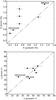 |
Fig. 1 Comparison of the degree of polarization (upper panel) and the position angles (lower panel) of the seven stars found in common with those observed by Grinin et al. (1995). |
The results of our R-band polarimetry of 207 stars toward Gal 110-13 are presented in Table A.1. We tabulated the results of only those sources that have the ratio of the degree of polarization (P%) and error in the degree of polarization (σP), P/σP ≥ 2. The columns of the Table A.1 show the star identification number in increasing order of their right ascension, the declination, measured P (%) and polarization position angles (θP in degrees). The mean value of P is found to be 1.5%. The mean value of θP obtained from a Gaussian fit to the distribution is found to be 45°. The standard deviation in P and θP is found to be 0.8% and 12°, respectively. A total of ten stars were observed by Grinin et al. (1995) toward the Gal 110-13 region. Of these, seven sources are found to be in common. In Fig. 1, we compare our results with those from the Grinin et al. (1995) obtained in R filter. The effective wavelength of the R filter used is not mentioned in the paper. The degree of polarization obtained by Grinin et al. (1995) is found to be systematically higher. Two sources, BM And and HD 222142 are identified and labeled. BM And is classified as a classical T Tauri-type star (Herbig & Bell 1988). This star is known for its photometric and polarimetric variability (Grinin et al. 1995). HD 222142 which is associated with the reflection nebulosity could also be a variable source.
4. Discussion
Unpolarized starlight when propagates through interstellar dust grains that are elongated and somehow partially aligned by the interstellar magnetic field, becomes linearly polarized. It appears that the grains are aligned with their shortest axes parallel to the magnetic field direction (Davis & Greenstein 1951; Lazarian 2007; Hoang & Lazarian 2014; Alves et al. 2014). The polarization is produced because of the preferential extinction of one linear polarization mode relative to the other. The polarization measured this way gets contributions from all the dust grains that are present in the pencil beam (since a star is a point source) along a line of sight. To obtain the polarization due to the dust grains that are present in the cloud, it is essential to subtract the polarization due to those that are present foreground to the cloud. But to subtract the foreground contribution, the distance of the cloud should be known beforehand.
4.1. The distance
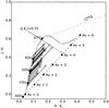 |
Fig. 2 (J−H) vs. (H−Ks) CC diagram drawn for stars (with AV ≥ 1) from the region containing Gal 110-13 to illustrate the method. The solid curve represents locations of unreddened main sequence stars. The reddening vector for an A0V type star drawn parallel to the Rieke & Lebofsky (1985) interstellar reddening vector is shown by the dashed line. The locations of the main sequence stars of different spectral types are marked with square symbols. The region to the right of the reddening vector is known as the near infrared excess region and corresponds to the location of pre-main sequence sources. The dash-dot-dash line represents the loci of unreddened CTTSs (Meyer et al. 1997). The open circles represent the observed colours, and the arrows are drawn from the observed to the final colours obtained by the method for each star. |
The distance to Gal 110-13 was determined by Aveni & Hunter (1969) by estimating spectroscopic parallaxes of two B-type stars, HD 222142 (source illuminating the reflection nebula, vdB 158) and HD 222086. They derived a distance of 440 ± 100 pc to the cloud. However, based on the Hipparcos parallax measurements of HD 222086 (van Leeuwen 2007), the distance to the star is ~640 ± 380 pc. No other distance estimates are available for Gal 110-13 in the literature. We made an attempt to determine the distance to Gal 110-13 using homogeneous JHKs photometric data produced by the Two Micron All Sky Survey (2MASS, Cutri et al. 2003). This is based on a method in which spectral classification of stars projected on the fields containing the clouds are made into main sequence and giants using the J−H and H−Ks colors (Maheswar et al. 2010). In this technique, first the observed J−H and H−Ks colors of the stars with (J−Ks) ≤0.751 and photometric errors in JHKs≤ 0.03 magnitude are dereddened simultaneously using trial values of AV and a normal interstellar extinction law (Rieke & Lebofsky 1985). The best fit of the dereddened colors to those intrinsic colors giving a minimum value of χ2 then yielded the corresponding spectral type and AV for the star. The main sequence stars, thus classified, are plotted in an AV versus distance diagram to bracket the cloud distance (e.g., Maheswar et al. 2010, 2011; Eswaraiah et al. 2013; Soam et al. 2013). The pictorial description of the method, given in detail in Maheswar et al. (2010), is presented in the near infrared color-color diagram for the stars chosen from the region containing the cloud Gal 110-13 (Fig. 2). The extinction vector of an A0V star for increasing values of AV and a normal interstellar extinction law is shown. Extinction values estimated for A0V stars would set the upper limit, and as we move toward more late-type stars, the extinction values traced would decrease in our method.
Any erroneous classifications of giants as dwarfs could result in underestimating their distance, which could lead to uncertainty in any estimation of the distance to the cloud. This problem was resolved by dividing the field containing a cloud into subfields. While the rise in the extinction due to the presence of a cloud should occur almost at the same distance in all the fields, if the whole cloud is located at same distance, the incorrectly classified stars in the subfields would show high extinction not at same but at random distances. In case of clouds that have smaller angular sizes, other spatially associated clouds that show similar radial velocities could be selected. Here the assumption is that the clouds that are spatially associated and located at similar distances, have similar velocities.
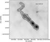 |
Fig. 3 2° × 2° Planck 857 GHz image of Gal 110-13. The circles represent the positions of those sources that are plotted (closed circles) in the AV vs. distance plot (Fig. 4). |
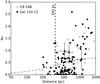 |
Fig. 4 AV vs. distance plot for the regions containing Gal 110-13 (closed circles) and CB 248 (open circles). The dashed vertical line is drawn at 345 pc inferred from the procedure described in Maheswar et al. (2010). The dash-dotted curve represents the increase in the extinction towards the Galactic latitude of b = −13° as a function of distance produced from the expressions given by Bahcall & Soneira (1980). Typical error bars are shown on a few data points. |
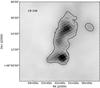 |
Fig. 5 1° × 1° Planck 857 GHz image of CB 248. The circles represent the positions of those sources that are shown in the AV vs. distance plot (open circles in Fig. 4). |
In Fig. 3, we show the stars that are lying within the cloud boundary, identified based on the Planck 857 GHz flux, and that are used for estimating the distance of Gal 110-13. The AV −distance plot of these stars are shown in Fig. 4, along with the change in the extinction as a function of distance toward the Galactic latitude of b = −13° produced using the expressions given by Bahcall & Soneira (1980). An abrupt increase in the values of extinction, values which are significantly above those expected from the expressions by Bahcall & Soneira (1980), is noticed for sources lying beyond ~350 pc. A number of sources lying close to ~200 pc also show a slight increase in the extinction value.
Based on the 21-cm line observations, Cappa de Nicolau & Olano (1990) found three main components having LSR-velocities (VLSR) of about 0 to +4 km s-1, −12 to −3 km s-1 and −30 to −20 km s-1 in the spectra of the region 88° ≤ l ≤ 106° and −26° ≤ b ≤ −10°. On account of their spatial distribution, Cappa de Nicolau & Olano (1990) suggested that all the three components are related to the region and explained in terms of expansion of a shell of neutral and molecular gas centered at l = 99° and b = −12°.5. The radial velocity of 10 Lac (nearest O-type star) is found to be −9.7 km s-1 (Kaltcheva 2009). The VLSR velocity estimated for Gal 110-13 using 12CO (J= 1–0) is found to be −7.7 km s-1 (Odenwald et al. 1992). We searched for additional clouds in the vicinity of Gal 110-13 that show radial velocities similar to that of Gal 110-13. We found one cloud, CB 248, in the catalog produced by Clemens & Barvainis (1988). The VLSR velocity of CB 248 lying ~4° to the east of Gal 110-13 is found to be −9.5 km s-1 (Clemens & Barvainis 1988). We estimated the distance to this cloud also because of its proximity to Gal 110-13 and of the similar radial velocity. The stars chosen from within the cloud boundary, again identified based on the Planck 857 GHz flux, are shown in Fig. 5. The AV and the distance values estimated for the selected stars are plotted in Fig. 4. A sudden increase in AV values compared to those expected from the expressions given by Bahcall & Soneira (1980) is found to occur at ~350 pc and beyond, similar to the result we obtained toward Gal 110-13 region. The vertical dashed line in AV vs. d plot, used to mark the distance of the clouds, is drawn at 345 ± 55 pc deduced from the procedure described below. We first grouped the stars into distance bins of binwidth = 0.18 × distance. The separation between the centers of each bin is kept at half of the bin width. The mean values of the distances and the AV of the stars in each bin were calculated by taking 1000 pc as the initial point and proceeded toward smaller distances. This was done because of the poor number statistics toward shorter distances. The mean distance of the stars in the bin at which a significant drop in the mean of the extinction occurred was taken as the distance to the cloud. The average of the uncertainty in the distances of the stars in that bin was taken as the final uncertainty in distance determined by us for the cloud.
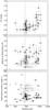 |
Fig. 6 Extinction and distance of 43 stars estimated using the method described in Sect. 4.1 (top panel). Degree of polarization (%) versus distance and position angle versus distance plots for these stars are shown in the middle and bottom panels, respectively. The broken line is drawn at a distance of 450 pc where the first abrupt rise in the value of extinction was seen. The open circles show the polarization results obtained from the Heiles (2000) catalog of stars selected from a region of 20°× 20° field containing Gal 110-13 and Gal 96-15 clouds. The distance to these stars are calculated using the new Hipparcos parallax measurements given by van Leeuwen (2007). |
Of the 207 stars for which we have polarization measurements, 43 of them were classified as main sequence stars using the method described above. These sources are those that satisfied the conditions of (J−Ks) ≤0.75 and photometric errors in JHKs≤ 0.03 magnitude. In Fig. 6, the upper panel shows the derived extinction as a function of their distance. The plot shows a rapid increase in the value of extinction close to a distance of 450 pc (broken line). This slightly disagrees with the distance obtained using extinction of stars from a larger area of Gal 110-13. In the middle and the lower panels, we present the variations in P% and θP as a function of distance. Normally, the degree of polarization, similar to the extinction due to the dust grains, rises with the increase in the column of dust grains along the pencil beam of a star. When the pencil beam of the star passes through a dust cloud, the P% tends to show a rapid increase in the value if there is no significant change in the direction of the alignment of the dust grains along the line-of-sight. Therefore by combining the polarization and distance information of stars projected on a cloud, the distance to the cloud can be estimated (e.g., Alves et al. 2008). The measured values of P% show an increase from ~0.5% to ~2% at around 450 pc similar to the rise seen in the extinction values. Because the values of P% shown in Fig. 6 are actual measurements, the rise observed in P% at around 450 pc seems to be more genuine. In that case, the presence of a number of stars with relatively high values of extinction at distances close to 350 pc seen in Fig. 4 could either be due to wrongly classifying of them as main sequence stars, or that there are additional dust components between Gal 110-13 and us. No further information such as parallax or spectral type is available for these sources in the literature. Employing the same method as used in this work, Soam et al. (2013) estimated a distance of 360 ± 65 pc to another cometary globule, Gal 96-15, located at 14° to the west of Gal 110-13. The absorbing material at around 350 pc is being consistently detected in the AV versus distance diagrams of both Gal 110-13 and Gal 96-15, suggesting that the presence of this absorbing layer could possibly be real.
To understand the global distribution of interstellar material toward the region containing Gal 110-13 and Gal 96-15, we searched for sources within a region with a 20°× 20° field that has both polarization and parallax measurements (Heiles (2000) and van Leeuwen (2007), respectively). The polarization results are shown in Fig. 6 (middle and lower panels) and polarization vectors are drawn in Fig. 11. The length and the orientation of the vectors drawn in Fig. 11 correspond to the P% and the position angle measured from the galactic north (increasing eastward), respectively. The P% values from the Heiles (2000) catalog show an increase at around 200 pc by ~0.5% and then a possible increase from ~0.5% to ~1% at around 320 pc giving evidence of at least two additional dust components lying toward the direction of Gal 110-13. It is quite intriguing that the P% values show a decreasing trend after 450 pc as against what is expected. The contributions from these foreground absorbing material could be the most likely cause of a few stars in Fig. 4 showing relatively high values of extinction at distances less than 450 pc (the distance at which the P% values show a sudden jump in Fig. 6).
The B-type star, HD 222142 that illuminates the reflection nebula vdB 158, is found to share a common proper motion with the Lac OB1 association (Lee & Chen 2007). This suggests that there could be a possible link between Gal 110-13 and the Lac OB1. The distance estimated to Lac OB1 (which includes the distance to the association as a whole and to the individual subgroups) ranges from ~350 pc to ~600 pc (Kaltcheva 2009). Using the available uvbyβ photometry of the stars earlier than A0 type from a 20° × 20° field (similar to what is considered by us to obtain polarimetric results from the Heiles (2000) catalog), Kaltcheva (2009) estimate an average distance of 520 ± 20 pc to a group of 12 stars that are often identified as members of the Lac OB 1 association. However, the photometric distance to the most massive member of Lac OB1 association, 10 Lac, is found to be 715 pc (Kaltcheva 2009). But the distance of 10 Lac estimated using new Hipparcos parallax from van Leeuwen (2007) puts the star at 529
 pc which is in good agreement with the average distance estimated for the Lac OB 1 association.
We note that given the galactic latitude of 10 Lac b = −16.98°, a distance of ~700 pc would place this star about 200 pc away from the galactic plane. This is about a factor of four higher than the typical scale height of star clusters of age ≲10 Myr (Reed 2000; Buckner & Froebrich 2014). The color excess versus distance plot presented by Kaltcheva (2009) clearly shows the presence of absorbing material even at ~150 pc, giving additional evidence that there is foreground absorbing material toward the direction of Gal 110-13. Based on optical photometry obtained using PanSTARRS-1, Schlafly et al. (2014) estimate a distance of 510 ± 51 pc to Gal 96-15. They also find evidence of material distributed at ~300 pc. In a more recent study based on non-LTE analysis of high quality data, Nieva & Przybilla (2014) estimate fundamental parameters of 26 early B-type stars in OB associations. Of these, they estimated a distance of 398 ± 26 pc to HD 216916 (also called EN Lac, B1.5IV) which is considered to be a member of the Lac OB1 association.
Although the distance to the Lac OB1 association, to 10 Lac and to the surrounding clouds is still uncertain, we assign 450 ± 80 pc as the most probable distance to Gal 110-13 based on the results obtained from our polarimetric measurements. The uncertainty in the distance estimated using the 2MASS photometry, described above, is found to be typically be about 18% (Maheswar et al. 2010). Additionally, one of the stars, HD 221515, located within an angular separation of ≲1° from Gal 110-13 and located at a distance of ~450 pc, is found to show polarization angle similar to the average value (45°) of the measured position angles of the stars projected on the cloud. This gives an additional reason to believe that Gal 110-13 is located roughly at or closer than ~450 pc.
4.2. The foreground interstellar polarization subtraction
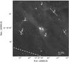 |
Fig. 7 Seven stars having parallax measurements by the Hipparcos satellite within a circular region of 2° diameter around Gal 110-13 are identified in the WISE 12 μm image. The polarization vectors are drawn so that the length corresponds to the degree of polarization, and the orientation corresponds to the position angle measured from the north toward the east. A 0.2% vector is drawn for reference. The broken line shows the orientation of the Galactic plane. Five of these seven stars are used to subtract the foreground interstellar polarization from the observed values. |
Polarization values of the seven foreground stars.
To remove the foreground interstellar polarization from the observed polarization values, we made a search around Gal 110-13 within a circular region of 2° diameter for stars having parallax measurements made by the Hipparcos satellite in van Leeuwen (2007). We excluded those that are identified as emission line sources, in binary or multiple systems or peculiar sources in the SIMBAD. Stars with the ratio of the parallax measurements and the error in parallax ≥2 were chosen. The distance of these stars range from ~90 to ~450 pc. We made polarization observations of these seven stars in the R-band using AIMPOL. In Table 3, we present the results ordered according to their increasing distance from the Sun. The positions of these stars with respect to Gal 110-13 are shown in the 2°×2° WISE 12 μm image in Fig. 7.
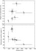 |
Fig. 8 Upper panel: degree of polarization versus distance of the seven stars found within 2° diameter of Gal 110-13. The distances are calculated from the Hipparcos parallax measurements taken from van Leeuwen (2007). Lower panel: polarization position angle versus distance for the same stars. The five stars lying foreground to Gal 110-13 are used to subtract the foreground interstellar polarization from the measured values. |
The P% and θP of the seven stars with their distances are shown in Fig. 8. We estimated the weighted mean of P% and θP using five of the seven stars. We excluded the source at ~90 pc because it shows almost zero polarization. We also excluded the source located at ~450 pc because the θP value of this source (42°) is similar to the mean value of the θP obtained for the sources projected on Gal 110-13. We suspect that this source lies either behind or very close to Gal 110-13. The weighted mean values of the degree of polarization and the position angles are found to be 0.3% and 73°.
Using these values, we calculated the mean Stokes parameters Qfg( = Pcos2θ) and Ufg( = Psin2θ) as −0.249 and 0.168, respectively. We also calculated the Stokes parameters Q⋆ and U⋆, for the target sources. Then we estimated the foreground-corrected Stokes parameters Qc and Uc of the target sources using Qc = Q⋆−Qfg and Uc = U⋆−Ufg. The corresponding foreground-corrected degree of polarization (Pc) and the position angle (θc) values of the target stars were estimated using the equations  and
and  . After the foreground subtraction, 186 target stars satisfied the condition of P/σP≥ 2. The polarization vectors of 186 foreground-subtracted stars are overplotted on the WISE 12 μm image as shown in Fig. 9. The IRAS 100 μm intensity contours are also overplotted. The length and the orientation of the vectors correspond to the measured P% and θP values, respectively. The θP is measured from the north increasing toward the east. A vector with 2% polarization is shown for reference as is the orientation of the Galactic plane at the galactic latitude of −13°.
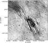 |
Fig. 9 Polarization vectors are over plotted on the WISE 12 μm image of Gal 110-13. The IRAS 100μm contours are also overlayed on the image. The contours start from 6.0 MJy/sr to 31.2 MJy/sr in increments of 2.8 MJy/sr. The length of the vectors corresponds to the degree of polarization, and orientation corresponds to the position angle measured from the north and increasing toward the east. A vector corresponding to 2% polarization is shown for reference. The dashed line in white shows the orientation of the Galactic plane. |
4.3. The cause of the unusual structure of the cloud
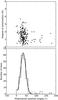 |
Fig. 10 Degree of polarization versus the polarization position angle of stars projected on Gal 110-13. The histogram of the position angles is also presented. These values are obtained after subtracting the foreground interstellar component from the observed values. The solid curve represents a fit to the histogram of position angles. |
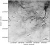 |
Fig. 11 Region containing Gal 96-15, Gal 110-13, and 10 Lac are shown in the IRAS 100 μm image. The ambient magnetic field direction at the location of Gal 96-15 is drawn. The mean magnetic field direction corrected for the foreground interstellar contribution is drawn at the position of Gal 110-13. The arrows show the direction of propagation of ionizing radiation from 10 Lac toward Gal 96-15 and Gal 110-13. The vectors drawn in black are based on the polarization results obtained from the Heiles (2000) catalog. The length and the orientation of the vectors correspond to the degree of polarization and the position angles measured from the galactic north increasing to the east. A vector corresponding to 1% polarization is shown for reference. |
The mean values of P% after the removal of the foreground interstellar polarization is obtained as 1.5%. The mean value of θP from a Gaussian fit to the data is found to be 40° which is considered as the mean direction of the plane of the sky component of magnetic field in Gal 110-13. The plot of P% vs. θP and the histogram of the θP after correcting for the foreground interstellar contribution are shown in Fig. 10. The standard deviation of θP values is found to be ~11° implying that the magnetic field lines in Gal 110-13 are ordered relatively well.
Based on far-infrared, HI, and CO data of the region, Odenwald et al. (1992) proposed cloud-cloud collision scenario as the most preferred mechanism responsible for the formation of Gal 110-13. They suggested that the Gal 110-13 was formed as a result of the interaction between two HI clouds moving across the line of sight and having velocity components of −8 and −6 km s-1. They also suggested that the southern part compared to the northern part is in an advanced stage that resulted in it being predominantly molecular. Head-on supersonic collision between two identical magnetized clouds was studied using 3D-SPMHD simulations under two special cases of parallel and perpendicular magnetic field orientations with respect to the motion of the colliding clouds (Marinho et al. 2001). The magnetic field was amplified and deformed in the shocked layers in both those cases. In the perpendicular magnetic field configuration, owing to the interaction of the clouds, field lines are compressed in the shocked layer forming a magnetic shield that acts like an elastic bumper between the clouds. This prevents the direct contact of the clouds and also their disruption during the interaction (Jones et al. 1996).
Formation of clumps was noticed only in the case of parallel field configuration. Because star formation is active in Gal 110-13 (Aveni & Hunter 1969; Odenwald et al. 1992), and if the cloud was formed as a result of cloud-cloud collision, the initial field configuration would have been parallel to the cloud motion. According to HI observations by Odenwald et al. (1992), collided clouds have traveled across the line of sight in the northeast-southwest direction. But the current magnetic field geometry is almost perpendicular to the proposed direction of the interaction of the clouds. Also, the simulations show that in both parallel and perpendicular cases the field distribution after the shock interaction was found to be chaotic especially on the large scales, irrespective of the initial field configuration (Marinho et al. 2001). However, the observed magnetic field lines from polarization are found to be uniformly distributed in contrast to the results from the simulations.
Lee & Chen (2007) have considered either a supernova explosion or ionization fronts from a massive star in the vicinity of Gal 110-13 as an alternate mechanism that might have caused its cometary shape. In a supernova scenario, a massive star, which is probably a member of Lac OB1 association to which 10 Lac is considered to be a member, could have exploded as a supernova. The shock waves from such an explosion could have traveled to the location of Gal 110-13 at a speed of hundreds of km s-1 to reach Gal 110-13 and compress the cloud to give its present shape and trigger the star formation. In an ionization-front-induced formation scenario of Gal 110-13, the ionizing photons from 10 Lac, soon after its birth, might have compressed the cloud, creating a cometary morphology and subsequent star formation (Lee & Chen 2007). The spatial separation between Gal 110-13 and 10 Lac is estimated to be ~110 pc by adopting a distance of 450 pc to Gal 110-13. However, if we consider the most distant distance of 715 pc to 10 Lac estimated by Kaltcheva (2009), and assume that Gal 110-13 also lies at the same distance, then the spatial separation between 10 Lac and Gal 110-13 becomes ~180 pc. As pointed out by Lee & Chen (2007), the ionization front would take about ~2–3 Myr time to travel the distance of ~110–180 pc between 10 Lac and Gal 110-13. This is relatively shorter than the 5.5 ± 0.5 Myr age estimated for 10 Lac by Tetzlaff et al. (2011).
Based on the radiation-magnetohydrodynamics (R-MHD) simulations of globules (Henney et al. 2009; Mackey & Lim 2011), it was shown that both radiation-driven implosion and acceleration of clumps by the rocket effect2 tend to align the magnetic field with the direction of propagation of ionizing photons in the globules. The efficiency of this alignment depends on the initial magnetic field strength. While the field reorientation is prevented significantly in a strong magnetic field scenario (~150–180 μG), in the case of medium and weak (~50 μG) field strengths, the field lines are dragged into alignment with the direction of the ionizing radiation. The structure of a dynamically evolving globule subjected to photo-ionization depends on the initial magnetic field orientation. Simulations with three initial field orientations (perpendicular, parallel, and inclined) with respect to the direction of propagation of the photo-ionizing radiation have been carried out by Henney et al. (2009). In the case of strong perpendicular initial magnetic field, the globule evolution is found to be highly anisotropic. The globule becomes flattened in the direction of magnetic field lines. But in the case of strong or weak parallel initial magnetic field, the globule remains cylindrically symmetric throughout its evolution. Also, since the magnetic field opposes the lateral compression of the neutral globule, it becomes broader with a snubber head.
The magnetic field strength estimated in Gal 110-13 is found to be ~25 μG (section 4.4) assuming the distance as 450 pc. The region containing Gal 110-13, Gal 96-15 and 10 Lac is shown in Fig. 11. It is interesting to note that the elongated structure of Gal 110-13 is aligned roughly to the line joining the cloud and the 10 Lac which is ~70° with respect to the galactic north (also considered as the direction of propagation of the ionizing photons from 10 Lac). In Fig. 11, we also show the mean value of the magnetic field direction in Gal 110-13 drawn at an angle of ~60° with respect to the galactic north. The mean value of the polarization position angles, obtained from the Heiles (2000) catalog, of the stars located within the 20° × 20° field (as shown in Fig. 11) is found to be ~100° with respect to the galactic north. This is considered to be the direction of the initial magnetic field prior to the ionization of the region by the 10 Lac.
The magnetic field geometry of Gal 96-15 was mapped by Soam et al. (2013). The initial magnetic field orientation toward Gal 96-15 prior to the cloud being hit by the ionizing radiation from the 10 Lac was inferred as ~95° (Soam et al. 2013) with respect to the galactic north. This is consistent with the direction of the initial field direction inferred using a larger sample of stars distributed over a wider area in this study. Thus the initial magnetic field direction is offset by ~30° with respect to the line joining the cloud and 10 Lac. The ionizing photons from 10 Lac might have reoriented the relatively weak ~25 μG magnetic field and made it aligned with the direction of propagation, thus creating the unusually long cometary shape of the cloud. On the other hand the line joining the head part of Gal 96-15 and 10 Lac makes an angle of ~1° with respect to the galactic north (see Fig. 11). The initial magnetic field in Gal 96-15 was therefore oriented almost perpendicular to the direction of propagation of the ionizing photons from the 10 Lac. Accordingly, Gal 110-13 and Gal 96-15 could be considered as good examples of the photo-ionization of clouds with the magnetic field oriented parallel and perpendicular to the direction of propagation of the ionizing radiation, respectively. As also seen in simulations, the difference in the orientation of magnetic field direction with respect to the direction of the propagation of the ionizing photons could be the reason for the difference in the physical structure of both the clouds. While Gal 110-13 shows an elongated cloud structure with ~1° in extent, Gal 96-15 shows a comma structure with the tail part curled almost perpendicular to the line joining the cloud and the 10 Lac and almost aligning with the inferred initial magnetic field direction. This suggests that the magnetic field in Gal 96-15 might be stronger than the field strength estimated in Gal 110-13, causing the field to resist its reorientation along the direction of 10 Lac.
4.4. The structure function
The strength of the magnetic field can be estimated by determining the turbulent angular dispersion in Gal 110-13. Hildebrand et al. (2009) assumed that the net magnetic field is basically a combination of large-scale structured field, B0(x), and a turbulent component, Bt(x). Initially in this method the angular dispersion function (ADF) or the square root of the structure function is calculated, which is defined as the root mean-squared differences between the polarization angles measured for all pairs of points (N(l)) separated by a distance l (see Eq. (3)). The ADF shows the dispersion of the polarization angles as a function of the distance in a specific region.
Recently, this method has been used as an important statistical tool to infer the relationship between the large-scale structured field and the turbulent component of the magnetic field in molecular clouds (e.g., Hildebrand et al. 2009; Franco et al. 2010; Santos et al. 2012; Eswaraiah et al. 2013). The expression for the ADF is ![Mathematical equation: \begin{equation} \langle\Delta\phi^{2}(l)\rangle^{1/2} =\Bigg \{\frac{1}{N(l)} \sum\limits_{i = 1}^{N(l)} [\phi(x) - \phi(x+l)]^{2} \Bigg \}^{1/2} \end{equation}](/articles/aa/full_html/2016/04/aa26845-15/aa26845-15-eq137.png) (3)The total measured structure function within the range δ<l ≪ d, (where δ and d are the correlation lengths which characterize Bt(x) and B0(x), respectively), can be estimated using (Hildebrand et al. 2009):
(3)The total measured structure function within the range δ<l ≪ d, (where δ and d are the correlation lengths which characterize Bt(x) and B0(x), respectively), can be estimated using (Hildebrand et al. 2009): 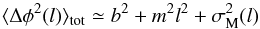 (4)where ⟨ Δφ2(l) ⟩ tot is the total measured dispersion estimated from the data. The quantity
  is the measurement uncertainties, which are calculated by taking the mean of the variances on Δφ(l) in each bin. The quantity b2 is the constant turbulent contribution, estimated by the intercept of the fit to the data after subtracting . The quantity m2l2 is a smoothly increasing contribution with the length l (m shows the slope of this linear behavior). All these quantities are statistically independent of each other.
The ratio of the turbulent component and the large-scale magnetic fields is given by the equation:  (5)For the Gal 110-13 region we estimated the ADF and plotted it with the distance in the Fig. 12. We used the polarization angle of 169 stars to calculate ADF. The measured errors in each bin are very small, which are also overplotted in the Fig. 12. Each bin denotes the
  which is the ADF corrected for the measurement uncertainties. Bin widths are taken on logarithmic scale. We used only five points of the ADF in the linear fit of Eq. (4). The shortest distance we considered is ≃0.1 pc. The net turbulent contribution to the angular dispersion, b, is calculated to be 9.5° ± 0.2° (0.17 ± 0.003 rad). Then we estimated the ratio of the turbulent component and the large-scale magnetic fields using Eq. (5), which is found to be 0.12 ± 0.002. The result shows that the turbulent component of magnetic field is very small in comparison to the large-scale structured magnetic field, i.e., Bt ≪ B0.
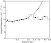 |
Fig. 12 Angular dispersion function (ADF) of the polarization angles, ⟨ Δφ2(l) ⟩ 1/2 (°), with distance (pc) for 169 stars of Gal 110-13. The dashed line denotes the best fit to the data up to ~1 pc distance. |
The strength of the plane of the sky component of the magnetic field was estimated using the expression (Franco & Alves 2015), ![Mathematical equation: \begin{equation} B_\mathrm{pos} = 9.3 \left[\frac{2~n_{\rm H_{2}}}{\rm cm^{-3}} \right]^{1/2} \left[\frac{\Delta V}{\rm km \,s^{-1}} \right] \left[\frac{b}{1^{\circ}} \right]^{-1}~~\mu {\rm G} \label{equ:B_field} \end{equation}](/articles/aa/full_html/2016/04/aa26845-15/aa26845-15-eq157.png) (6)in which the scale factor Q ≈ 0.5 is considered based on the results obtained from numerical studies (e.g., Ostriker et al. 2001). The above expression was derived by modifying the classical method proposed by Chandrasekhar & Fermi (1953) where they suggested that the analysis of the small-scale randomness of magnetic field could be used to estimate the field strength. This method relates the line-of-sight velocity dispersion to the irregular scatter in the polarization position angles under the assumptions that there is a mean field component in the area of interest, that the turbulence responsible for the magnetic field perturbations is isotopic, and that there is equipartition between the turbulent kinetic and magnetic energy (Heitsch et al. 2001). The volume number density of molecular hydrogen is obtained by estimating the column density of the region probed by our optical polarimetry and from the thickness of the cloud, assuming it to be a cylindrical filament. We used the relation, N(H2)/Av = 9.4 × 1020 cm-2 mag-1 (Bohlin et al. 1978) for obtaining the column density. Based on the method described in 4.1, the average value of extinction traced by the stars lying behind the cloud (distance ≳450 pc) observed in this study is found to be ~0.6 mag (see Fig. 6). The angular diameter of the cloud is found to be ~8′. Considering 450 pc as the distance to Gal 110-13, the value of n(H2) is found to be ~175 cm-3. However, if we consider the farthest distance of 10 Lac estimated by Kaltcheva (2009) as the distance to Gal 110-13 also, then the value of n(H2) becomes ~110 cm-3. We obtained the 12CO line width (ΔV = 1.4 km s-1) toward Gal 110-13 from Odenwald et al. (1992). The turbulent contribution to the angular dispersion is found to be b = 9.5° ± 0.2°. Substituting these values in Eq. (6), we obtained Bpos as ~25 μG for a distance of 450 pc and ~20 μG if the distance is taken as 715 pc. The obtained values of Bpos should be considered as a rough estimate only mainly due to the large uncertainties involved in the quantities used in their calculations. Apart from the uncertainties in the measurement of line width and in the estimation of b parameter, the dominant source of uncertainty in the above calculation of Bpos is in the determination of the molecular hydrogen density.
(6)in which the scale factor Q ≈ 0.5 is considered based on the results obtained from numerical studies (e.g., Ostriker et al. 2001). The above expression was derived by modifying the classical method proposed by Chandrasekhar & Fermi (1953) where they suggested that the analysis of the small-scale randomness of magnetic field could be used to estimate the field strength. This method relates the line-of-sight velocity dispersion to the irregular scatter in the polarization position angles under the assumptions that there is a mean field component in the area of interest, that the turbulence responsible for the magnetic field perturbations is isotopic, and that there is equipartition between the turbulent kinetic and magnetic energy (Heitsch et al. 2001). The volume number density of molecular hydrogen is obtained by estimating the column density of the region probed by our optical polarimetry and from the thickness of the cloud, assuming it to be a cylindrical filament. We used the relation, N(H2)/Av = 9.4 × 1020 cm-2 mag-1 (Bohlin et al. 1978) for obtaining the column density. Based on the method described in 4.1, the average value of extinction traced by the stars lying behind the cloud (distance ≳450 pc) observed in this study is found to be ~0.6 mag (see Fig. 6). The angular diameter of the cloud is found to be ~8′. Considering 450 pc as the distance to Gal 110-13, the value of n(H2) is found to be ~175 cm-3. However, if we consider the farthest distance of 10 Lac estimated by Kaltcheva (2009) as the distance to Gal 110-13 also, then the value of n(H2) becomes ~110 cm-3. We obtained the 12CO line width (ΔV = 1.4 km s-1) toward Gal 110-13 from Odenwald et al. (1992). The turbulent contribution to the angular dispersion is found to be b = 9.5° ± 0.2°. Substituting these values in Eq. (6), we obtained Bpos as ~25 μG for a distance of 450 pc and ~20 μG if the distance is taken as 715 pc. The obtained values of Bpos should be considered as a rough estimate only mainly due to the large uncertainties involved in the quantities used in their calculations. Apart from the uncertainties in the measurement of line width and in the estimation of b parameter, the dominant source of uncertainty in the above calculation of Bpos is in the determination of the molecular hydrogen density.
4.5. The polarization efficiency
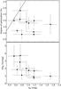 |
Fig. 13 Upper panel: P% versus AR plot of stars for which AR/σAR≥ 2. The solid line represents the observational upper limit of the polarization efficiency. Lower panel: P/AR versus AR plot. |
The ratio of the degree of polarization to extinction is a measure of the efficiency of polarization produced by the interstellar medium. The efficiency depends on the nature of dust grains and the efficiency with which the dust grains are aligned with the local magnetic field along the line of sight. A theoretical upper limit on the polarization efficiency was calculated by assuming dust grains of infinite cylinders with diameter comparable to the wavelength and the long axes aligned perfectly parallel to one another.
We determined AV values for 43 stars toward Gal 110-13 using the method mentioned in 4.1. In Fig. 13 (upper panel), we show the PR as a function of AR values obtained using AR/AV = 0.748 (Rieke & Lebofsky 1985). The 11 stars are plotted with the condition AV/σ(AV) ≥ 2. The solid line is drawn for the observational upper limit evaluated for the λeff = 0.760 μm. The relation between PV and PR is obtained using the empirical formula given by Serkowski et al. (1975). Here we used the typical values of the parameter K = −1.15, which determines the width of the peak of the curve, and λmax = 0.55 μm for the calculations, which may depend on observer’s line of sight (Whittet 1992). The transformed observational upper limit is found to be PR/AR ≈ 4% /mag. Toward Gal 110-13 region, the polarizing efficiency of dust grains are found to be below the observational limit. In Fig. 13 (lower panel), we present polarization efficiency as a function of extinction. The data are consistent with a trend toward very rapidly decreasing PR/AR with the extinction. The polarizing efficiency tends to be higher for stars with low extinction and becomes lower for those with high values of extinction. Thus the population of dust polarizing the background starlight are dominated by those lying in the outer layers of the cloud and the field orientation probed using optical polarization are predominantly of the one on the periphery of the clouds.
5. Conclusions
We present R-band polarization measurements of 207 stars projected on an unusual, cometary shaped cloud, Gal 110-13. The main goal of the study was to identify the most likely mechanism responsible for its cometary structure and ongoing star formation activity in the cloud. Based on the results from our polarization measurements of stars projected on the cloud and evaluating their distances using 2MASS photometry, we estimated a distance of 450 ± 80 pc to Gal 110-13. The foreground interstellar polarization component was removed from the observed polarization measurements by observing a number of stars located within a circular region of 2° diameter and having parallax measurements made by the Hipparcos satellite. The magnetic field thus inferred from the foreground corrected polarization values are found to be parallel to the elongated structure of the cloud. The field lines are found to be distributed uniformly over the cloud. The plane of the sky magnetic field strength estimated using the structure function analysis was found to be ~25 μG. Based on our polarimetric results, we suggest that the compression of the cloud by the ionization fronts from 10 Lac is the most likely mechanism responsible for creating the cometary shape and the star formation activity in Gal 110-13.
The loci of main sequence stars and the classical T-Tauri stars (CTTS, Meyer et al. 1997) intercept at (J−Ks) ≈0.75. Therefore the condition (J−Ks) ≤0.75 allows us to exclude both stars later than K7V and CTTS from the analysis.
Acceleration of the globule away from the ionizing source, caused due to the back reaction of the transonic photo-evaporation flow that leaves the ionization front and moves toward the ionizing source.
Acknowledgments
The authors are very grateful to the referee, Prof. Gabriel Franco, for the constructive comments and suggestions, that helped considerably to improve the content of the manuscript. This research made use of the SIMBAD database, operated at the CDS, Strasbourg, France. We also acknowledge the use of NASA’s SkyView facility (http://skyview.gsfc.nasa.gov) located at NASA Goddard Space Flight Center. This research also made use of APLpy, an open-source plotting package for Python hosted at http://aplpy.github.com. C.W.L was supported by Basic Science Research Program though the National Research Foundation of Korea (NRF) funded by the Ministry of Education, Science, and Technology (NRF-2013R1A1A2A10005125) and also by the global research collaboration of Korea Research Council of Fundamental Science & Technology (KRCF). S.N. thanks Suvendu Rakshit (OCA, Nice) for his valuable support and useful discussions.
References
- Alves, F. O., Franco, G. A. P., & Girart, J. M. 2008, A&A, 486, L13 [NASA ADS] [CrossRef] [EDP Sciences] [Google Scholar]
- Alves, F. O., Frau, P., Girart, J. M., et al. 2014, A&A, 569, L1 [NASA ADS] [CrossRef] [EDP Sciences] [Google Scholar]
- Anathpindika, S. 2009, A&A, 504, 437 [NASA ADS] [CrossRef] [EDP Sciences] [Google Scholar]
- Anathpindika, S. V. 2010, MNRAS, 405, 1431 [NASA ADS] [Google Scholar]
- Aveni, A. F., & Hunter, Jr., J. H. 1969, AJ, 74, 1021 [NASA ADS] [CrossRef] [Google Scholar]
- Bahcall, J. N., & Soneira, R. M. 1980, ApJS, 44, 73 [NASA ADS] [CrossRef] [Google Scholar]
- Bertoldi, F. 1989, ApJ, 346, 735 [NASA ADS] [CrossRef] [Google Scholar]
- Bertoldi, F., & McKee, C. F. 1990, ApJ, 354, 529 [NASA ADS] [CrossRef] [Google Scholar]
- Bertrang, G., Wolf, S., & Das, H. S. 2014, A&A, 565, A94 [NASA ADS] [CrossRef] [EDP Sciences] [Google Scholar]
- Bhatt, H. C. 1999, MNRAS, 308, 40 [NASA ADS] [CrossRef] [Google Scholar]
- Bhatt, H. C., Maheswar, G., & Manoj, P. 2004, MNRAS, 348, 83 [NASA ADS] [CrossRef] [Google Scholar]
- Bohlin, R. C., Savage, B. D., & Drake, J. F. 1978, ApJ, 224, 132 [NASA ADS] [CrossRef] [Google Scholar]
- Brand, P. W. J. L., Hawarden, T. G., Longmore, A. J., Williams, P. M., & Caldwell, J. A. R. 1983, MNRAS, 203, 215 [NASA ADS] [Google Scholar]
- Buckner, A. S. M., & Froebrich, D. 2014, MNRAS, 444, 290 [NASA ADS] [CrossRef] [Google Scholar]
- Cappa de Nicolau, C., & Olano, C. A. 1990, Rev. Mex. Astron. Astrofis., 21, 269 [NASA ADS] [Google Scholar]
- Cashman, L. R., & Clemens, D. P. 2014, ApJ, 793, 126 [NASA ADS] [CrossRef] [Google Scholar]
- Chandrasekhar, S., & Fermi, E. 1953, ApJ, 118, 113 [NASA ADS] [CrossRef] [Google Scholar]
- Chapman, N. L., Goldsmith, P. F., Pineda, J. L., et al. 2011, ApJ, 741, 21 [NASA ADS] [CrossRef] [Google Scholar]
- Clemens, D. P. 2012, ApJ, 748, 18 [NASA ADS] [CrossRef] [Google Scholar]
- Clemens, D. P., & Barvainis, R. 1988, ApJS, 68, 257 [NASA ADS] [CrossRef] [Google Scholar]
- Cutri, R. M., Skrutskie, M. F., van Dyk, S., et al. 2003, VizieR Online Data Catalog: II/246 [Google Scholar]
- Davis, Jr., L., & Greenstein, J. L. 1951, ApJ, 114, 206 [Google Scholar]
- Dotson, J. L., Davidson, J., Dowell, C. D., Schleuning, D. A., & Hildebrand, R. H. 2000, ApJS, 128, 335 [NASA ADS] [CrossRef] [Google Scholar]
- Dotson, J. L., Vaillancourt, J. E., Kirby, L., et al. 2010, ApJS, 186, 406 [NASA ADS] [CrossRef] [Google Scholar]
- Eswaraiah, C., Maheswar, G., Pandey, A. K., et al. 2013, A&A, 556, A65 [NASA ADS] [CrossRef] [EDP Sciences] [Google Scholar]
- Franco, G. A. P., & Alves, F. O. 2015, ApJ, 807, 5 [NASA ADS] [CrossRef] [Google Scholar]
- Franco, G. A. P., Alves, F. O., & Girart, J. M. 2010, ApJ, 723, 146 [Google Scholar]
- Gilden, D. L. 1984, ApJ, 279, 335 [NASA ADS] [CrossRef] [Google Scholar]
- Goodman, A. A. 1996, in Polarimetry of the Interstellar Medium, eds. W. G. Roberge, & D. C. B. Whittet, ASP Conf. Ser., 97, 325 [Google Scholar]
- Goodman, A. A., Bastien, P., Menard, F., & Myers, P. C. 1990, ApJ, 359, 363 [NASA ADS] [CrossRef] [Google Scholar]
- Goodman, A. A., Jones, T. J., Lada, E. A., & Myers, P. C. 1995, ApJ, 448, 748 [NASA ADS] [CrossRef] [Google Scholar]
- Grinin, V. P., Kolotilov, E. A., & Rostopchina, A. 1995, A&AS, 112, 457 [NASA ADS] [Google Scholar]
- Gritschneder, M., Burkert, A., Naab, T., & Walch, S. 2010, ApJ, 723, 971 [NASA ADS] [CrossRef] [Google Scholar]
- Habe, A., & Ohta, K. 1992, PASJ, 44, 203 [NASA ADS] [Google Scholar]
- Hausman, M. A. 1981, ApJ, 245, 72 [NASA ADS] [CrossRef] [Google Scholar]
- Heiles, C. 2000, AJ, 119, 923 [NASA ADS] [CrossRef] [Google Scholar]
- Heitsch, F., Zweibel, E. G., Mac Low, M.-M., Li, P., & Norman, M. L. 2001, ApJ, 561, 800 [NASA ADS] [CrossRef] [Google Scholar]
- Henney, W. J., Arthur, S. J., de Colle, F., & Mellema, G. 2009, MNRAS, 398, 157 [NASA ADS] [CrossRef] [Google Scholar]
- Herbig, G. H., & Bell, K. R. 1988, Third Catalog of Emission-Line Stars of the Orion Population (Santa Cruz: University of California, Lick Observatory) [Google Scholar]
- Hildebrand, R. H. 1988, QJRAS, 29, 327 [NASA ADS] [Google Scholar]
- Hildebrand, R. H., Kirby, L., Dotson, J. L., Houde, M., & Vaillancourt, J. E. 2009, ApJ, 696, 567 [NASA ADS] [CrossRef] [Google Scholar]
- Hiltner, W. A. 1949, Nature, 163, 283 [NASA ADS] [CrossRef] [Google Scholar]
- Hiltner, W. A. 1951, ApJ, 114, 241 [NASA ADS] [CrossRef] [Google Scholar]
- Hoang, T., & Lazarian, A. 2014, MNRAS, 438, 680 [NASA ADS] [CrossRef] [Google Scholar]
- Hull, C. L. H., Plambeck, R. L., Kwon, W., et al. 2014, ApJS, 213, 13 [NASA ADS] [CrossRef] [Google Scholar]
- Jones, T. W., Ryu, D., & Tregillis, I. L. 1996, ApJ, 473, 365 [NASA ADS] [CrossRef] [Google Scholar]
- Kaltcheva, N. 2009, PASP, 121, 1045 [NASA ADS] [CrossRef] [Google Scholar]
- Kessel-Deynet, O., & Burkert, A. 2003, MNRAS, 338, 545 [NASA ADS] [CrossRef] [Google Scholar]
- Keto, E. R., & Lattanzio, J. C. 1989, ApJ, 346, 184 [NASA ADS] [CrossRef] [Google Scholar]
- Kimura, T., & Tosa, M. 1996, A&A, 308, 979 [NASA ADS] [Google Scholar]
- Klein, R. I., & Woods, D. T. 1998, ApJ, 497, 777 [NASA ADS] [CrossRef] [Google Scholar]
- Kusune, T., Sugitani, K., Miao, J., et al. 2015, ApJ, 798, 60 [NASA ADS] [CrossRef] [Google Scholar]
- Lattanzio, J. C., Monaghan, J. J., Pongracic, H., & Schwarz, M. P. 1985, MNRAS, 215, 125 [NASA ADS] [CrossRef] [Google Scholar]
- Lazarian, A. 2007, J. Quant. Spec. Radiat. Transf., 106, 225 [NASA ADS] [CrossRef] [Google Scholar]
- Lee, H.-T., & Chen, W. P. 2007, ApJ, 657, 884 [NASA ADS] [CrossRef] [Google Scholar]
- Lefloch, B., & Lazareff, B. 1994, A&A, 289, 559 [NASA ADS] [Google Scholar]
- Lefloch, B., & Lazareff, B. 1995, A&A, 301, 522 [Google Scholar]
- Mackey, J., & Lim, A. J. 2010, MNRAS, 403, 714 [NASA ADS] [CrossRef] [Google Scholar]
- Mackey, J., & Lim, A. J. 2011, MNRAS, 412, 2079 [NASA ADS] [CrossRef] [Google Scholar]
- Maheswar, G., Lee, C. W., Bhatt, H. C., Mallik, S. V., & Dib, S. 2010, A&A, 509, A44 [NASA ADS] [CrossRef] [EDP Sciences] [Google Scholar]
- Maheswar, G., Lee, C. W., & Dib, S. 2011, A&A, 536, A99 [NASA ADS] [CrossRef] [EDP Sciences] [Google Scholar]
- Meyer, M. R., Calvet, N., & Hillenbrand, L. A. 1997, AJ, 114, 288 [NASA ADS] [CrossRef] [Google Scholar]
- Marinho, E. P., & Lépine, J. R. D. 2000, A&AS, 142, 165 [NASA ADS] [CrossRef] [EDP Sciences] [Google Scholar]
- Marinho, E. P., Andreazza, C. M., & Lépine, J. R. D. 2001, A&A, 379, 1123 [NASA ADS] [CrossRef] [EDP Sciences] [Google Scholar]
- Miao, J., White, G. J., Thompson, M. A., & Nelson, R. P. 2009, ApJ, 692, 382 [NASA ADS] [CrossRef] [Google Scholar]
- Miniati, F., Jones, T. W., Ferrara, A., & Ryu, D. 1997, ApJ, 491, 216 [NASA ADS] [CrossRef] [Google Scholar]
- Mizuta, A., Kane, J. O., Pound, M. W., et al. 2005, ApJ, 621, 803 [NASA ADS] [CrossRef] [Google Scholar]
- Nieva, M.-F., & Przybilla, N. 2014, A&A, 566, A7 [NASA ADS] [CrossRef] [EDP Sciences] [Google Scholar]
- Odenwald, S. F., & Rickard, L. J. 1987, ApJ, 318, 702 [NASA ADS] [CrossRef] [Google Scholar]
- Odenwald, S., Fischer, J., Lockman, F. J., & Stemwedel, S. 1992, ApJ, 397, 174 [NASA ADS] [CrossRef] [Google Scholar]
- Ostriker, E. C., Stone, J. M., & Gammie, C. F. 2001, ApJ, 546, 980 [NASA ADS] [CrossRef] [Google Scholar]
- Ramaprakash, A. N., Gupta, R., Sen, A. K., & Tandon, S. N. 1998, A&AS, 128, 369 [NASA ADS] [CrossRef] [EDP Sciences] [Google Scholar]
- Rao, R., Crutcher, R. M., Plambeck, R. L., & Wright, M. C. H. 1998, ApJ, 502, L75 [NASA ADS] [CrossRef] [Google Scholar]
- Rautela, B. S., Joshi, G. C., & Pandey, J. C. 2004, BASI, 32, 159 [NASA ADS] [Google Scholar]
- Reed, B. C. 2000, AJ, 120, 314 [NASA ADS] [CrossRef] [Google Scholar]
- Reipurth, B. 1983, A&A, 117, 183 [NASA ADS] [Google Scholar]
- Ricotti, M., Ferrara, A., & Miniati, F. 1997, ApJ, 485, 254 [NASA ADS] [CrossRef] [Google Scholar]
- Rieke, G. H., & Lebofsky, M. J. 1985, ApJ, 288, 618 [NASA ADS] [CrossRef] [Google Scholar]
- Sandford, S. A., Allamandola, L. J., Tielens, A. G. G. M., et al. 1992, in Astrochemistry of Cosmic Phenomena, ed. P. D. Singh, IAU Symp., 150, 133 [Google Scholar]
- Santos, F. P., Roman-Lopes, A., & Franco, G. A. P. 2012, ApJ, 751, 138 [NASA ADS] [CrossRef] [Google Scholar]
- Schlafly, E. F., Green, G., Finkbeiner, D. P., et al. 2014, ApJ, 786, 29 [NASA ADS] [CrossRef] [Google Scholar]
- Schmidt, G. D., Elston, R., & Lupie, O. L. 1992, AJ, 104, 1563 [NASA ADS] [CrossRef] [Google Scholar]
- Serkowski, K., Mathewson, D. S., & Ford, V. L. 1975, ApJ, 196, 261 [NASA ADS] [CrossRef] [Google Scholar]
- Soam, A., Maheswar, G., Bhatt, H. C., Lee, C. W., & Ramaprakash, A. N. 2013, MNRAS, 432, 1502 [NASA ADS] [CrossRef] [EDP Sciences] [Google Scholar]
- Sridharan, T. K., Bhatt, H. C., & Rajagopal, J. 1996, MNRAS, 279, 1191 [NASA ADS] [CrossRef] [Google Scholar]
- Stone, M. E. 1970a, ApJ, 159, 277 [NASA ADS] [CrossRef] [Google Scholar]
- Stone, M. E. 1970b, ApJ, 159, 293 [NASA ADS] [CrossRef] [Google Scholar]
- Sugitani, K., Nakamura, F., Watanabe, M., et al. 2011, ApJ, 734, 63 [Google Scholar]
- Takahira, K., Tasker, E. J., & Habe, A. 2014, ApJ, 792, 63 [NASA ADS] [CrossRef] [Google Scholar]
- Targon, C. G., Rodrigues, C. V., Cerqueira, A. H., & Hickel, G. R. 2011, ApJ, 743, 54 [NASA ADS] [CrossRef] [Google Scholar]
- Tetzlaff, N., Neuhäuser, R., & Hohle, M. M. 2011, MNRAS, 410, 190 [NASA ADS] [CrossRef] [Google Scholar]
- Tremblin, P., Audit, E., Minier, V., Schmidt, W., & Schneider, N. 2012, A&A, 546, A33 [NASA ADS] [CrossRef] [EDP Sciences] [Google Scholar]
- Vaillancourt, J. E., & Matthews, B. C. 2012, ApJS, 201, 13 [NASA ADS] [CrossRef] [Google Scholar]
- van Leeuwen, F. 2007, A&A, 474, 653 [NASA ADS] [CrossRef] [EDP Sciences] [Google Scholar]
- Vrba, F. J., Strom, S. E., & Strom, K. M. 1976, AJ, 81, 958 [NASA ADS] [CrossRef] [Google Scholar]
- Whitney, B. S. 1949, ApJ, 109, 540 [NASA ADS] [CrossRef] [Google Scholar]
- Whittet, D. C. B. 1992, Dust in the galactic environment (Taylor and Francis) [Google Scholar]
- Williams, R. J. R., Ward-Thompson, D., & Whitworth, A. P. 2001, MNRAS, 327, 788 [NASA ADS] [CrossRef] [Google Scholar]
Appendix A: Additional table
Polarization results of 207 stars (with P/σP≥ 2) observed in the direction of Gal 110-13.
All Tables
Polarization results of 207 stars (with P/σP≥ 2) observed in the direction of Gal 110-13.
All Figures
|
Fig. 1 Comparison of the degree of polarization (upper panel) and the position angles (lower panel) of the seven stars found in common with those observed by Grinin et al. (1995). |
| In the text | |
|
Fig. 2 (J−H) vs. (H−Ks) CC diagram drawn for stars (with AV ≥ 1) from the region containing Gal 110-13 to illustrate the method. The solid curve represents locations of unreddened main sequence stars. The reddening vector for an A0V type star drawn parallel to the Rieke & Lebofsky (1985) interstellar reddening vector is shown by the dashed line. The locations of the main sequence stars of different spectral types are marked with square symbols. The region to the right of the reddening vector is known as the near infrared excess region and corresponds to the location of pre-main sequence sources. The dash-dot-dash line represents the loci of unreddened CTTSs (Meyer et al. 1997). The open circles represent the observed colours, and the arrows are drawn from the observed to the final colours obtained by the method for each star. |
| In the text | |
|
Fig. 3 2° × 2° Planck 857 GHz image of Gal 110-13. The circles represent the positions of those sources that are plotted (closed circles) in the AV vs. distance plot (Fig. 4). |
| In the text | |
|
Fig. 4 AV vs. distance plot for the regions containing Gal 110-13 (closed circles) and CB 248 (open circles). The dashed vertical line is drawn at 345 pc inferred from the procedure described in Maheswar et al. (2010). The dash-dotted curve represents the increase in the extinction towards the Galactic latitude of b = −13° as a function of distance produced from the expressions given by Bahcall & Soneira (1980). Typical error bars are shown on a few data points. |
| In the text | |
|
Fig. 5 1° × 1° Planck 857 GHz image of CB 248. The circles represent the positions of those sources that are shown in the AV vs. distance plot (open circles in Fig. 4). |
| In the text | |
|
Fig. 6 Extinction and distance of 43 stars estimated using the method described in Sect. 4.1 (top panel). Degree of polarization (%) versus distance and position angle versus distance plots for these stars are shown in the middle and bottom panels, respectively. The broken line is drawn at a distance of 450 pc where the first abrupt rise in the value of extinction was seen. The open circles show the polarization results obtained from the Heiles (2000) catalog of stars selected from a region of 20°× 20° field containing Gal 110-13 and Gal 96-15 clouds. The distance to these stars are calculated using the new Hipparcos parallax measurements given by van Leeuwen (2007). |
| In the text | |
|
Fig. 7 Seven stars having parallax measurements by the Hipparcos satellite within a circular region of 2° diameter around Gal 110-13 are identified in the WISE 12 μm image. The polarization vectors are drawn so that the length corresponds to the degree of polarization, and the orientation corresponds to the position angle measured from the north toward the east. A 0.2% vector is drawn for reference. The broken line shows the orientation of the Galactic plane. Five of these seven stars are used to subtract the foreground interstellar polarization from the observed values. |
| In the text | |
|
Fig. 8 Upper panel: degree of polarization versus distance of the seven stars found within 2° diameter of Gal 110-13. The distances are calculated from the Hipparcos parallax measurements taken from van Leeuwen (2007). Lower panel: polarization position angle versus distance for the same stars. The five stars lying foreground to Gal 110-13 are used to subtract the foreground interstellar polarization from the measured values. |
| In the text | |
|
Fig. 9 Polarization vectors are over plotted on the WISE 12 μm image of Gal 110-13. The IRAS 100μm contours are also overlayed on the image. The contours start from 6.0 MJy/sr to 31.2 MJy/sr in increments of 2.8 MJy/sr. The length of the vectors corresponds to the degree of polarization, and orientation corresponds to the position angle measured from the north and increasing toward the east. A vector corresponding to 2% polarization is shown for reference. The dashed line in white shows the orientation of the Galactic plane. |
| In the text | |
|
Fig. 10 Degree of polarization versus the polarization position angle of stars projected on Gal 110-13. The histogram of the position angles is also presented. These values are obtained after subtracting the foreground interstellar component from the observed values. The solid curve represents a fit to the histogram of position angles. |
| In the text | |
|
Fig. 11 Region containing Gal 96-15, Gal 110-13, and 10 Lac are shown in the IRAS 100 μm image. The ambient magnetic field direction at the location of Gal 96-15 is drawn. The mean magnetic field direction corrected for the foreground interstellar contribution is drawn at the position of Gal 110-13. The arrows show the direction of propagation of ionizing radiation from 10 Lac toward Gal 96-15 and Gal 110-13. The vectors drawn in black are based on the polarization results obtained from the Heiles (2000) catalog. The length and the orientation of the vectors correspond to the degree of polarization and the position angles measured from the galactic north increasing to the east. A vector corresponding to 1% polarization is shown for reference. |
| In the text | |
|
Fig. 12 Angular dispersion function (ADF) of the polarization angles, ⟨ Δφ2(l) ⟩ 1/2 (°), with distance (pc) for 169 stars of Gal 110-13. The dashed line denotes the best fit to the data up to ~1 pc distance. |
| In the text | |
|
Fig. 13 Upper panel: P% versus AR plot of stars for which AR/σAR≥ 2. The solid line represents the observational upper limit of the polarization efficiency. Lower panel: P/AR versus AR plot. |
| In the text | |
Current usage metrics show cumulative count of Article Views (full-text article views including HTML views, PDF and ePub downloads, according to the available data) and Abstracts Views on Vision4Press platform.
Data correspond to usage on the plateform after 2015. The current usage metrics is available 48-96 hours after online publication and is updated daily on week days.
Initial download of the metrics may take a while.