| Issue |
A&A
Volume 587, March 2016
|
|
|---|---|---|
| Article Number | A127 | |
| Number of page(s) | 9 | |
| Section | Galactic structure, stellar clusters and populations | |
| DOI | https://doi.org/10.1051/0004-6361/201527211 | |
| Published online | 02 March 2016 | |
The orbital elements and physical properties of the eclipsing binary BD+36°3317, a probable member of δ Lyrae cluster
1 Astronomical Institute of the Charles University, Faculty of
Mathematics and Physics, V Holešovičkách 2, 180 00 Praha 8, Troja, Czech Republic
e-mail:
kiran.evrim@gmail.com
2
University of Ege, Department of Astronomy & Space
Sciences, 35 100
Bornova, İzmir,
Turkey
3
Astronomical Institute, Academy of Sciences of the Czech Republic, 251 65
Ondřejov, Czech
Republic
Received: 19 August 2015
Accepted: 20 November 2015
Context. The fact that eclipsing binaries belong to a stellar group is useful, because the former can be used to estimate distance and additional properties of the latter, and vice versa.
Aims. Our goal is to analyse new spectroscopic observations of BD+ 36°3317 along with the photometric observations from the literature and, for the first time, to derive all basic physical properties of this binary. We aim to find out whether the binary is indeed a member of the δ Lyr open cluster.
Methods. The spectra were reduced using the IRAF program and the radial velocities were measured with the program SPEFO. The line spectra of both components were disentangled with the program KOREL and compared to a grid of synthetic spectra. The final combined radial-velocity and photometric solution was obtained with the program PHOEBE.
Results. We obtained the following physical elements of BD+36°3317: M1 = 2.24 ± 0.07 M⊙, M2 = 1.52 ± 0.03 M⊙, R1 = 1.76 ± 0.01 R⊙, R2 = 1.46 ± 0.01 R⊙, log L1 = 1.52 ± 0.08 L⊙, log L2 = 0.81 ± 0.07 L⊙. We derived the effective temperatures Teff,1 = 10 450 ± 420 K, Teff,2 = 7623 ± 328 K. Both components are located close to zero age main sequence in the Hertzsprung-Russell (HR) diagram and their masses and radii are consistent with the predictions of stellar evolutionary models. Our results imply the average distance to the system d̅ = 330 ± 29 pc. We re-investigated the membership of BD+ 36°3317 in the δ Lyr cluster and confirmed it. The distance to BD+ 36°3317, given above, therefore represents an accurate estimate of the true distance for δ Lyr cluster.
Conclusions. The reality of the δ Lyr cluster and the cluster membership of BD+ 36°3317 have been reinforced.
Key words: binaries: eclipsing / stars: fundamental parameters / stars: individual: BD+36°3317
© ESO, 2016
1. Introduction
Eclipsing binaries have played an important role in astrophysics and in understanding the nature and evolution of binary systems by providing the most accurate values of stellar masses, radii, and luminosities. Especially useful are eclipsing binaries, which are members of some kind of cluster or association since they provide an excellent tool for accurately estimating the cluster distance and age, independently of photometric calibrations.
The eclipsing binary BD+36°3317 (GSC 02651-00802, SAO 67556, α2000 = 18h54m22s,  , V = 8m.77) is located in the field of δ Lyr cluster. Stephenson (1959), who actually discovered the δ Lyr (Stephenson 1) cluster, gives a visual magnitude 8m.8 and spectral type A0 for BD+36°3317. Bronkalla (1963) obtained photoelectric UBV and photographic observations of many stars in the vicinity of δ Lyr and challenged the existence of the cluster. For BD+36°3317 he obtained V = 8m.800, (B − V) = + 0m.041, and (U − B) = −0m.036. However, Eggen (1968) made photoelectric (UBV) photometry of 77 stars in the vicinity of the δ Lyr cluster and presented some convincing evidence that the cluster exists. He derived the mean reddening E(B − V) = 0m.05 and a distance modulus of 7m.5. He argued that the δ Lyr cluster has a similar colour magnitude and proper motion to the Pleiades moving group. For BD+36°3317 he obtained V = 8m.80, (B − V) = + 0m.02, and (U − B) = −0m.08. Eggen (1972) further developed the idea that several clusters, including δ Lyr cluster, belong to the Pleiades moving group. For BD+36°3317 he gave V0 = 8m.65, (B − V)0 = −0m.03, and (U − B)0 = −0m.115 and a spectral class B9.5V. Later, Eggen (1983) obtained uvby photometry of stars from the δ Lyr cluster and mentioned that BD+36°3317 is a spectroscopic binary with a radial velocity (RV) range from −90 to + 17 km s-1. He gives V = 8m.79, (b − y) = 0m.031, m1 = 0m.150, and c1 = 0m.885 for the system. These can be compared to independent uvby photometric results published by Anthony-Twarog (1984) as V = 8m.90, (b − y) = 0m.011, m1 = 0m.160, and c1 = 0m.904. She obtained a large scatter in the distance moduli of individual cluster members and again cast some doubt as to the existence of the cluster. She confirmed, however, that the observed colours of BD+36°3317 are indicative of an A-type spectroscopic binary. Interestingly, neither author noted that the range of published values for the V magnitude of BD+36°3317 suggests its light variability. However, in 2008, Violat-Bordonau (2008) publish their 2007 V band observations of the system and announce that BD+36°3317 is an eclipsing binary with a period of 4
 30216. They also give the epoch of the primary minimum as HJD 2 454 437.25921. Özdarcan et al. (2012) obtained a set of complete UBV light curves and improved the ephemeris to
  (1)They derived a simultaneous solution of the light curves (LCs) and noticed that the system has a total eclipse in the secondary minimum. As a result, they derived the magnitudes and colours of the components separately. They give the intrinsic visual magnitudes and colours of the components as V0 = 8m.883, (U − B)0 = −0m.170, (B − V)0 = −0m.062 for the primary, and V0 = 10m.277, (U − B)0 = −0m.104, (B − V)0 = 0m.245 for the secondary. They estimate the interstellar reddening and total visual extinction for the system as E(B − V) = 0m.07, A0 = 0m.22. From their LC analysis, they estimate the absolute physical parameters of the components and arrive at a distance of 353 pc for the binary. They do not give an error bar for the distance of the system.
2. Observations and data reductions
Spectroscopic observations of BD+36°3317 were made with the single order spectrograph attached to the 2 m reflector of the Ondřejov Observatory, Czech Republic. The spectra were recorded with a Charge-Coupled Device (CCD) and cover the wavelength range of 6260−6700 Å with a two-pixel spectral resolution of 11 700. The typical exposure times were 90 min, and the ratio of signal to noise (S/N) varies between 80 and 200. The system was observed over 20 nights from March to July 2014. Each night, flat field and bias exposures were obtained and the Thorium-Argon (ThAr) comparison spectra were obtained before and after each stellar exposure. The initial reductions (bias subtraction, flat fielding, cosmic ray removal, and wavelength calibration) were carried out with the program IRAF by MŠ. Rectification of the spectra and the RV measurements of the stellar and selected telluric lines were carried out with the program SPEFO, written by Dr. J.Horn (Horn et al. 1996) and further developed by Škoda (1996) and Mr. J. Krpata.
3. Towards basic physical properties of the binary
3.1. Direct RV measurements
As already mentioned, the object had been classified as an A-type star. This is corroborated by our red spectra, which contain the Hα line with a sharp core and very broad wings, Si ii doublet at 6347 and 6371 Å, and several weaker metallic lines, mainly of Fe i, Fe ii, Ca i, Ni i, and Mg ii. For direct RV measurements, we used the three strongest lines (Hα core and the Si ii doublet), where both binary components were easily resolved. The measurements were carried out with the SPEFO program, in which one can slide an image of the flipped line profile with respect to the direct one onto the computer screen until a perfect match of the desired parts of the profile is achieved (see, e.g. Harmanec et al. 2015; Horn et al. 1996, for details). All spectra were independently reduced and measured by EK and PH and, after verifying that both sets of these independent measurements agree well with each other, mean values for each spectrum were adopted, as recorded in Table 1.
Heliocentric RVs of BD+36°3317 measured in SPEFO (mean of three spectral lines).
3.2. A trial RV solution with the program SPEL
To have some guidance for a more sophisticated analysis, we first derived the orbital solution with the program SPEL, written by the late Dr. J. Horn1. The program requires input values for the orbital elements (orbital period and epoch of maximum RV, semi-amplitudes of the radial velocity curves of the components, and the systemic velocity of the binary in this case). We kept the orbital period from ephemeris (1) fixed and adopted a circular orbit. There seems to be some weak evidence of a very small eccentricity of the orbit but only continuing observations of the times of minima could (dis)prove it. In any case, the use of the circular orbit has a negligible effect on the elements that define the binary masses. The results can be found in Table 2.
Orbital parameters and their uncertainties obtained with the program SPEL .
3.3. Improved linear ephemeris
Having now two sets of photometric observations and new RVs, which span a substantially longer time interval than before, we decided to derive a new, more accurate linear ephemeris. To this end, we first used the program PHOEBE 1.0 (Prša & Zwitter 2005, 2006), which is an extension of the widely used WD program (Wilson & Devinney 1971). As mentioned above, Violat-Bordonau (2008) obtained the first V-band light curve of the BD+36°3317 and derived a linear ephemeris. Later, Özdarcan et al. (2012) published a new ephemeris based on their UBV light curves. We combined all four LCs with our SPEFO RVs to obtain the following linear ephemeris:  (2)
(2)
3.4. Spectra disentangling and another trial solution
To check the results from the direct RV measurements in SPEFO, and to obtain line spectra of individual binary components that were suitable for further analyses, we decided to disentangle the spectra. For this we used the program KOREL, written and further developed by Hadrava (1995, 1997, 2004, 2009), and Škoda & Hadrava (2010), with the latest version available through the VO-KOREL web service. Before preparing the input data for KOREL, we estimated the S/N of individual spectra in the line-free region 6625–6645 Å as the ratio of the mean signal and its rms error using the formula 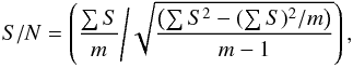 (3)where m is the number of pixels used in the wavelength interval. We then weighted each spectrum by the weight proportional to (S/N)2 and normalized to the mean S/N of all spectra that were used. The rebinning of the electronic spectra and preparation of input data for KOREL was carried out with the program HEC35D written by PH2.
Using the ephemeris (2) and the orbital parameters derived with SPEL, we run a number of tests. First, we kept all elements fixed and ran the program for several different values of the semi-amplitude K1 to find out which one gives the lowest sum of squares of the residuals. This indicated K1 ~ 81 km s-1 as the optimal value (see the upper panel of Fig. 1). Keeping this value fixed, we carried out a similar mapping to obtain the best guess for the mass ratio q = K1/K2. The result is shown in the bottom panel of Fig. 1 (q ~ 0.66).
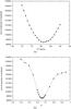 |
Fig. 1 Sum of squares of residuals for trial KOREL solutions with fixed elements as a function of a) the semi-amplitude K1 (upper panel), and b) the mass ratio K1/K2 (lower panel). |
Starting with these values, we then carried out a series of KOREL solutions, but now allowing the free convergence of the epoch Tmin.I, semi-amplitude K1, and the mass ratio q = K1/K2 and variously kicking away the initial values from the adopted values. The solution that gives the lowest sum of squares of residuals are shown in Table 3, and the corresponding disentangled spectra of the components are shown in Fig. 2. We note that the SPEL solution based on RVs measured in SPEFO does not differ significantly from the optimal KOREL solution.
The KOREL program does not provide error estimates of individual parameters. However, certain error estimates can be obtained as follows. First, since there is a good agreement between the results from RVs directly measured with SPEFO and those from KOREL, one can adopt the K and q errors from the SPEL solution in Table 2 as being quite representative of real uncertainties. Secondly, we can also estimate uncertainties of K1 and K2 from the RV measurements given in Table 1. According to the values in Table 1, our RV measurements have mean errors of 0.63 and 1.1 km s-1 for the primary and secondary components, respectively. These values are also in good agreement with the K errors in Table 2. Thirdly, a close inspection of the rather flat minima in Fig. 1 suggests errors of σK1 = 2 km s-1 and σq = 0.02 for K1 and q, respectively. Therefore, finally, we adopt the average errors of σK1 = 1.1 km s-1, σK2 = 1.3 km s-1, and σq = 0.015 for K1, K2 and q, respectively.
Best trial orbital solution with KOREL (see the text for the estimation procedure of the error bars).
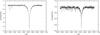 |
Fig. 2 Disentangled spectra of primary (left panel) and secondary (right panel) components obtained with KOREL . |
3.5. A comparison of disentangled and observed spectra with synthetic ones
To obtain the estimates of the effective temperatures, gravity accelerations, and projected rotational velocities from spectroscopy, we used two independent procedures.
First we used a program which compares synthetic spectra with disentangled or observed spectra of multiple systems to estimate radiative properties of its components (see Nasseri et al. 2014, for the details). The program uses several pre-calculated grids of synthetic spectra. The primary falls within parameters covered with grid POLLUX (Palacios et al. 2010) and the secondary falls within grid AMBRE (de Laverny et al. 2012). The wavelength band Δλ ∈ { 6330−6695 } Å was fitted. The optimized parameters were the effective temperature, the projected rotational velocity, the systemic radial velocity, and the relative luminosity3 of both components. The result is presented in Col. 2 of Table 4.
Uncertainties of fitted parameters were estimated with a Monte Carlo simulation, which was carried out as follows: 1) The continuum σc noise was estimated for each disentangled spectrum, using the same procedure as the previous section. 2) An artificial Gaussian noise with σ = σc was added to the disentangled profile. 3) The adjusted disentangled spectrum was fitted. This procedure was repeated 500 times and the errors were estimated from the distribution of results from all runs. These uncertainties do not reflect the need for the re-normalization of disentangled profiles. This step especially affects the width of Hα line and, consequently, the obtained parameters, particularly the gravitational acceleration and the projected velocity. The gravitational acceleration was estimated from the light curve solution and fixed during the fitting of disentangled spectra, but the projected rotational velocity was fitted.
Properties of the binary components of BD+36°3317 estimated from the comparison of the disentangled (Col. 2) and observed (Col. 3) spectra with synthetic ones (see the text for details).
To test the reliability of the estimated projected rotational velocity, another fit that followed the same procedure was computed, but the fitted wavelength range was only Δλ ∈ { 6342−6350;6368−6374 } Å. This region contains a pair of silicon lines Si ii 6347 Å and Si ii 6371 Å, which should be unaffected by the re-normalization uncertainty. The optimal rotational velocities are v1sini = 32.55 ± 0.59 km s-1, and v2sini = 22.1 ± 1.2 km s-1. This shows that the true uncertainty of the rotational velocity of secondary is ~10 km s-1.
As an independent approach to determine the effective temperatures of the components we used the program COMPO2 written by Frasca et al. (2006), which combines two reference spectra for both components for given effective temperatures, radial velocities (or systemic velocity), projected rotational velocities, and gravitational accelerations and compare the combined spectrum to the observed spectrum of a binary system. To achieve this, we used the reference spectra taken from Valdes et al. (2004) and tried to reproduce our observed spectrum taken at maximum orbital elongations (0.75 phase). COMPO2 tries to minimize the residuals between observed and composite spectra to find optimal parameter values for effective temperature and fractional flux contributions. The results of this procedure are listed in Col. 3 of Table 4. As seen from the table, both methods estimate almost the same values for the primary’s effective temperature. However the relative contributions of the components to the total luminosity in the spectral regions under consideration do differ somewhat from each other.
3.6. Simultaneous solution of light and radial velocity curves with PHOEBE
The final solution to obtain the binary masses, radii, and luminosities was carried out with the program PHOEBE . The RVs presented in Table 1 and all four LCs obtained from the literature (Johnson V observations were taken from Violat-Bordonau 2008, and the Johnson U, B, and V observations from Özdarcan et al. 2012, and priv. comm.) are solved simultaneously. For the temperatures of the components, the bolometric albedos A1,2 and gravitational darkening coefficients g1,2 were taken from Claret (2001, 1998), respectively. The limb-darkening coefficients x1,2 were computed automatically by PHOEBE from internal tables of the programme which were generated according to the models given by Castelli & Kurucz (2004). Convergence was allowed for the epoch of primary minimum Tmin.I, the orbital period P, the semi-major axis of the relative orbit a, systemic velocity Vγ, orbital inclination i, dimensionless surface potentials of the components Ω1 and Ω2, the effective temperature of the secondary component Teff,2, mass ratio q, and relative monochromatic luminosities of the primary component L1 in individual photometric pass-bands.
To refine the temperatures of the primary component, which we obtained in previous sections, we applied an Teff,1 search procedure. We subsequently solved the RV and LC curves simultaneously for a number of fixed values of Teff,1 between 10 000–11 250 K. The run of the weighted sum of the square of residuals (χ2 = [ ΣW(O–C)2 ]) thus obtained as a function of the effective temperature of the primary is shown in Fig 3. As can be seen from the figure, χ2 has its lowest value around Teff,1 = 10 450 K which agrees with Teff,1 = 10 750 ± 450 K given by Özdarcan et al. (2012) within the uncertainty bars, and so for the final solution we adopted Teff,1 = 10 450 K.
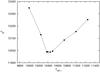 |
Fig. 3 Search for the best value of the effective temperature (Teff,1) for primary component with PHOEBE solutions. |
The final results are shown in Table 5. The values of the parameters P, i, a, and q given in Table 5 correspond to K1 = 82.23 ± 0.82 km s-1and K2 = 121.29 ± 0.85 km s-1, which match the results of SPEL and KOREL in previous subsections. The model light and RV curves are compared with the observations in Fig. 4. They show a small Rossiter (rotational) effect (Rossiter 1924) in the RV curves near the phases of binary eclipses.
Final solution for the physical properties of BD+36°3317.
3.7. Physical properties of the system
Using the results of the final solution from Table 5, we calculated the basic physical properties of the components. These are summarised in Table 6. The masses of the primary and secondary components are consistent with the spectral types A3 V and F2 V, respectively. Using the observed V-band magnitude outside the eclipses and (U − B) and (B − V) colours given by Özdarcan et al. (2012), the relative luminosities from the PHOEBE solution, and the bolometric corrections from Gray (2005), we calculated the de-reddened magnitudes, colours, distance moduli and the distances of the components. These are also given in Table 6. Considering that the primary is much brighter than the secondary, we weighted the individually derived distances to the components with their luminosities and estimated the mean distance to the system as  = 330 ± 29 pc.
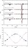 |
Fig. 4 a) Observed (dots) and theoretical (solid lines) light curves of BD+36°3317. The theoretical curves are calculated using the parameters given in Table 5. b) A phase plot of RVs of BD+36°3317. Black dots and open circles denote the RVs of the primary and secondary, respectively. Solid lines show the theoretical RV curves derived with the PHOEBE program (see Sect. 3.6). We note the presence of a small Rossiter (rotational) effect. |
In Fig. 5 we show the positions of the components in the Hertzsprung-Russell (HR) diagram, with the zero age main sequence (ZAMS) line taken from Claret & Giménez (1989) for the solar composition. Both components are clearly located very close to ZAMS. In the same figure, the evolutionary tracks by Bertelli et al. (2009) for the composition of z = 0.017, y = 0.3 are also shown. These agree well with the masses of the components that we derived.
Basic properties of BD+36°3317 .
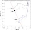 |
Fig. 5 Positions of the primary (black filled dot) and secondary (blue filled triangle) components in the HR diagram. The red solid line represents the ZAMS from the Claret & Giménez (1989) models. The evolutionary tracks labelled with the corresponding model masses are taken from Bertelli et al. (2009). |
4. Is BD+36°3317 a member of the δ Lyr cluster?
Although there were some doubts about the very existence of the δ Lyr (Stephenson 1) cluster, Kharchenko et al. (2005), Kharchenko et al. (2013) and Dias et al. (2014) have included δ Lyr cluster in their open clusters (OCs) catalogues. Kharchenko et al. (2004, 2013) use three different criteria for the membership of individual stars in each considered cluster: proper motions Pkin, photometric properties Pph, and spatial properties Psp of the stars, respectively. For δ Lyr cluster, Kharchenko et al. (2013) give E(B − V)= 0m.031, RV = −27.5 km s-1, and distance d = 373 pc.
For an independent determination of the reddening and distance modulus of the open cluster δ Lyr, we decided to use only the stars that have membership probabilities over 50% in each of the three criteria used by Kharchenko et al. (2004). They are listed in Table 7. To fit the theoretical main sequence of the cluster in both colour–colour (CC) and colour–magnitude (CM) diagrams, we consider only these highly probable cluster members. The theoretical main sequences in CC and CM diagrams are shifted along the axes to fit the observed main sequences.
We used the theoretical main sequence given by Johnson (1966) and Schmidt-Kaler (1982) and represented it by a sixth order polynomial. Then we fitted this polynomial to the most probable members of δ Lyr cluster. After this, we carried out a searching procedure for the colour excess E(B − V). To do so, we first shifted the theoretical main sequence along the (B − V) axis for a given value of E(B − V), and then determined the value of the distance modulus by hand, to find the smallest standard deviation σ(m − M) for the differences between the theoretical and observed main sequences. Consequently, the resulting value of the distance modulus corresponds to the smallest error of distance d for the value of the corresponding E(B − V), too. The procedure was then repeated with a new value for the reddening. We show the variation of the smallest standard deviation σ(m − M), which was obtained for the cluster’s distance modulus as a function of the reddening in Fig. 6. This shows that an error of 0.01 mag for E(B − V) is acceptable and we adopted E(B − V) = 0m.06 ± 0.01 for the cluster. This value of the reddening corresponds to an apparent distance modulus (m − M)v = 7m.98 ± 0.13. Adopting the visual extinction Av = 3.1E(B − V), we obtain Av = 0.19 mag and the distance of δ Lyr cluster of 362 ± 22 pc, lower than that found by Kharchenko et al. (2013). In addition, we estimate a reddening of about 0m.04 in (U − B) from CC diagram, as shown in Fig. 7. In Fig. 7 the photometric UBV data were taken from Eggen (1968) and Bronkalla (1963) and the stars in the vicinity of the δ Lyr cluster are shown, as well as the most probable cluster members and the primary and secondary components of BD+36°3317.
Most probable members of the δ Lyr cluster.
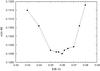 |
Fig. 6 Iterative determination of the optimal E(B − V); see text for details. |
Kharchenko et al. (2005) give the cluster radius as 0.87 degrees and RV = −21.6 km s-1 (compared with −27.5 km s-1 in Kharchenko et al. 2013). Only four stars have the RV measurements in the δ Lyr cluster field. These stars and the RV measurements are given in Table 8. Low membership probabilities are given for δ2 Lyr and HD 174959 in (Kharchenko et al. 2013). However the probabilities of the membership for δ1 Lyr and HD 175081 are higher. The systemic RV of BD+36°3317 from our solution agrees with δ1 Lyr, but not with HD 175081. Nevertheless, the locations of the components of BD+36°3317 in both CC and CM diagrams (see Fig. 7), are in good agreement with the other highly probable members of the cluster. Also, Kharchenko et al. (2004, 2013) classify the system as a highly probable member. The adopted distance, which is the luminosity-weighted average of the distances obtained for the components from Table 6, is 330 ± 29 pc, consistent with the cluster’s distance (362 ± 22 pc) within the quoted errors. So, we conclude that BD+36°3317 is one of the most probable members of the δ Lyr cluster, although obtaining more observations, in particular RVs, for more cluster member candidates is still very desirable.
At this point we decided to estimate the age of the cluster. So we tried to obtain best isochrone fitting for the cluster by using only the most probable members given in Table 7. To do so, we considered both the turn-off point and the slope of the main sequence together. We compared our CM diagram with the YZVAR Padova Isochrones produced by Bertelli et al. (2009). We obtained the best fit for the isochrone of (y,z) = (0.3,0.017) for the cluster. Finally, as seen in Fig. 8, the age of the cluster is between log t = 7.4 and 7.5. So we accepted an age of about 3 × 10⁷ yrs for the cluster. This value is also in good accordance with the evolutionary status of BD+36°3317, as pointed out in Sect. 3.7.
RV measurements of stars in δ Lyr cluster.
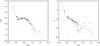 |
Fig. 7 CC (left panel) and CM (right panel) diagrams for δ Lyr cluster. The solid lines represent the theoretical ZAMS shifted in both axes by appropriate amounts (see the text).The triangle and square symbols denote the primary and secondary component, respectively. Black dots represent the stars in the field of the cluster while the big blue dots represent the stars having high membership probability. |
5. Conclusion
Obtaining and studying the first series of electronic spectra of BD+36°3317 and solving the RV curves of both binary components together with already published light curves, we obtained the first complete set of basic physical properties for this eclipsing binary, which is a probable member of δ Lyr cluster. The results can be summarised as follows.
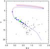 |
Fig. 8 HR diagram of δ Lyr cluster. The triangles and squares denote the primary and secondary components, respectively. Black dots represent the stars in the field of the cluster and the big blue dots, the stars having high membership probability. Padova isochrones taken from Bertelli et al. (2009) are shown for the reddening of 0m.06 and the apparent distance modulus of 7m.98. The isochrones shown are for 25 (red line) and 32 (blue line) Myrs and for the chemical composition (y,z) = (0.3,0.017). |
-
1.
The masses, radii, effective temperatures, and absolute luminosities summarised in Table 6 show that both components of BD+36°3317 are little evolved from the ZAMS and compatible with the published evolutionary models of Bertelli et al. (2009).
-
2.
The spin-orbit synchronisation for our solution would predict the projected rotational velocities of 20.7 and 17.2 km s-1 for the primary and secondary, respectively. This does not contradict the values we estimated from the line profiles, taking their associated errors into consideration.
-
3.
We reinforce the conclusion that BD+36°3317 is a probable member of the δ Lyr cluster. Both binary components seem to agree with the other members of δ Lyr cluster on the main sequence in CM diagram.
-
4.
Using the de-reddened magnitudes from our solution individually for both components, we derived the weighted mean distance of BD+36°3317 of 330 ± 29 pc. This distance is within the boundaries of the cluster distance estimated from CM diagram of δ Lyr cluster and, if the membership of BD+36°3317 in the cluster can be confirmed definitively, it would represent the most accurate estimate for the distance of the δ Lyr cluster.
The program has never been published but was carefully tested and used in several publications. http://astro.troja.mff.cuni.cz/ftp/hec/SPEL90/spel.pdf
The program and a manual to it can be downloaded from http://astro.troja.mff.cuni.cz/ftp/hec/HEC35
Acknowledgments
We thank to Dr. O. Özdarcan for sharing his photometric data of BD+36°3317 with us, and to Dr. Ö. Çakırlı for his support concerning the program COMPO2 for temperature searching process with the composite spectra method. The visit of EK in Praha and Ondřejov was supported by The Scientific and Technological Research Council of Turkey (TÜBİTAK) by the fellowship of BİDEP-2214 International Doctoral Research Fellowship Programme. She thanks colleagues in the Astronomical Institute of the Charles University and Astronomical Institute of the Academy of Sciences of the Czech Republic for their hospitality and help during her stay. Research of P.H., M.W., and J.N. was supported by grants P209/10/0715 and GA15-02112S of the Czech Science Foundation and the research of J.N. was additionally supported with grant No. 250015 of Grant Agency of the Charles University in Prague. We benefited from the use of the SIMBAD database and the VizieR service operated at CDS, Strasbourg, France and the NASA’s Astrophysics Data System Bibliographic Services and the WEBDA open cluster database.
References
- Anthony-Twarog, B. J. 1984, AJ, 89, 655 [NASA ADS] [CrossRef] [Google Scholar]
- Bertelli, G., Nasi, E., Girardi, L., & Marigo, P. 2009, A&A, 508, 355 [NASA ADS] [CrossRef] [EDP Sciences] [Google Scholar]
- Bronkalla, W. 1963, Astron. Nachr., 287, 249 [NASA ADS] [CrossRef] [Google Scholar]
- Castelli, F., & Kurucz, R. L. 2004, ArXiv e-prints [arXiv:astro-ph/0405087] [Google Scholar]
- Claret, A. 1998, A&AS, 131, 395 [NASA ADS] [CrossRef] [EDP Sciences] [Google Scholar]
- Claret, A. 2001, MNRAS, 327, 989 [NASA ADS] [CrossRef] [Google Scholar]
- Claret, A., & Giménez, A. 1989, A&AS, 81, 1 [NASA ADS] [Google Scholar]
- de Laverny, P., Recio-Blanco, A., Worley, C. C., & Plez, B. 2012, A&A, 544, A126 [NASA ADS] [CrossRef] [EDP Sciences] [Google Scholar]
- Dias, W. S., Monteiro, H., Caetano, T. C., et al. 2014, A&A, 564, A79 [NASA ADS] [CrossRef] [EDP Sciences] [Google Scholar]
- Eggen, O. J. 1968, ApJ, 152, 77 [NASA ADS] [CrossRef] [Google Scholar]
- Eggen, O. J. 1972, ApJ, 173, 63 [NASA ADS] [CrossRef] [Google Scholar]
- Eggen, O. J. 1983, MNRAS, 204, 391 [NASA ADS] [CrossRef] [Google Scholar]
- Frasca, A., Guillout, P., Marilli, E., et al. 2006, A&A, 454, 301 [NASA ADS] [CrossRef] [EDP Sciences] [Google Scholar]
- Gontcharov, G. A. 2006, Astron. Lett., 32, 759 [NASA ADS] [CrossRef] [Google Scholar]
- Gray, D. F. 2005, The Observation and Analysis of Stellar Photospheres, 3rd edn. (UK: Cambridge University Press), 533 [Google Scholar]
- Hadrava, P. 1995, A&AS, 114, 393 [NASA ADS] [Google Scholar]
- Hadrava, P. 1997, A&AS, 122, 581 [NASA ADS] [CrossRef] [EDP Sciences] [Google Scholar]
- Hadrava, P. 2004, Publications of the Astronomical Institute of the Czechoslovak Academy of Sciences, 92, 15 [Google Scholar]
- Hadrava, P. 2009, ArXiv e-prints [arXiv:#0909.0172] [Google Scholar]
- Harmanec, P., Koubský, P., Nemravová, J. A., et al. 2015, A&A, 573, A107 [NASA ADS] [CrossRef] [EDP Sciences] [Google Scholar]
- Horn, J., Kubát, J., Harmanec, P., et al. 1996, A&A, 309, 521 [NASA ADS] [Google Scholar]
- Johnson, H. L. 1966, ARA&A, 4, 193 [NASA ADS] [CrossRef] [Google Scholar]
- Kharchenko, N. V., Piskunov, A. E., Röser, S., Schilbach, E., & Scholz, R.-D. 2004, Astron. Nachr., 325, 740 [NASA ADS] [CrossRef] [Google Scholar]
- Kharchenko, N. V., Piskunov, A. E., Röser, S., Schilbach, E., & Scholz, R.-D. 2005, A&A, 438, 1163 [NASA ADS] [CrossRef] [EDP Sciences] [MathSciNet] [Google Scholar]
- Kharchenko, N. V., Scholz, R.-D., Piskunov, A. E., Röser, S., & Schilbach, E. 2007, Astron. Nachr., 328, 889 [NASA ADS] [CrossRef] [Google Scholar]
- Kharchenko, N. V., Piskunov, A. E., Schilbach, E., Röser, S., & Scholz, R.-D. 2013, A&A, 558, A53 [NASA ADS] [CrossRef] [EDP Sciences] [Google Scholar]
- Nasseri, A., Chini, R., Harmanec, P., et al. 2014, A&A, 568, A94 [NASA ADS] [CrossRef] [EDP Sciences] [Google Scholar]
- Özdarcan, O., Sipahi, E., & Dal, H. A. 2012, New A, 17, 483 [NASA ADS] [CrossRef] [Google Scholar]
- Palacios, A., Gebran, M., Josselin, E., et al. 2010, A&A, 516, A13 [NASA ADS] [CrossRef] [EDP Sciences] [Google Scholar]
- Prša, A., & Zwitter, T. 2005, ApJ, 628, 426 [NASA ADS] [CrossRef] [Google Scholar]
- Prša, A., & Zwitter, T. 2006, Ap&SS, 304, 347 [NASA ADS] [CrossRef] [Google Scholar]
- Rossiter, R. A. 1924, ApJ, 60, 15 [NASA ADS] [CrossRef] [Google Scholar]
- Schmidt-Kaler, T. 1982, Landolt-Börnstein: Numerical Data and Functional Relationships in Science and Technology – New Series “Gruppe/Group 6 Astronomy and Astrophysics” Vol. 2 Schaifers/Voigt: Astronomy and Astrophysics/Astronomie und Astrophysik “Stars and Star Clusters/Sterne und Sternhaufen [Google Scholar]
- Škoda, P. 1996, in Astronomical Data Analysis Software and Systems V, eds. G. H. Jacoby, & J. Barnes, ASP Conf. Ser., 101, 187 [Google Scholar]
- Škoda, P., & Hadrava, P. 2010, in Binaries – Key to Comprehension of the Universe, eds. A. Prša, & M. Zejda, ASP Conf. Ser., 435, 71 [Google Scholar]
- Stephenson, C. B. 1959, PASP, 71, 145 [NASA ADS] [CrossRef] [Google Scholar]
- Valdes, F., Gupta, R., Rose, J. A., Singh, H. P., & Bell, D. J. 2004, ApJS, 152, 251 [NASA ADS] [CrossRef] [Google Scholar]
- Violat-Bordonau, F. & Arranz-Heras, T. 2008, Information Bulletin onVariable Stars, 5900, 7 [Google Scholar]
- Wilson, R. E., & Devinney, E. J. 1971, ApJ, 166, 605 [NASA ADS] [CrossRef] [Google Scholar]
All Tables
Best trial orbital solution with KOREL (see the text for the estimation procedure of the error bars).
Properties of the binary components of BD+36°3317 estimated from the comparison of the disentangled (Col. 2) and observed (Col. 3) spectra with synthetic ones (see the text for details).
All Figures
|
Fig. 1 Sum of squares of residuals for trial KOREL solutions with fixed elements as a function of a) the semi-amplitude K1 (upper panel), and b) the mass ratio K1/K2 (lower panel). |
| In the text | |
|
Fig. 2 Disentangled spectra of primary (left panel) and secondary (right panel) components obtained with KOREL . |
| In the text | |
|
Fig. 3 Search for the best value of the effective temperature (Teff,1) for primary component with PHOEBE solutions. |
| In the text | |
|
Fig. 4 a) Observed (dots) and theoretical (solid lines) light curves of BD+36°3317. The theoretical curves are calculated using the parameters given in Table 5. b) A phase plot of RVs of BD+36°3317. Black dots and open circles denote the RVs of the primary and secondary, respectively. Solid lines show the theoretical RV curves derived with the PHOEBE program (see Sect. 3.6). We note the presence of a small Rossiter (rotational) effect. |
| In the text | |
|
Fig. 5 Positions of the primary (black filled dot) and secondary (blue filled triangle) components in the HR diagram. The red solid line represents the ZAMS from the Claret & Giménez (1989) models. The evolutionary tracks labelled with the corresponding model masses are taken from Bertelli et al. (2009). |
| In the text | |
|
Fig. 6 Iterative determination of the optimal E(B − V); see text for details. |
| In the text | |
|
Fig. 7 CC (left panel) and CM (right panel) diagrams for δ Lyr cluster. The solid lines represent the theoretical ZAMS shifted in both axes by appropriate amounts (see the text).The triangle and square symbols denote the primary and secondary component, respectively. Black dots represent the stars in the field of the cluster while the big blue dots represent the stars having high membership probability. |
| In the text | |
|
Fig. 8 HR diagram of δ Lyr cluster. The triangles and squares denote the primary and secondary components, respectively. Black dots represent the stars in the field of the cluster and the big blue dots, the stars having high membership probability. Padova isochrones taken from Bertelli et al. (2009) are shown for the reddening of 0m.06 and the apparent distance modulus of 7m.98. The isochrones shown are for 25 (red line) and 32 (blue line) Myrs and for the chemical composition (y,z) = (0.3,0.017). |
| In the text | |
Current usage metrics show cumulative count of Article Views (full-text article views including HTML views, PDF and ePub downloads, according to the available data) and Abstracts Views on Vision4Press platform.
Data correspond to usage on the plateform after 2015. The current usage metrics is available 48-96 hours after online publication and is updated daily on week days.
Initial download of the metrics may take a while.