| Issue |
A&A
Volume 587, March 2016
|
|
|---|---|---|
| Article Number | A40 | |
| Number of page(s) | 11 | |
| Section | Extragalactic astronomy | |
| DOI | https://doi.org/10.1051/0004-6361/201526760 | |
| Published online | 15 February 2016 | |
The rate and luminosity function of long gamma ray bursts
1
Universitá degli Studi dell’Insubria,
via Valleggio 11,
22100
Como,
Italy
e-mail:
alessio.pescalli@brera.inaf.it
2
INAF–Osservatorio Astronomico di Brera, via E. Bianchi
46, 23807
Merate,
Italy
3
INAF–IASF Milano, via E. Bassini 15, 20133
Milano,
Italy
4
GEPI, Observatoire de Paris, PSL Research University, CNRS,
Université Paris Diderot, Sorbonne
Paris Cité, Place Jules Janssen, 92195
Meudon,
France
5
Universitá degli Studi di Milano-Bicocca,
Piazza della Scienza 3,
20126
Milano,
Italy
6
AIM, UMR 7158 CEA/DSM-CNRS-Université Paris Diderot,
Irfu/Service d’Astrophysique,
Saclay, 91191
Gif-sur-Yvette Cedex,
France
Received: 16 June 2015
Accepted: 13 November 2015
We derive, adopting a direct method, the luminosity function and the formation rate of long Gamma Ray Bursts through a complete, flux-limited, sample of Swift bursts which has a high level of completeness in redshift z (~82%). We parametrise the redshift evolution of the GRB luminosity as L = L0(1 + z)k and we derive k = 2.5, consistently with recent estimates. The de-evolved luminosity function φ(L0) of GRBs can be represented by a broken power law with slopes a = −1.32 ± 0.21 and b = −1.84 ± 0.24 below and above, respectively, a break luminosity L0,b = 1051.45±0.15 erg/s. Under the hypothesis of luminosity evolution we find that the GRB formation rate increases with redshift up to z ~ 2, where it peaks, and then decreases in agreement with the shape of the cosmic star formation rate. We test the direct method through numerical simulations and we show that if it is applied to incomplete (both in redshift and/or flux) GRB samples it can misleadingly result in an excess of the GRB formation rate at low redshifts.
Key words: gamma-ray burst: general
© ESO, 2016
1. Introduction
Since the discovery of gamma ray bursts (GRBs), one of the most important questions has related to their distance scale (i.e. whether galactic or cosmological) which had immediate implications on their associated luminosities and energetics. By using the afterglow detection (Costa et al. 1997; van Paradijs et al. 1997) and first redshift measurements, GRBs were proven to be cosmological sources with large isotropic equivalent luminosities that exceed, in a few cases, 1054 erg s-1. The pinpointing of the GRB afterglow, made available by the fast slewing of the Swift satellite (Gehrels et al. 2004), combined with the intense efforts to acquire early time optical spectra from the ground, allowed us to measure the redshifts z of GRBs with an average efficiency of 30%. Among these, GRB 090423 (with a spectroscopic z = 8.2 – Salvaterra et al.2009a; Tanvir et al. 2009) and GRB 090429B (with photometric redshift z = 9.4 – Cucchiara et al. 2011) represent the furthest objects of stellar origin known to date.
Two key properties that characterise the population of GRBs are (a) their cosmic rate ψ(z) (GRB formation rate GRBFR, hereafter), representing the number of bursts per unit comoving volume and time as a function of redshift, and (b) their luminosity function φ(L) (LF) , which represents the relative fraction of bursts with a certain luminosity. Here, with φ(L) we refer to the luminosity probability density function (PDF) defined as dN(L)/dL/Ntot.
Recovering ψ(z) and φ(L) of GRBs allows us to test the nature of their progenitor (e.g. by a comparison with the cosmic star formation rate) and to study the possible presence of subclasses of GRBs at the low end of the luminosity function (e.g. Liang et al. 2007, see also Pescalli et al. 2015). These two functions were derived for the population of long GRBs (e.g. Daigne et al. 2006; Guetta & Della Valle 2007; Firmani et al. 2004; Salvaterra & Chincarini 2007; Salvaterra et al. 2009b, 2012; Wanderman & Piran 2010; Yu et al. 2015; Petrosian et al. 2015) through different methods and samples of bursts (Sect. 2). For the population of short GRBs, ψ(z) and φ(L) have been less securely constrained (e.g. Guetta & Piran 2005, 2006; Nakar et al. 2006; Berger 2014; D’Avanzo et al. 2014) because of the limited number of bursts with measured redshifts.
However, ψ(z) and φ(L) cannot be derived straightforwardly using all GRBs with known redshift since these samples are affected by observational bias. Specific methods that correct for any bias should be adopted. The main approaches that have been used so far (Sect. 2) agree on the shape of the luminosity function (typically represented by a broken power law) but lead to remarkably different results on the cosmic GRB rate (particularly at low redshifts). Independent of the method used to recover these two functions, most of the previous studies (see however Salvaterra et al. 2012) adopt either heterogeneous samples (i.e. including GRBs detected by diverse satellites/GRB detectors which have different sensitivities) and/or incomplete samples. In particular, incompleteness is induced by several effects, such as the variation of the trigger efficiency and the redshift measurement. Accounting for instrumental effects is extremely difficult in practice.
An alternative is to work with complete samples at the expense of the number of GRBs in the sample. Salvaterra et al. (2012; S12) define a complete flux-limited sample of GRBs (called BAT6) that was detected by Swift which, despite containing a relatively small number of GRBs, has a high redshift completeness and has been extensively used to test various prompt and afterglow properties of GRBs in an unbiased way (Campana et al. 2012; Covino et al. 2013; D’Avanzo et al. 2012; Ghirlanda et al. 2012; Melandri et al. 2012, 2014; Nava et al. 2012; Vergani et al. 2015).
The aim of this work is to derive φ(L) and ψ(z) through this complete sample of GRBs that was detected by Swift. We summarise the main different approvan paradijsaches that have been used in the literature to derive the luminosity function and the formation rate of GRBs (Sect. 2) and present the updated sample used in this work in Sect. 3. In Sect. 4, we adopt the C− direct method (Lynden-Bell 1971) to derive the φ(L) and ψ(z) and compare it with previous results . Throughout the paper we assume a standard ΛCDM cosmological model with Ωm = 0.3 and ΩΛ = 0.7 with H0 = 70 km s-1 Mpc-1. We use the symbol L to indicate the isotropic equivalent luminosity Liso , omitting for simplicity the subscript “iso”.
2. φ(L) and ψ(z) of long GRBs
The number of GRBs detectable by a given instrument above its sensitivity flux limit S can be expressed as  (1)where Ω and T are the instrument field of view and time of operation, respectively, and dV/dz is the differential comoving volume. Here, z(Lmax,S) is the maximum redshift at which a burst with Lmax can still be above the instrumental flux limit S; Llim(S,z) is the minimum observable luminosity as a function of z (i.e. that corresponds to a flux above S). A unique spectrum has been assumed, given the limit flux S, to obtain well-defined values for z(Lmax,S) and Llim(S,z).
If φ(L) and ψ(z) are known, it is possible to derive from Eq. (1) the flux distribution of the population of GRBs observable by a given detector, knowing its instrumental parameters. By reversing this argument, one can assume the functional forms of φ(L) and ψ(z) (e.g. specified through a set of free parameters) and constrain them by fitting the model flux distribution, i.e. N( >S) to the observed flux distribution of a given instrument. This indirect method has been used to infer the luminosity function (e.g. Firmani et al. 2004; Salvaterra & Chincarini 2007; Salvaterra et al. 2009b, 2012) by fitting, e.g. the flux distribution of the large population of GRBs detected by BATSE.
The number of free parameters, if both φ(L) and ψ(z) are to be constrained, can be large. One possibility is to assume that, based on the massive star progenitor origin of long bursts, the GRB cosmic rate traces the cosmic star formation rate, i.e. ψ(z)∝ψ⋆(z). In this way, the method allows us to derive the free parameters of φ(L) by fitting the result of Eq. (1) to large, statistically significant, samples of observed GRBs. The assumed ψ(z) can be tested by fitting the observed redshift distribution of a sample of bursts with measured z.
In the simplest scenario, the two functions φ(L) and ψ(z) are independent. However, more realistic analyses also considered the possible evolution of either the luminosity function or the GRB formation rate with redshift. For example, in the case of luminosity evolution, the luminosity of the burst depends on z through the relation L(z) = L0(1 + z)k (luminosity evolution scenario). The luminosity function at a particular redshift z can be constructed by assuming luminosity evolution as at z = 0, i.e. φ(L,z) = φ(L0(1 + z)k). Alternatively, the GRB formation rate ψ(z) varies with redshift with a similar analytical dependence ψ(z) ∝ ψ⋆(z)(1 + z)d (density evolution scenario). This means that the progenitor characteristics evolve with z and that the ratio of the GRB-formation rate to the cosmic star-formation rate is not constant. Among the drawbacks of this method is that it relies on the assumption of a specific functional form of φ(L) (commonly, simple functions, e.g. power law, broken power law or power law with a cutoff at low luminosities, have been adopted) and it allows for only evolution of the luminosity or of the rate to be tested independently.
Salvaterra et al. (2012) applied the indirect method to a complete sample of GRBs that were detected by Swift (Sect. 3). They find that either a luminosity evolution with k = 2.1 ± 0.6 or a density evolution with d = 1.7 ± 0.5 can reproduce the flux distribution of BATSE bursts and the redshift distribution of the Swift complete sample. However, they cannot discriminate between these two scenarios. They derive the luminosity function φ(L) by testing two analytical models: a power-law with an exponential cut-off at low luminosities and a broken power law (BPL), φ(L) ∝ (L/Lb)a,b, where a and b are the slopes of the power law below and above the break Lb), adopting a minimum GRB luminosity Lmin = 1049 erg/s. For the BPL model they found  ,
,  ,
,  erg/s in the case of the luminosity evolution scenario (parameters refer to LF at z = 0) and
  ,
,  ,
,  erg/s in the case of the density evolution scenario.
The alternative method is based on the direct derivation of the φ(L) and ψ(z) from observed samples of GRBs with measured z and L. This method has been inherited from the studies of the luminosity function of quasars and blazars (e.g. Chiang & Mukherjee 1998; Maloney & Petrosian 1999; Singal et al. 2012, 2013) and it has been applied to GRBs (Lloyd & Petrosian 1999; Kocevski & Liang 2006). Wanderman & Piran (2010) adopt a maximum likelihood estimator to derive the discrete luminosity function and cosmic formation rate. They use the sample of ~100 GRBs detected by Swift with measured redshift (through optical afterglow absorption lines and photometry). Despite this sample possibly suffering from incompleteness, they derive φ(L) (extending from 1050 erg/s up to 1054 erg/s), which can be represented by a broken power law with a = −1.2, b = −2.4 and Lb = 1052.5 erg/s. Similarly, they also derive the discrete GRB formation rate ψ(z) which can be represented by a broken power law as a function of (1 + z) with indices  and
and  peaking at
  . This rate is consistent with the SFR of Bouwens et al. (2009) for z ≲ 3. They assume that the luminosity is independent of redshift.
More recently, Yu et al. (2015 – Y15 hereafter) and Petrosian et al. (2015 – P15 hereafter) apply a statistical method to reconstruct the discrete φ(L) and ψ(z) from a sample of Swift bursts with measured redshifts. They both find a strong luminosity evolution with k ~ 2.3. Their results converge towards a cumulative luminosity function described by a broken power law with α = −0.14 ± 0.02, β = −0.7 ± 0.03, Lb = 1.43 × 1051 erg/s (Y15) and α = −0.5, β = −2.2, Lb = 1051 erg/s (P15). These indices (α and β) are the slopes of the cumulative luminosity function which is linked to the differential one through the integral  . Therefore, for a BPL luminosity function, the slopes of the differential form are (a,b) = (α−1,β−1).
Intriguingly, they find that the GRB rate is flat or decreases from the local Universe up to z = 1, which is at odds with previous works. When compared to the SFR, this behaviour would imply a relative excess of the GRB formation rate with respect to ψ∗(z) at z ≤1 (if both are normalised to their respective peaks). They dub this behaviour the excess of GRBs at low redshifts. This result is also puzzling because it is completely at odds with the findings of the works based on the properties of GRB host galaxies. In fact, Vergani et al. (2015), Perley et al. (2015, 2016a,b), Krühler et al. (2015) and Schulze et al. (2015), performed multi-wavelength and spectroscopic studies on the properties (stellar masses, luminosities, SFR, and metallicity) of GRB host galaxies of different complete GRB samples and compared them to those of the star-forming galaxies selected by galaxy surveys. All their results clearly indicate that at z< 1 only a small fraction of the star formation produces GRBs.
Both P15 and Y15 apply a statistical method (Efron & Petrosian 1992) to remove the redshift dependence of the luminosity that has been induced by the flux-cut in the selected GRB sample. They use GRBs detected by Swift with measured redshifts. However, while Yu et al. (2015) work with the bolometric luminosity of GRBs, Petrosian et al. (2015) adopt the luminosity in the Swift/BAT (15–150 keV) energy band. Y15 use all GRBs detected by Swift with a measured redshift and well constrained spectral parameters; despite their relatively large number of objects (~130), this is an incomplete sample. P15 account for incompleteness by cutting their sample to a relatively large flux level, at the expense of the total number of bursts, i.e. working with ~200 out of 250 events with measured z.
Independent of the method adopted to recover φ(L) and ψ(z), one key point is the definition of the sample. S12 show the importance of working with complete samples of GRBs (see also Hjorth et al. 2012). Here we start with the so-called BAT6 Swift sample (S12) and extend it with additional bursts that satisfy its selection criteria (Sect. 3). We will then use it to derive the luminosity function and the cosmic GRB formation rate (Sect. 4).
3. BAT6 extended version
The BAT6 complete sample as defined in S12 was composed of 58 Swift GRBs with (i) favourable observing conditions for their redshift measurement as proposed in Jakobsson et al. (2006) and (ii) a peak photon flux P ≥ 2.6 ph cm-2 s-1 (integrated over the 15–150 keV Swift/BAT energy band). This sample, which is complete in flux by definition, after selection turned out to be also highly complete (~90%) in redshift (i.e. 52 out of 58 bursts have z).
The study of the isotropic equivalent luminosity L of the bursts of the BAT6 sample requires knowledge of their broadband prompt emission spectrum. Nava et al. (2012) collected the 46 out of 52 GRBs, within the BAT6, with measured Ep and z. Six bursts with measured z did not have Ep measurements. One of the main drawbacks of the narrow/soft energy range of the BAT instrument is the difficulty in measuring the peak Ep of the νFν spectrum for the several bursts it detects. Other instruments (e.g. Konus/Wind – Aptekar et al.1995, Fermi/GBM – Meegan et al. 2009 or Suzaku/WAM – Yamaoka et al. 2009) compensate for this deficiency, by means of their wide energy range, and measuring a spectrum that extends from few keV to several MeV.
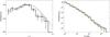 |
Fig. 1 Left panel: GRB formation rate ψ(z) obtained with the C− method using the BAT6ext sample (black solid line). The dashed red line and the dot-dashed cyan line are the SFR models of Hopkins & Beacom (2006) and Cole et al. (2001) shown here for reference. All the curves are normalised to their maxima. Right panel: luminosity function φ(L0) obtained with the C− method using the BAT6ext sample (black solid line). The best fit model describing this function is a broken power-law (dashed green line) with (a = −1.32 ± 0.21, b = −1.84 ± 0.24, Lb = 1051.45 ± 0.15 erg/s). The orange dot-dashed line is the luminosity function obtained by S12 in the case of pure luminosity evolution. |
Sakamoto et al. (2009) showed that for Swift bursts with measured Ep there is a correlation between the slope of the spectrum αPL (when fitted with a single power-law model) and the peak energy Ep (measured by fitting a curved model). With the aim of enlarging the sample of Nava et al. (2012), we estimate Ep of six bursts of the BAT6, whose BAT spectrum is fitted by a single power law, through this relation (Sakamoto et al. 2009). We also verified that the values obtained are consistent with those of the other bursts. (We performed the K−S test finding a probability of ~70% that the two sets of peak energies originate from the same distribution.) We found that all but one GRB, i.e. 070306, have  =
=  (1 + z), which is consistent with the upper/lower limit reported in Nava et al. (2012). Therefore, we were the first to extend the BAT6 sample of Nava et al. (2012) with measured z and L to 50 out of 58 bursts.
Since the construction of the BAT6, other bursts that satisfy its selection criteria were detected by Swift. Moreover, some bursts that were already present in the original BAT6 sample were re–analysed and either their redshifts and/or their spectral properties were revised. Therefore, our first aim was to revise the BAT6 sample. In particular, the revision of eight redshifts is here included (marked in italics in the table – with their luminosity updated). The revised BAT6 sample then contains 56 out of 58 GRBs with measured z and 54 out of 58 that also a bolometric isotropic luminosity L. Taking only the redshift into consideration, the sample is ~97% complete while, if we also require the knowledge of L, the completeness level is only slightly smaller (~93%).
Then, we extended the BAT6 revised sample with new events that have been detected since 2012, and which satisfy the observability criteria of Jakobsson et al. (2006). The extended sample contains 99 GRBs. We collected the spectral parameters of the new GRBs in the existing literature. For events (6 out of 41 bursts) with only a Swift single power law spectrum, we estimated Ep through the Sakamoto et al. (2009) relation. The BAT6 extended (BAT6ext) counts 82 out of 99 GRBs with z (and 81 out of 99 with z and L. Its completeness in redshift is ~82%.
The BAT6ext is presented in Table B.1. The first 58 bursts are the original BAT6, while the others constitute the extension. For each GRB, Table B.1 shows the redshift z, the spectral parameters (high and low photon indices α and β, and the rest frame peak energy ), the peak flux with the relative energy band, and the isotropic equivalent luminosity L. The spectrum is a cut-off power-law (CPL) if only the low energy photon index α is reported and a band function, if the high energy photon index β is also given. When z is not measured, we report the observed peak energy. The luminosities reported in the table are only calculated in the [1−104] keV rest frame energy range for those GRBs having both z and Ep.
4. Luminosity function and GRB formation rate
In this section we will apply the C− method as originally proposed by Lynden-Bell (1971) and applied to GRBs by e.g. Yonetoku et al. (2004, 2014), Kocevski & Liang (2006), and Wu et al. (2012). This method is based on the assumption that the luminosity is independent of the redshift. However, as discussed in Petrosian et al. (2015), a strong luminosity evolution could be present in the GRB population. Efron & Petrosian (1992) proposed a non-parametric test to estimate the degree of correlation of the luminosity with redshift induced by the flux in a flux-limited sample. This is also the case of the BAT6ext sample and the first step is to quantify the degree of correlation. Indeed Yu et al. (2015) and Petrosian et al. (2015) find that the luminosity evolves with redshift within their samples as  (Y15) or (1 + z)2.3 ± 0.8 (P15). We applied the same method of Y15 and P15 (also used in Yonetoku et al. 2004, 2014) to the BAT6ext sample: we define the luminosity evolution L = L0(1 + z)k (as in Y15), where L0 is the de-evolved luminosity, and compute the modified Kendall correlation coefficient (as defined in Efron & Petrosian 1992). Consistent with the results of Y15 and P15, we find k = 2.5. Similar results were obtained through the indirect method (see Sect. 2) by S12 using the BAT6 sample.
We can now define the de-evolved luminosities L0 = L/ (1 + z)k for every GRBs and apply the Lynden–Bell C− method to derive the cumulative luminosity function Φ(L0) and the GRB formation rate ψ(z).
For the ith GRB in the BAT6ext sample, described by its (L0,i,zi), we consider the subsample Ji = { j | L0,j>L0,i ∩ zj<zmax,i } and call Ni the number of GRBs it contains. Similarly, we define the subsample  and we call Mi the number of GRBs it contains. Hence, Llim,i is the minimum luminosity corresponding to the flux limit S of the sample at the redshift zi; zmax,i is the maximum redshift at which the ith GRBs with luminosity L0,i can be observed, i.e. with flux above the limit S.
In this case, since the BAT6 sample was selected according to the limiting flux computed in the observer frame Swift/BAT [15−150] keV energy band, Llim and zmax are computed by adopting for each GRB its own spectrum and applying the corresponding K-correction. This approach introduces a small scatter in the cut in the L−z plane (which means a non-unique equivalent bolometric limit flux) and this has a very small impact in the computation of Llim and zmax and, consequently, in the definition of subsamples J and J′.
Through Mi and Ni we can estimate the cumulative luminosity function Φ(L0) and the cumulative GRB redshift distribution ζ(z):  (2)and
  (3)From the latter we can derive the GRB formation rate as
 ![\begin{equation} \psi(z)=\frac{{\rm d}\zeta(z)}{{\rm z}}(1+z)\left[\frac{{\rm d}V(z)}{{\rm d}z}\right]^{-1} \label{rate} , \end{equation}](/articles/aa/full_html/2016/03/aa26760-15/aa26760-15-eq116.png) (4)where dV(z)/dz is the differential comoving volume. The differential luminosity function φ(L0) is obtained by deriving the cumulative one Φ(L0).
(4)where dV(z)/dz is the differential comoving volume. The differential luminosity function φ(L0) is obtained by deriving the cumulative one Φ(L0).
Note that Mj and Nj are equal to 0 for bursts that are at the edge of the distribution in the L−z plane. In these cases, we discard the contribution of these bursts to the products of Eqs. (2) and (3).
The functions φ(L0) and ψ(z) are shown in Fig. 1. Errors on φ(L0) are computed by propagating the errors on the cumulative one and assuming Poisson statistics. The errors on the ψ(z) are computed from the number n of GRBs within the redshift bin. We assume that the relative error  is the same as that affecting ψ(z).
5. Results
The luminosity function φ(L0) obtained with the BAT6ext sample is shown in Fig. 1 (right panel) by the black symbols. Data are normalised to the maximum. The best-fit model (green dashed line in Fig. 1 – right panel) is represented by a broken power-law function with a = −1.32 ± 0.21, b = −1.84 ± 0.24, Lb = 1051.45 ± 0.15 erg/s (where a and b represent the slopes of the power-law above and below Lb – χ2/ d.o.f. = 0.47). By way of comparison, in Fig. 1 we also show the luminosity function derived in S12 through the indirect method (described in Sect. 2) assuming pure luminosity evolution (, , erg/s). This model is consistent with the result obtained in our analysis.
The GRB formation rate ψ(z) that was obtained with the BAT6ext is shown by the black symbols in Fig. 1 (left panel). The green dashed and the cyan dotted-dashed lines are, respectively, the SFR of Hopkins & Beacom (2006) and Cole et al. (2001). Data and models are normalised to their peak. Contrary to the results reported in P15 and Y15, the ψ(z) that we derive increases up to z ~ 2. This trend is consistent with the independent estimates obtained through host galaxy studies.
Results of the analysis for the Ep−L correlation.
The BAT6ext sample has a smaller completeness in redshift (~82%) with respect to the revised BAT6 (~97%). We checked if this could in some way modify the shape of ψ(z). For this reason we also computed the ψ(z) using only the 56 objects of the revised BAT6 sample, which turns out to be slightly steeper both at low and high redshifts than the one obtained with the BAT6ext, but it is totally consistent within the errors. We conclude that the lower completeness in redshift of the BAT6ext does not introduce any strong bias in the obtained ψ(z) and φ(L0).
5.1. The Ep – L correlation
In this work we extended and updated the BAT6 complete sample, taking it to 99 objects. We then calculated the isotropic equivalent luminosities for all bursts with z measured and well constrained spectral parameters (81 out of 99 objects have both L and z). On this basis, we show in Fig. 2 the correlation Ep−L (Yonetoku et al. 2004; Nava et al. 2012) based on the updated sample. We also compared the total sample of all bursts with L and z measured (187 objects – updated to GRB 140907A). The correlation was fitted using the bisector method (Isobe et al. 1990) in the barycentre of points for both the total and the BAT6ext sample, respectively. We also estimate the scatter of the distribution of the points around the correlation (computed perpendicular to the correlation itself), the Spearman’s rank correlation coefficient and the associated chance probability. These results are reported in Table 1.
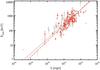 |
Fig. 2 Ep−L correlation. Grey points and the red empty squares represent the total and BAT6ext complete sample. The solid gray line and the dot-dashed line are the best-fit (obtained with the bisector method applied in the barycentre of points) results for the total and BAT6ext complete sample respectively. |
6. Monte Carlo test of the C− method
We now test the C− method used to derive ψ(z) and φ(L0). Through a Monte Carlo simulation (similar to e.g. Ghirlanda et al. 2015) we explore how well the method adopted in Sect. 4 can recover the input assumptions, i.e. ψ(z) and LF φ(L). In particular, we show that if the sample used is highly incomplete, the resulting GRBFR and LF can differ significantly from those that were input. In particular, incomplete samples (either in flux and/or redshift) may produce a misleading excess of low redshift GRBs with respect to the assumed ψ(z).
We simulate GRBs that are distributed in redshift according to the GRB formation rate ψ(z) of Li (2008) (see also Hopkins & Beacom 2006):  (5)where ψ(z), in units of M⊙yr-1Mpc-3, represents the formation rate of GRBs and we assume it can extend to z ≤ 10. We stress that for the scope of the present test any other functional form of ψ(z) could be assumed.
We adopt a luminosity function φ(L), as obtained by Salvaterra et al. (2012), from a complete sample of Swift GRBs: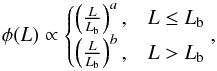 (6)composed of two power laws with a break at Lb. We adopt arbitrary parameter values: a = −1.2, b = −1.92 and Lb = 5×1050 erg s-1. We further assume an evolution in the luminosity proportional to (1 + z)k with k = 2.2. Here, L is the bolometric luminosity of the simulated bursts, and therefore
  is the corresponding bolometric flux. For this reason we do not need to assume any spectral shape for the simulated GRBs to obtain the values of Llim and zmax. Also for φ(L) we use this functional form but any other function could be assumed for the scope of the present test.
With these two assumptions, we simulate a sample of GRBs with a flux limit Flim = 5 × 10⁻⁸ erg cm-2 s-1 and we analyse it with the C− method. Accounting for the truncation of the sample, we recover the luminosity evolution in the form (1 + z)k, with k ~ 2.2, using the statistical method of Efron & Petrosian (1992).
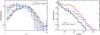 |
Fig. 3 Left panel: GRB-formation rate (normalised to its peak) for the simulated population of GRBs with flux limit 5 × 10⁻⁸ erg cm-2 s-1 (black symbols). The GRB-formation rate assumed in the simulation is shown by the dashed green line. The red symbols show the results obtained from the same sample using, for the analysis, a flux limit factor of 5 smaller than the real one. Blue symbols are obtained by mimicking the sample incompleteness by removing some GRBs randomly near the flux threshold adopted for the sample selection. Right panel: cumulative luminosity function, normalised to the first bin. The black, red, and blue symbols are the same as for the left panel. The assumed luminosity function is shown by the dashed green line. |
Then we work with the de-evolved GRB luminosities L0 = L/ (1 + z)2.2 and derive the GRB formation rate ψ(z) and the luminosity function φ(L0) through the C− method proposed by Lynden-Bell (1971). The left-hand panel of Fig. 3 shows that we recover the GRB formation rate in Eq. (5) that we adopted in the simulation. Similarly, the right-hand panel of Fig. 3 shows that we also recover the luminosity function that we adopted in the simulated sample (Eq. (6) – shown by the dashed green line in Fig. 3).
We then tested what happens if we apply the same method to an incomplete sample. Firstly we applied the C− method to the same simulated sample, which is built to be complete to Flim = 5 × 10⁻⁸ erg cm-2 s-1, from which we randomly removed a fraction of the bursts close to Flim. This new sample is clearly incomplete to Flim. The results are shown in Fig. 3. We find that the GRB formation rate ψ(z) is flat at low redshifts (i.e. below z = 2), which shows a clear excess with respect to the assumed function (see Fig. 3). The luminosity function is flatter than the assumed one (see Fig. 3 right-hand panel).
Similar results were obtained by assuming for the derivation of ψ(z) and φ(L0) a flux limit which is a factor of five smaller than that used to construct the simulated sample, which is another way to make the sample artificially incomplete. The results are shown in the panels of Fig. 3. We note that in this second test, the sample used is the same but it is analysed through the C− method, assuming it is complete with respect to a flux limit which is smaller (a factor of five) than the one corresponding to its real completeness (i.e. 5 × 10⁻⁸ erg cm-2 s-1).
These simulations show that if the samples adopted are highly incomplete in flux, an excess at the low redshift end of the GRB formation rate and a flatter luminosity function are obtained.
7. Summary and discussion
We set out to derive the luminosity function of long GRBs and their formation rate. To this aim we apply a direct method (Lynden-Bell 1971) and its specific version already applied to GRBs, e.g. Yonetoku et al. (2004, 2014), Kocevski & Liang (2006), Wu et al. (2012), P15, Y15. This is the first time this method has been applied to a well-defined sample of GRBs that is complete in flux and 82% complete in redshift.
We built our sample of long GRBs starting from the BAT6 complete sample (Salvaterra et al. 2012): this was composed of 58 GRBs detected by the Swift satellite satisfying the multiple observational selection criteria of Jakobsson et al. (2006) and having a peak photon flux P ≥ 2.6 ph cm-2 s-1. Here, we updated the redshift measurement of eight GRBs of the BAT6 (marked in italics in Table B.1) and accordingly revise their luminosities. Then, we updated this sample to GRB 140703A ending with 99 objects. We collected their redshift measurements and spectral parameters from the literature (see Table B.1). The BAT6ext sample has a redshift completeness of ~82% (82 out of 99 burst with z measured) and counts 81 out of 99 bursts with well determined L. Using the BAT6ext sample, we also tested the Ep−L Yonetoku correlation and compared it to the total sample of all bursts of measured L and Ep (Fig. 2). The slopes of the correlations are 0.5 and 0.54 for the total and BAT6ext sample, respectively, which is consistent with each other within 1σ errors (see Table 1). Also the scatter of the points distribution around the correlations are similar (0.29 and 0.28 for the total and BAT6ext sample, respectively).
We analyzed the BAT6ext sample, searching for a possible luminosity evolution that was induced by the flux threshold using the method proposed by Efron & Petrosian (1992). We found that the L−z correlation, which was introduced by the truncation because of the flux limit, can be described as L = L0(1 + z)k with k = 2.5. This result is in agreement with what has been found by other authors (Yonetoku et al. 2004; Wu et al. 2012; P15; Y15). Taking the BAT6ext sample, after de-evolving the luminosities for their redshift dependence, we find that:
-
the luminosity function φ(L0) is a monotonic decreasing function that is well described by a broken power-law with slopes a = −1.32 ± 0.21 and b = −1.84 ± 0.24 below and above, respectively, and a characteristic break luminosity Lb = 1051.45 ± 0.15 erg/s (see right-hand panel of Fig. 1). This result (shape, slopes, and characteristic break) is consistent with the luminosity function found by S12 (see Fig. 1, right-hand panel).
-
The cosmological GRB formation rate ψ(z) (see left-hand panel of Fig. 1) increases from low redshifts to higher values, peaking at z ~ 2 and decreases at higher redshifts. This trend is consistent with the shape of the SFR of Hopkins & Beacom (2006) and Cole et al. (2001) (see Fig. 1). Our results on ψ(z) are in contrast with the GRBFR recently found by P15 and Y15, who report the existence of an excess of low redshift GRBs when applying the same method to differently selected GRB samples.
The luminosity evolution we found is huge (but in agreement with the findings of Yonetoku et al. 2004; Wu et al. 2012; P15; Y15) and, therefore, it might be difficult to justify theoretically (Daigne et al. 2006). In fact, this could imply an evolution with redshift of either the physical processes leading to the emission of γ-rays and/or an evolution in the physical properties of the progenitor (even if the GRB-formation rate seems to follow the SFR, as obtained in this work).
However, the result that GRBs evolve in luminosity should not be interpreted as the proof that GRBs had experienced a pure luminosity evolution. It is beyond the scope of this work to demonstrate which type of evolution the GRBs experienced. In fact, the C− method assumes the independence between L and z and the non-parametric method of Efron & Petrosian (1992), which was used to get the de-evolved luminosities, assigns the whole evolution to the luminosity. For this reason, we are not able to distinguish between a luminosity or density evolution (see also Salvaterra et al. 2012) and probably the true solution resides in a combination of the two. The possible density evolution case requires the investigation of the applicability of similar methods to the GRB samples and will be the subject of a forthcoming work (Pescalli et al., in preparation).
Finally, intrigued by the different results with respect to Y15 and P15, we performed Monte Carlo simulations to test the robustness of the C− method. We showed that this method can correctly recover the LF φ(L0) and the GRBFR ψ(z) assumed in the simulation, but only if the sample of GRBs it is applied to is complete in flux and has a high level of completeness in redshift. Using incomplete samples or a sample that is incomplete in redshift, the resulting GRBFR and LF can turn out different from the assumed ones. Indeed, this could account for the excess of the rate of GRBs at low redshift, as recently reported.
Acknowledgments
We thank the referee for comments that help us to improve the manuscript. We acknowledge the 2011 PRIN-INAF grant for financial support. We acknowledge the financial support of the UnivEarthS Labex program at Sorbonne Paris Cité (ANR-10-LABX-0023 and ANR-11-IDEX-0005-02). G.G. thanks the Observatoire de Paris (Meudon) for support and hospitality during the completion of this work. We thank S. Campana and G. Tagliaferri for contributing to useful discussions.
References
- Aptekar, R. L., Frederiks, D. D., Golenetskii, S. V., et al. 1995, Space Sci. Rev., 71, 265 [NASA ADS] [CrossRef] [Google Scholar]
- Avni, Y., & Bahcall, J. N. 1980, ApJ, 235, 694 [NASA ADS] [CrossRef] [Google Scholar]
- Barthelmy, S. D., Baumgartner, W. H., Cummings, J. R., et al. 2012a, GRB Coordinates Network, 13990 [Google Scholar]
- Barthelmy, S. D., Sakamoto, T., Markwardt, C. B., et al. 2012b, GRB Coordinates Network, 13120 [Google Scholar]
- Barthelmy, S. D., Baumgartner, W. H., Cummings, J. R., et al. 2013, GRB Coordinates Network, 14469 [Google Scholar]
- Baumgartner, W. H., Barthelmy, S. D., Cummings, J. R., et al. 2011, GRB Coordinates Network, 12424 [Google Scholar]
- Baumgartner, W. H., Barthelmy, S. D., Cummings, J. R., et al. 2014, GRB Coordinates Network, 16473 [Google Scholar]
- Berger, E. 2014, ARA&A, 52, 43 [NASA ADS] [CrossRef] [Google Scholar]
- Bouwens, R. J., Illingworth, G. D., Franx, M., et al. 2009, ApJ, 705, 936 [NASA ADS] [CrossRef] [Google Scholar]
- Campana, S., Salvaterra, R., Melandri, A., et al. 2012, MNRAS, 421, 1697 [NASA ADS] [CrossRef] [Google Scholar]
- Castro-Tirado, A. J., Sanchez-Ramirez, R., Gorosabel, J., et al. 2013, GRB Coordinates Network, 14796 [Google Scholar]
- Castro-Tirado, A. J., Cunniffe, R., Sanchez-Ramirez, R., et al. 2014, GRB Coordinates Network, 16505 [Google Scholar]
- Chiang, J., & Mukherjee, R. 1998, ApJ, 496, 752 [NASA ADS] [CrossRef] [Google Scholar]
- Cole, S., Norberg, P., Baugh, C. M., et al. 2001, MNRAS, 326, 255 [NASA ADS] [CrossRef] [Google Scholar]
- Connaughton, V. 2011, GRB Coordinates Network, 12133 [Google Scholar]
- Costa, E., Frontera, F., Heise, J., et al. 1997, Nature, 387, 783 [NASA ADS] [CrossRef] [Google Scholar]
- Covino, S., Melandri, A., Salvaterra, R., et al. 2013, MNRAS, 432, 1231 [NASA ADS] [CrossRef] [Google Scholar]
- Cucchiara, A., & Levan, A. J. 2011, GRB Coordinates Network, 12761 [Google Scholar]
- Cucchiara, A., & Perley, D. 2013, GRB Coordinates Network, 15144 [Google Scholar]
- Cucchiara, A., & Prochaska, J. X. 2012, GRB Coordinates Network, 12865 [Google Scholar]
- Cucchiara, A., Levan, A. J., Fox, D. B., et al. 2011, ApJ, 736, 7 [NASA ADS] [CrossRef] [Google Scholar]
- Cummings, J. R., Barthelmy, S. D., Baumgartner, W. H., et al. 2011, GRB Coordinates Network, 12749 [Google Scholar]
- Daigne, F., Rossi, E. M., & Mochkovitch, R. 2006, MNRAS, 372, 1034 [NASA ADS] [CrossRef] [Google Scholar]
- D’Avanzo, P., Salvaterra, R., Sbarufatti, B., et al. 2012, MNRAS, 425, 506 [NASA ADS] [CrossRef] [Google Scholar]
- D’Avanzo, P., Salvaterra, R., Bernardini, M. G., et al. 2014, MNRAS, 442, 2342 [NASA ADS] [CrossRef] [Google Scholar]
- de Ugarte Postigo, A., Gorosabel, J., Xu, D., et al. 2014, GRB Coordinates Network, 16310 [Google Scholar]
- de Ugarte Postigo, A., Tanvir, N., Sanchez-Ramirez, R., et al. 2013a, GRB Coordinates Network, 14437 [Google Scholar]
- de Ugarte Postigo, A., Xu, D., Malesani, D., et al. 2013b, GRB Coordinates Network, 15187 [Google Scholar]
- Efron, B., & Petrosian, V. 1992, ApJ, 399, 345 [NASA ADS] [CrossRef] [Google Scholar]
- Firmani, C., Avila-Reese, V., Ghisellini, G., & Tutukov, A. V. 2004, ApJ, 611, 1033 [NASA ADS] [CrossRef] [Google Scholar]
- Flores, H., Covino, S., de Ugarte Postigo, A., et al. 2013a, GRB Coordinates Network, 14493 [Google Scholar]
- Flores, H., Covino, S., Xu, D., et al. 2013b, GRB Coordinates Network, 14491 [Google Scholar]
- Frederiks, D. 2011, GRB Coordinates Network, 12137 [Google Scholar]
- Fynbo, J. P. U., Tanvir, N. R., Jakobsson, P., et al. 2014, GRB Coordinates Network, 16217 [Google Scholar]
- Gehrels, N., Chincarini, G., Giommi, P., et al. 2004, ApJ, 611, 1005 [NASA ADS] [CrossRef] [Google Scholar]
- Ghirlanda, G., Ghisellini, G., Nava, L., et al. 2012, MNRAS, 422, 2553 [NASA ADS] [CrossRef] [Google Scholar]
- Ghirlanda, G., Salvaterra, R., Ghisellini, G., et al. 2015, MNRAS, 448, 2514 [NASA ADS] [CrossRef] [Google Scholar]
- Golenetskii, S., Aptekar, R., Frederiks, D., et al. 2012, GRB Coordinates Network, 13412 [Google Scholar]
- Golenetskii, S., Aptekar, R., Frederiks, D., et al. 2013a, GRB Coordinates Network, 14487 [Google Scholar]
- Golenetskii, S., Aptekar, R., Frederiks, D., et al. 2013b, GRB Coordinates Network, 14575 [Google Scholar]
- Golenetskii, S., Aptekar, R., Frederiks, D., et al. 2013c, GRB Coordinates Network, 14720 [Google Scholar]
- Golenetskii, S., Aptekar, R., Frederiks, D., et al. 2013d, GRB Coordinates Network, 15145 [Google Scholar]
- Golenetskii, S., Aptekar, R., Frederiks, D., et al. 2013e, GRB Coordinates Network, 15203 [Google Scholar]
- Golenetskii, S., Aptekar, R., Frederiks, D., et al. 2013f, GRB Coordinates Network, 15413 [Google Scholar]
- Golenetskii, S., Aptekar, R., Frederiks, D., et al. 2013g, GRB Coordinates Network, 15452 [Google Scholar]
- Golenetskii, S., Aptekar, R., Mazets, E., et al. 2013h, GRB Coordinates Network, 14808 [Google Scholar]
- Golenetskii, S., Aptekar, R., Frederiks, D., et al. 2014a, GRB Coordinates Network, 15853 [Google Scholar]
- Golenetskii, S., Aptekar, R., Frederiks, D., et al. 2014b, GRB Coordinates Network, 16134 [Google Scholar]
- Golenetskii, S., Aptekar, R., Frederiks, D., et al. 2014c, GRB Coordinates Network, 16495 [Google Scholar]
- Gruber, D. 2012, GRB Coordinates Network, 12874 [Google Scholar]
- Guetta, D., & Della Valle, M. 2007, ApJ, 657, L73 [NASA ADS] [CrossRef] [Google Scholar]
- Guetta, D., & Piran, T. 2005, A&A, 435, 421 [Google Scholar]
- Guetta, D., & Piran, T. 2006, A&A, 453, 823 [NASA ADS] [CrossRef] [EDP Sciences] [Google Scholar]
- Hjorth, J., Malesani, D., Jakobsson, P., et al. 2012, ApJ, 756, 187 [NASA ADS] [CrossRef] [Google Scholar]
- Hopkins, A. M., & Beacom, J. F. 2006, ApJ, 651, 142 [NASA ADS] [CrossRef] [MathSciNet] [Google Scholar]
- Isobe, T., Feigelson, E. D., Akritas, M. G., & Babu, G. J. 1990, ApJ, 364, 104 [NASA ADS] [CrossRef] [EDP Sciences] [Google Scholar]
- Jakobsson, P., Levan, A., Fynbo, J. P. U., et al. 2006, A&A, 447, 897 [NASA ADS] [CrossRef] [EDP Sciences] [Google Scholar]
- Jenke, P. 2014a, GRB Coordinates Network, 16220 [Google Scholar]
- Jenke, P. 2014b, GRB Coordinates Network, 16512 [Google Scholar]
- Kocevski, D., & Liang, E. 2006, ApJ, 642, 371 [NASA ADS] [CrossRef] [Google Scholar]
- Krimm, H. A., Barlow, B. N., Barthelmy, S. D., et al. 2012, GRB Coordinates Network, 13634 [Google Scholar]
- Krühler, T., Malesani, D., Fynbo, J. P. U., et al. 2015, A&A, 581, A125 [NASA ADS] [CrossRef] [EDP Sciences] [Google Scholar]
- Li, L.-X. 2008, MNRAS, 388, 1487 [NASA ADS] [CrossRef] [Google Scholar]
- Liang, E., Zhang, B., Virgili, F., & Dai, Z. G. 2007, ApJ, 662, 1111 [NASA ADS] [CrossRef] [Google Scholar]
- Lien, A. Y., Barthelmy, S. D., Baumgartner, W. H., et al. 2013, GRB Coordinates Network, 14419 [Google Scholar]
- Lloyd, N. M., & Petrosian, V. 1999, ApJ, 511, 550 [NASA ADS] [CrossRef] [Google Scholar]
- Lynden-Bell, D. 1971, MNRAS, 155, 95 [NASA ADS] [CrossRef] [Google Scholar]
- Malesani, D., Xu, D., Fynbo, J. P. U., et al. 2014, GRB Coordinates Network, 15800 [Google Scholar]
- Maloney, A., & Petrosian, V. 1999, ApJ, 518, 32 [NASA ADS] [CrossRef] [Google Scholar]
- McGlynn, S. 2012, GRB Coordinates Network, 13997 [Google Scholar]
- Meegan, C., Lichti, G., Bhat, P. N., et al. 2009, ApJ, 702, 791 [NASA ADS] [CrossRef] [Google Scholar]
- Melandri, A., Sbarufatti, B., D’Avanzo, P., et al. 2012, MNRAS, 421, 1265 [NASA ADS] [CrossRef] [Google Scholar]
- Melandri, A., Covino, S., Rogantini, D., et al. 2014, A&A, 565, A72 [NASA ADS] [CrossRef] [EDP Sciences] [Google Scholar]
- Moskvitin, A., Burenin, R., Uklein, R., et al. 2014, GRB Coordinates Network, 16489 [Google Scholar]
- Nakar, E., Gal-Yam, A., & Fox, D. B. 2006, ApJ, 650, 281 [NASA ADS] [CrossRef] [Google Scholar]
- Nava, L., Salvaterra, R., Ghirlanda, G., et al. 2012, MNRAS, 421, 1256 [NASA ADS] [CrossRef] [MathSciNet] [Google Scholar]
- Palmer, D. M., Barthelmy, S. D., Baumgartner, W. H., et al. 2012a, GRB Coordinates Network, 12839 [Google Scholar]
- Palmer, D. M., Barthelmy, S. D., Baumgartner, W. H., et al. 2012b, GRB Coordinates Network, 13536 [Google Scholar]
- Palmer, D. M., Barthelmy, S. D., Baumgartner, W. H., et al. 2014, GRB Coordinates Network, 16423 [Google Scholar]
- Pelassa, V. 2013, GRB Coordinates Network, 14869 [Google Scholar]
- Perley, D. A., Perley, R. A., Hjorth, J., et al. 2015, ApJ, 801, 102 [NASA ADS] [CrossRef] [Google Scholar]
- Perley, D. A., Krühler, T., Schulze, S., et al. 2016a, ApJ, 817, 7 [NASA ADS] [CrossRef] [Google Scholar]
- Perley, D. A., Tanvir, N. R., Hjorth, J., et al. 2016b, ApJ, 817, 8 [NASA ADS] [CrossRef] [Google Scholar]
- Pescalli, A., Ghirlanda, G., Salafia, O. S., et al. 2015, MNRAS, 447, 1911 [NASA ADS] [CrossRef] [Google Scholar]
- Petrosian, V., Kitanidis, E., & Kocevski, D. 2015, ApJ, 806, 44 [NASA ADS] [CrossRef] [Google Scholar]
- Sakamoto, T., Sato, G., Barbier, L., et al. 2009, ApJ, 693, 922 [NASA ADS] [CrossRef] [Google Scholar]
- Sakamoto, T., Barthelmy, S. D., Baumgartner, W. H., et al. 2013, GRB Coordinates Network, 14959 [Google Scholar]
- Sakamoto, T., Barthelmy, S. D., Baumgartner, W. H., et al. 2014, GRB Coordinates Network, 15805 [Google Scholar]
- Salvaterra, R., & Chincarini, G. 2007, ApJ, 656, L49 [NASA ADS] [CrossRef] [Google Scholar]
- Salvaterra, R., Della Valle, M., Campana, S., et al. 2009a, Nature, 461, 1258 [NASA ADS] [CrossRef] [PubMed] [Google Scholar]
- Salvaterra, R., Guidorzi, C., Campana, S., Chincarini, G., & Tagliaferri, G. 2009b, MNRAS, 396, 299 [NASA ADS] [CrossRef] [Google Scholar]
- Salvaterra, R., Campana, S., Vergani, S. D., et al. 2012, ApJ, 749, 68 [NASA ADS] [CrossRef] [Google Scholar]
- Sanchez-Ramirez, R., Gorosabel, J., de Ugarte Postigo, A., & Gonzalez Perez, J. M. 2012, GRB Coordinates Network, 13723 [Google Scholar]
- Schmidl, S., Nicuesa Guelbenzu, A., Klose, S., & Greiner, J. 2012, GRB Coordinates Network, 13992 [Google Scholar]
- Schmidt, M. 1968, ApJ, 151, 393 [NASA ADS] [CrossRef] [Google Scholar]
- Schulze, S., Chapman, R., Hjorth, J., et al. 2015, ApJ, 808, 73 [NASA ADS] [CrossRef] [Google Scholar]
- Singal, J., Petrosian, V., & Ajello, M. 2012, ApJ, 753, 45 [NASA ADS] [CrossRef] [Google Scholar]
- Singal, J., Petrosian, V., Stawarz, Ł., & Lawrence, A. 2013, ApJ, 764, 43 [NASA ADS] [CrossRef] [Google Scholar]
- Stamatikos, M., Barthelmy, S. D., Baumgartner, W. H., et al. 2012, GRB Coordinates Network, 13559 [Google Scholar]
- Stanbro, M. 2014, GRB Coordinates Network, 16262 [Google Scholar]
- Tanvir, N. R., & Ball, J. 2012, GRB Coordinates Network, 13532 [Google Scholar]
- Tanvir, N. R., Fox, D., Fynbo, J., & Trujllo, C. 2012, GRB Coordinates Network, 13562 [Google Scholar]
- Tanvir, N. R., Fox, D. B., Levan, A. J., et al. 2009, Nature, 461, 1254 [NASA ADS] [CrossRef] [PubMed] [Google Scholar]
- Tanvir, N. R., Levan, A. J., Matulonis, T., & Smith, A. B. 2013, GRB Coordinates Network, 14567 [Google Scholar]
- Tanvir, N. R., Levan, A. J., Cucchiarra, A., Perley, D., & Cenko, S. B. 2014, GRB Coordinates Network, 16125 [Google Scholar]
- Tello, J. C., Sanchez-Ramirez, R., Gorosabel, J., et al. 2012, GRB Coordinates Network, 13118 [Google Scholar]
- Thoene, C. C., de Ugarte Postigo, A., Gorosabel, J., et al. 2012, GRB Coordinates Network, 13628 [Google Scholar]
- Ukwatta, T. N., Barthelmy, S. D., Baumgartner, W. H., et al. 2011, GRB Coordinates Network, 12352 [Google Scholar]
- Ukwatta, T. N., Barthelmy, S. D., Baumgartner, W. H., et al. 2012, GRB Coordinates Network, 14052 [Google Scholar]
- van Paradijs, J., Groot, P. J., Galama, T., et al. 1997, Nature, 386, 686 [NASA ADS] [CrossRef] [Google Scholar]
- Vergani, S. D., Salvaterra, R., Japelj, J., et al. 2015, A&A, 581, A102 [NASA ADS] [CrossRef] [EDP Sciences] [Google Scholar]
- Wanderman, D., & Piran, T. 2010, MNRAS, 406, 1944 [NASA ADS] [Google Scholar]
- Wiersema, K., Flores, H., D’Elia, V., et al. 2011, GRB Coordinates Network, 12431 [Google Scholar]
- Wolter, A., Caccianiga, A., della Ceca, R., & Maccacaro, T. 1994, ApJ, 433, 29 [NASA ADS] [CrossRef] [Google Scholar]
- Wu, S.-W., Xu, D., Zhang, F.-W., & Wei, D.-M. 2012, MNRAS, 423, 2627 [NASA ADS] [CrossRef] [Google Scholar]
- Xiong, S. 2012, GRB Coordinates Network, 12801 [Google Scholar]
- Xu, D., de Ugarte Postigo, A., Malesani, D., et al. 2013a, GRB Coordinates Network, 14956 [Google Scholar]
- Xu, D., Fynbo, J. P. U., Jakobsson, P., et al. 2013b, GRB Coordinates Network, 15407 [Google Scholar]
- Xu, D., Malesani, D., Tanvir, N., Kruehler, T., & Fynbo, J. 2013c, GRB Coordinates Network, 15450 [Google Scholar]
- Yamaoka, K., Endo, A., Enoto, T., et al. 2009, PASJ, 61, S35 [NASA ADS] [Google Scholar]
- Yonetoku, D., Murakami, T., Nakamura, T., et al. 2004, ApJ, 609, 935 [NASA ADS] [CrossRef] [Google Scholar]
- Yonetoku, D., Nakamura, T., Sawano, T., Takahashi, K., & Toyanago, A. 2014, ApJ, 789, 65 [NASA ADS] [CrossRef] [Google Scholar]
- Younes, G. 2013, GRB Coordinates Network, 14545 [Google Scholar]
- Younes, G., & Barthelmy, S. D. 2012, GRB Coordinates Network, 13721 [Google Scholar]
- Yu, H., Wang, F. Y., Dai, Z. G., & Cheng, K. S. 2015, ApJS, 218, 13 [NASA ADS] [CrossRef] [Google Scholar]
- Yu, H.-F. 2013, GRB Coordinates Network, 15064 [Google Scholar]
- Zauderer, A., & Berger, E. 2011, GRB Coordinates Network, 12190 [Google Scholar]
- Zhang, B.-B., & Bhat, N. 2014, GRB Coordinates Network, 15669 [Google Scholar]
Appendix A: The redshift integrated luminosity function
In this section we show how we derive the luminosity function of GRBs integrated over all the redshift space using the BAT6ext sample. This is not the typical luminosity function that is derived through indirect methods, since it is free from any functional form and only uses the 1 /Vmax concept, i.e. the maximum comoving volume within which a real burst with an observed luminosity can be detected by a given instrument. This is a generalisation of the ⟨ V/Vmax ⟩ method proposed by Schmidt (1968) and applied to quasars (see Avni & Bahcall 1980, for an exhaustive description).
However, the luminosity function obtained with this method is not the canonical φ(L), but it is the result of the integration of the latter convolved with the GRB formation rate ψ(z) over z. We call this function the convolved luminosity function Σ(L) (CLF). In thoery, the luminosity function may evolve with redshift (φ(L,z)). For this reason the shape of the CLF may be different from the shape of the canonical φ(L). It could simply be proportional to φ(L) only if the luminosity function does not evolve, either in luminosity or in density. Indeed, it is possible to express Σ(L) in terms of luminosity function and GRB formation rate 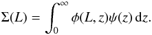 (A.1)The advantage is that this equation can be obtained directly from the data and it is extremely robust if derived through a flux-limited sample. Any evolution with redshift of the luminosity or density is in this CFL. We use the 80 out of 99 GRBs with both z and determined L, as reported in Table 1.
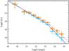 |
Fig. A.1 Blue-filled points represent the observed CLF Σ(L) while the orange squares represent the true CLF |
For each GRB of the BAT6ext sample with an associated L, we estimate the maximum volume Vmax within which the burst could still be detected because its flux would be larger than the chosen threshold, i.e. Plim = 2.6 ph cm-2 s-1 in the 15–150 keV energy band. The observed photon flux in the Swift/BAT energy band as a function of the varying redshift is  (A.2)where N(E) is the observed photon spectrum of each GRB and dL(z) is the luminosity distance at redshift z. The extremes of the integral in the denominator correspond to the same values adopted to compute L. The maximum redshift zmax corresponds to the redshift that satisfies P(zmax) = Plim.
Considering the typical Swift/BAT field of view Ω = 1.33 steradians and the time of activity of SwiftT ~ 9 yr that covers the BAT6ext sample, we can compute the rate ρi = 4π/ ΩTVmax,i for each GRB. We divided the observed range of luminosities in bins of equal logarithmic width Δ and estimate Σj(Lj) for each bin as  (A.3)where the sum is made over the bursts with luminosities Lj−Δ/2 ≤ Li ≤ Lj + Δ/2. The discrete convolved luminosity function is shown in Fig. A.1. The normalisation is obtained by also considering that the bursts in the BAT6ext sample represent approximately 1/3 of the total number of Swift detected GRBs with peak flux P ≥ 2.6 ph cm-2 s-1. We verified that the BAT6ext sample (99 objects) is representative in terms of peak-flux distribution of the larger population. The error bar associated with the discrete CLF are mainly related to the Poissonian error on the count within the luminosity bin (see also e.g. Wolter et al. 1994).
When computing individual rates, we used the mission-elapsed time T. However, this is the observer time frame and the rate should be corrected for the cosmological time dilation. This means that, at higher z, the same subset of sources should occur with a larger frequency. Therefore, we average out the elapsed time on the redshift interval [0,zmax] (A.4)and use it in the computation of Eq. (A.3). As shown in Fig. A.1, the true CLF
  is flatter than the observed one because, in general, the true elapsed time is less than the observed one. Moreover, the correction is more pronounced for high luminosity GRBs that are observable up to high redshifts.
The CLF obtained with the extended BAT6ext sample is shown in Fig. A.1. The observed CFL can be adequately represented by a broken power law function with slopes −1.39 ± 0.14 and −2.38 ± 0.41 below and above the break luminosity Lb = 1053.3 ± 0.3 erg/s (χ2/ d.o.f. = 1.04). When we correct for the cosmological time dilation, the true CLF appears slightly flatter (slopes −1.22 ± 0.1 and −2.09 ± 0.95 below and above the break Lb = 1053.3 ± 1 erg/s – χ2/ d.o.f. = 0.99).
We can look at this function as a redshift-integrated luminosity distribution. This is the most direct information that we can obtain from data, in fact, and it is obtained without any type of assumption or observational constraints. As with the flux distribution log N−log S and with the redshift distribution, it can be used as a constraint. The LF and the GRBFR obtained with other methods should reproduce this CLF once convolved together and integrated over z.
Appendix B: Additional table
BAT6ext GRB complete sample.
All Tables
All Figures
|
Fig. 1 Left panel: GRB formation rate ψ(z) obtained with the C− method using the BAT6ext sample (black solid line). The dashed red line and the dot-dashed cyan line are the SFR models of Hopkins & Beacom (2006) and Cole et al. (2001) shown here for reference. All the curves are normalised to their maxima. Right panel: luminosity function φ(L0) obtained with the C− method using the BAT6ext sample (black solid line). The best fit model describing this function is a broken power-law (dashed green line) with (a = −1.32 ± 0.21, b = −1.84 ± 0.24, Lb = 1051.45 ± 0.15 erg/s). The orange dot-dashed line is the luminosity function obtained by S12 in the case of pure luminosity evolution. |
| In the text | |
|
Fig. 2 Ep−L correlation. Grey points and the red empty squares represent the total and BAT6ext complete sample. The solid gray line and the dot-dashed line are the best-fit (obtained with the bisector method applied in the barycentre of points) results for the total and BAT6ext complete sample respectively. |
| In the text | |
|
Fig. 3 Left panel: GRB-formation rate (normalised to its peak) for the simulated population of GRBs with flux limit 5 × 10⁻⁸ erg cm-2 s-1 (black symbols). The GRB-formation rate assumed in the simulation is shown by the dashed green line. The red symbols show the results obtained from the same sample using, for the analysis, a flux limit factor of 5 smaller than the real one. Blue symbols are obtained by mimicking the sample incompleteness by removing some GRBs randomly near the flux threshold adopted for the sample selection. Right panel: cumulative luminosity function, normalised to the first bin. The black, red, and blue symbols are the same as for the left panel. The assumed luminosity function is shown by the dashed green line. |
| In the text | |
|
Fig. A.1 Blue-filled points represent the observed CLF Σ(L) while the orange squares represent the true CLF |
| In the text | |
Current usage metrics show cumulative count of Article Views (full-text article views including HTML views, PDF and ePub downloads, according to the available data) and Abstracts Views on Vision4Press platform.
Data correspond to usage on the plateform after 2015. The current usage metrics is available 48-96 hours after online publication and is updated daily on week days.
Initial download of the metrics may take a while.