| Issue |
A&A
Volume 586, February 2016
|
|
|---|---|---|
| Article Number | A148 | |
| Number of page(s) | 16 | |
| Section | Galactic structure, stellar clusters and populations | |
| DOI | https://doi.org/10.1051/0004-6361/201526484 | |
| Published online | 10 February 2016 | |
Controversial age spreads from the main sequence turn-off and red clump in intermediate-age clusters in the LMC⋆
1 Excellence Cluster Origin and Structure of the Universe, Boltzmannstr. 2, 85748 Garching bei München, Germany
e-mail: This email address is being protected from spambots. You need JavaScript enabled to view it.
2 Universitäts-Sternwarte München, Scheinerstraße 1, 81679 München, Germany
3 Astrophysics Research Institute, Liverpool John Moores University, 146 Brownlow Hill, Liverpool L3 5RF, UK
4 Space Telescope Science Institute, 3700 San Martin Drive, Baltimore, MD 21218, USA
5 European Southern Observatory, Karl-Schwarzschild-Straße 2, 85748 Garching bei München, Germany
6 Astronomical Institute Anton Pannekoek, Amsterdam University, Science Park 904, 1098 XH, Amsterdam, The Netherlands
7 Purple Mountain Observatory, Chinese Academy of Sciences, 210008 Nanjing, PR China
8 Kavli Institute for Astronomy and Astrophysics, Peking University, 100871 Beijing, PR China
9 Department of Astronomy, Peking University, 100871 Beijing, PR China
Received: 7 May 2015
Accepted: 26 October 2015
Abstract
Most star clusters at an intermediate age (1−2 Gyr) in the Large and Small Magellanic Clouds show a puzzling feature in their color−magnitude diagrams (CMD) that is not in agreement with a simple stellar population. The main sequence turn-off of these clusters is much broader than expected from photometric uncertainties. One interpretation of this feature is that age spreads of the order of 200−500 Myr exist within individual clusters, although this interpretation is highly debated. Such large age spreads should affect other parts of the CMD, which are sensitive to age, as well. In this study, we analyze the CMDs of a sample of 12 intermediate-age clusters in the Large Magellanic Cloud that all show an extended turn-off using archival optical data taken with the Hubble Space Telescope. We fit the star formation history of the turn-off region and the red clump region independently. We find that in most cases, the age spreads inferred from the red clumps are smaller than those that result from the turn-off region. However, the age ranges that result from the red clump region are broader than expected for a single age. Only two out of 12 clusters in our sample show a red clump which seems to be consistent with a single age. As our results are ambiguous, by fitting the star formation histories to the red clump regions, we cannot ultimately tell if the extended main sequence turn-off feature is the result of an age spread or not. However, we do find that the width of the extended main sequence turn-off feature is correlated with the age of the clusters in a way which would be unexplained in the so-called age spread interpretation, but which may be expected if stellar rotation is the cause of the spread at the turn-off.
Key words: galaxies: star clusters: general / Magellanic Clouds / Hertzsprung-Russell and C-M diagrams / stars: evolution
Based on observations made with the NASA/ESA Hubble Space Telescope, and obtained from the Hubble Legacy Archive, which is a collaboration between the Space Telescope Science Institute (STScI/NASA), the Space Telescope European Coordinating Facility (ST-ECF/ESA), and the Canadian Astronomy Data Centre (CADC/NRC/CSA).
© ESO, 2016
1. Introduction
The traditional view of stellar clusters is that all stars in a cluster are born at the same time and have the same metallicity. This makes them ideal for stellar evolutionary models as all stars lie on a single isochrone in the color−magnitude diagram (CMD). However, high precision photometric and spectroscopic data of many clusters reveal features that are not in agreement with a simple stellar population (SSP). In the CMDs of globular clusters (GCs), broadened or double main sequences (MS) have been found that are caused by chemical anomalies (e.g., Gratton et al. 2012; Piotto et al. 2012; Milone et al. 2012a, 2013a). Different scenarios have been put forward to explain these abundance spreads inside GCs. The models propose either self-enrichment of the cluster caused by multiple bursts of star formation (e.g., D’Ercole et al. 2008; Decressin et al. 2009; de Mink et al. 2009; Conroy & Spergel 2011) or enrichment of low mass pre-MS stars by the ejecta of massive stars of the same generation (Bastian et al. 2013a). However, all models proposed so far have severe shortcomings (e.g., Larsen et al. 2012; Cabrera-Ziri et al. 2015; Bastian et al. 2015).
Additionally, a common feature in intermediate-age (1−2 Gyr) clusters in the Large and Small Magellanic Clouds (LMC and SMC) is a main sequence turn-off (MSTO) that is more extended than expected for an SSP (e.g., Mackey & Broby Nielsen 2007; Mackey et al. 2008; Milone et al. 2009; Goudfrooij et al. 2009, 2011a,b; Girardi et al. 2013; Piatti 2013). Many studies have interpreted this extended MSTO feature as an age spread of the order of 200−500 Myr inside the clusters (e.g., Goudfrooij et al. 2009, 2011a,b; Rubele et al. 2013; Correnti et al. 2014). However, the interpretation of star formation lasting for several hundred Myr is highly debated. A natural consequence of a prolonged star-formation history (SFH) would be a chemical enrichment of heavier elements in the younger generation of stars. To date, no significant abundance spread among stars in clusters that show an extended MSTO has been found (e.g., Mucciarelli et al. 2008, 2011, 2014; Mackey et al., in prep.).
To address the question of age spreads in intermediate-age massive LMC and SMC clusters, some studies have attempted to search for large age spreads or signs of ongoing star formation in young (<1 Gyr) massive clusters. Bastian et al. (2013b) analyzed a sample of 130 galactic and extragalactic young (10 Myr−1 Gyr) and massive (104−108M⊙) clusters and did not find evidence for active star formation (see also Peacock et al. 2013). Bastian & Silva-Villa (2013) fitted the resolved stellar population of NGC 1856 and NGC 1866, two young (180 Myr and 280 Myr) clusters in the LMC and concluded that they are compatible with an SSP. Niederhofer et al. (2015a) continued this study by analyzing the CMDs of eight more young massive LMC clusters with ages of between 20 Myr and 1 Gyr. They found no evidence for a significant age spread in any cluster from their sample. All clusters studied by Bastian & Silva-Villa (2013) and Niederhofer et al. (2015a) have properties similar to the extended MSTO intermediate-age clusters (cf. Fig. 6 in Niederhofer et al. 2015a). Cabrera-Ziri et al. (2014) analyzed the integrated spectrum of NGC 34 cluster 1, a ~100 Myr, 107 M⊙ cluster, and did not find evidence for multiple star-forming bursts or an extended SFH.
Goudfrooij et al. (2011b, 2014) put forward a model to explain how a prolonged period of star formation could have happened in intermediate-age LMC clusters. The authors propose a formation of a cluster that has several steps: In the first step a cluster, which is much more massive than observed today, forms within a single burst of star formation. This cluster is massive enough that it can retain the ejecta from evolved stars and is also able to accrete pristine gas from its surroundings, which is mixed with the processed gas from the ejecta. In the next step, a second generation of stars is formed within the cluster out of the mixed gas. This second burst of star formation lasts for 300 to 600 Myr. In the meantime the cluster looses almost all of its first generation stars (which make up to ~90% of the mass of the cluster). What is observed today is a cluster that is almost only composed of the second generation of stars that have age differences of approximately 300 to 600 Myr and that contains only ~10% of its initial mass.
To form subsequent generations of stars, clusters would need to reaccrete material from their surroundings. However, it is currently unclear how a cluster would actually do this, as young massive clusters are observed as being gas free from an early (<1−3 Myr) age and remain so (Hollyhead et al. 2015; Bastian & Strader 2014). Additionally, Cabrera-Ziri et al. (2015) searched for gas in three massive (>106 M⊙) clusters in the Antennae merging galaxies, with ages between 50−200 Myr, and did not detect any, which calls into doubt whether young massive clusters can host the necessary gas/dust reservoirs to form further generations of stars.
To explain the extended MSTOs, alternative scenarios have been suggested. Bastian & de Mink (2009) propose stellar rotation as being the cause of this phenomenon. This interpretation is later called into question by Girardi et al. (2011), based on calculations of isochrones for moderately rotating stars. They found that the longer lifetimes of rotating stars may cancel out the effect of changes in stellar structure that are caused by rotation. However, Yang et al. (2013) find that, in fact, rotation is able to explain the extended MSTO, depending on the efficiency of rotational mixing. For their analysis they use the Yale Rotating Evolution Code (YREC, Pinsonneault et al. 1989; Yang & Bi 2007).
If age spreads are the cause of the extended MSTO feature, it should affect other parts of the CMD that are sensitive to age, as well. Li et al. (2014) analyze the sub-giant branch (SGB) of NGC 1651, a ~2 Gyr old cluster in the LMC that shows an extended MSTO. They show that the SGB stars mostly follow the youngest isochrone that covers the spread in the MSTO (1.74 Gyr) with a spread in the SGB of 80 Myr at most. This spread is much smaller than would be inferred from the MSTO region (~450 Myr). Li et al. (2014) therefore conclude that the extended MSTO is not due to a prolonged star formation. Bastian & Niederhofer (2015) extend the study of Li et al. (2014) to NGC 1806 and NGC 1846, two ~1.4 Gyr old LMC clusters, which also show an extended MSTO. They use similar techniques to Li et al. (2014), but also take into account the morphology of the red clump. Their results show that the SGB and red clump morphology for both clusters is consistent with an SSP that follows the youngest isochrone through the MSTO region, agreeing with what was found by Li et al. (2014) for NGC 1651.
In this study we analyze the MSTO and red clump regions of a sample of 12 intermediate-age LMC clusters in a self-consistent way. We fit the SFH of the MSTO and the red clump region independently using the SFH code StarFISH (Harris & Zaritsky 2001).
The paper is organized as follows: in Sect. 2 we describe our data sample, the observations, reduction, and further processing of the data. In Sect. 3 we introduce our models and methods that we use for our analysis. In Sect. 4 we present the results. In Sect. 5 we analyze the extended MSTO widths as a function of the age of the cluster. Final conclusions are drawn in Sect. 6.
2. Observations and data processing
2.1. The data sample
The 12 LMC clusters in our total sample were observed with the HST Wide Field Channel at the Advanced Camera for Surveys (ASC/WFC) or the ultraviolet and visible (UVIS) channel of the Wide Field Camera 3 (WFC3) within the programs GO-9891 (PI: G. Gilmore), GO-10595 (PI : P.Goudfrooij), and GO-12257 (PI: L. Girardi), respectively. Both, the ACS/WFC and WFC3/UVIS are composed of two CCD chips with 4096 × 2048 pixels and 4096 × 2051 pixels in size, with a gap of about 50 pixels in between. The pixel-scale of ACS/WFC is ~0.05″ which gives a field-of-view of 202″× 202″. The pixel-scale of WFC3/UVIS is ~0.04″, resulting in a smaller total field-of-view of 162″× 162″. The observations in the programs GO-9891 and GO-10595 were taken through the F435W, F555W, and F814W ACS/WFC filters, and the data in run GO-12257 was observed through the F475W and F814W UVIS filters.
The First Data Set:
the photometry of two clusters NGC 1846 and NGC 1806 are combined from GO-9891 (PI: G. Gilmore) and GO-10595 (PI: P. Goudfrooij) and were observed with the ACS/WFC. They were provided by Milone et al. (2009). We made use of the already reduced and calibrated catalogs for our analysis. The full description of the observations and the photometric reduction is described in detail in Milone et al. (2009). The photometry of these clusters has already been cleaned for contamination of field stars, using a statistical subtraction method (see Sect. 2.3 for details).
The Second Data Set:
our second data set includes the clusters Hodge 2, NGC 1651, NGC 1718, NGC 2173, NGC 2203, and NGC 2213, which were observed with the WFC3/UVIS in GO-12257 (PI: L. Girardi). The data reduction procedure is described in Goudfrooij et al. (2014). As with the first data set, we obtained the catalogs from the authors of a previous work, in this case Goudfrooij et al. (2014).
The Third Data Set:
the last data set consists of 4 LMC clusters, LW 431, NGC 1783, NGC 1987, and NGC 2108. They are from the HST AR-12246 proposal (PI: V. Kozhurina-Platais). The observations for these clusters are from GO-10595 and the photometry has been re-examined from ACS/WFC images corrected for Charge Transfer Inefficiency. In the next section, we will outline the steps of the reductions.
2.2. Observations and data reduction
The photometry for four LMC clusters was obtained from the HST AR-12246 proposal (PI: V. Kozhurina-Platais, Co-PI: A. Dotter). These clusters were observed with the F435W, F555W, and F814W HST ACS/WFC filters in GO-10551 (PI: P. Goudfrooij). The photometry of the selected clusters in AR-12642 were derived from ACS/WFC images corrected for charge transfer inefficiency with a high-precision effective point-spread function (ePSF) fitting technique.
CTE correction. The instrumental degradation with time known as imperfect charge transfer efficiency (CTE) of CCDs is the most influential effect on the photometric accuracy and precision. Typical photometric losses for ACS/WFC range from ~1−5% in 2003−2006 and grow with time. A recently developed CTE correction (Anderson & Bedin 2010) is pixel-based correction, an empirical algorithm of the ACS/WFC image-restoration process, which recreates the observed pixel values into original pixel values. As a result, it renovates PSF flux, positions, and shape. This empirical pixel-based correction is implemented into the HST ACS/WFC pipeline to correct ACS/WFC images for the imperfect CTE. Thus, all images for the selected four clusters were corrected for the imperfect CTE in the HST pipe-line and simultaneously calibrated for bias, dark, low-frequency flats.
Photometry. Stellar photometry for each cluster was derived with the effective PSF- or ePSF- fitting technique developed by Anderson & King (2006), which represents a spatial variation with an array of 9×5 fiducial PSFs across each ACS/WFC CCD. The software img2xym_WFC.09x10.F uses these ACS/WFC PSF to find and measure stars in the images. The central 5×5 pixels were fitted with the local PSF to determine positions and flux. The output from the routine is the list of high-precision X&Y positions, flux, and the parameter q as quality of the fit (the residuals to the PSF fit) for each star. The X&Y positions are corrected for ACS/WFC geometric distortion (Anderson & King 2006) and are accurate to the level of 0.01 ACS/WFC pixels. X&Y positions from each exposure were matched to the long exposure in the F435W ACS/WFC filter with POS-TARG 0:0. A tolerance in matching of <0.2 ACS/WFC pixel in both X&Y positions enabled us to select a accurately measured star and eliminate any spurious/false, cosmic rays, and/or hot pixels detected on the CTE corrected images. To transform instrumental magnitudes from ePSF measurements into the VEGAMAG system, three photometric corrections were applied:
-
(i)
the aperture correction from five pixels to 10 pixels(0.5″, which is the aperture used for ACS flux calibration, Sirianni et al. 2005), the difference between ePSF-fitting photometry, and the aperture photometry with aperture radius of 10 pixels for bright, isolated stars on drizzled images.
-
(ii)
the aperture correction from 10 pixels (or 0.5″) aperture to an infinite aperture (Table 5, Sirianni et al. 2005);
-
(iii)
the VEGAMAG zero point (Table 10, Sirianni et al. 2005), updated for various observing dates1.
The final photometry for each star in each cluster (GO-10595) was determined from a weighted average of all three measurements in each filter. The photometric errors were calculated as rms deviation of the independent measurements in the different exposures. If the star had only one measurement (due to the POS-TARG offset or stars rejected as being saturated from long exposures), the magnitude was assigned as a single measurement and the photometric error was assigned as 0.001.
2.3. Field star subtraction
Before we started to analyze the SFH of the clusters, we cleaned their CMDs for field stars that do not belong to the clusters themselves. We started by determining the centers of the clusters on the detector chip. We first created an artificial blurred image of the cluster by assigning the measured flux of the star for each detected star’s position on the chip. Then we convolved the images with a Gaussian kernel such that we get a smooth brightness distribution across the cluster. We chose Gaussian widths ranging between 40 and 80 pixels, depending on the cluster. We then fitted elliptical isophotes to the image using the IRAF2 task ellipse. For the cluster’s center we took the center of the innermost isophote. After determining the center of the clusters, we performed a statistical field star subtraction. For this we selected all stars in an area around the center of a cluster, the cluster field, and chose a rectangular area at the bottom of the detector chip, the reference field, which covers the same area as the cluster field (shown for NGC 1783 in Fig. 1).
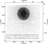 |
Fig. 1 Spatial positions of all detected stars in NGC 1783 field on the ACS/WFC chip. The circle indicates the core radius of the cluster and the center of the cluster is indicated with a (red) asterisk symbol. We used the rectangle, shown at the bottom of the chip, as our reference field region for the statistical removal of field stars from the cluster region. The white line containing no stars is due to the gap between the two detector chips. |
As cluster fields, we selected the areas that are within one to two times the core radii of the clusters. We had to find a compromise for the size: On the one hand we want to chose a region large enough to have as many cluster stars as possible for our analysis while, on the other hand, the region had to be small enough to perform a reasonable field star subtraction, since the distance between the reference and the cluster field is limited. For most of the clusters, we selected an area within two times the core radius Rcore (radius at which the density is half the central density) as our cluster field. We selected the area within one Rcore for NGC 1783 and NGC 2203, which have large core radii (cf. Table 1), and NGC 1987, which has a very numerous underlying field star population.
After defining the cluster and the reference field, we constructed CMDs for both fields. For every star in the reference CMD, we removed the star in the cluster CMD that is closest to the reference field star in color−magnitude space (cf. Niederhofer et al. 2015a). As two examples, Figs. 2 and 3 show the CMDs of all stars in the cluster field of NGC 1783 and Hodge 2 (left panels), the CMDs of the reference field (middle panels), and the field subtracted cluster CMDs (right panels). We note that a rich underlying old population, which has a MSTO at mF475W ~ 22, is present in the CMD of Hodge 2 (Fig. 3 middle panel). This population is not completely subtracted and is still visible in the cleaned CMD (right panel), where it causes the “bump” feature in the MS at mF475W ~ 22. The method of the statistical field star subtraction relies on two assumptions: First, that the field stars are distributed equally over the entire field of view; second, that there are no cluster stars left in the reference field. However, in our case, the second assumption is not entirely fulfilled since we do not have an additional external field exposure for the clusters, but rather performed the decontamination on the cluster exposure itself. The tidal radii Rtidal (the radius at which the gravitational force of the host galaxy becomes larger than that of the cluster itself) of the clusters are at least five times larger than their core radii (Goudfrooij et al. 2011a, 2014), and there are still some cluster stars left in our reference fields. We might also, therefore, subtract cluster stars.
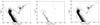 |
Fig. 2 Left panel: CMD of all stars within the core area of NGC 1783; Middle panel: CMD of the selected field star region (rectangular area in Fig. 1); Right panel: CMD of the core area of NGC 1783 decontaminated from the field star population. However, it is not fully decontaminated as there are still some non-cluster stars left in the cleaned CMD. The two gray rectangles indicate the boxes used for fitting the SFH of the turn-off and red clump region. Note that the limits of the boxes are shifted to the non-extinction corrected data. |
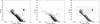 |
Fig. 3 Left panel: CMD of all stars within the core area of Hodge 2, Middle panel: CMD of the selected field star region, Right panel: CMD of the core area of Hodge 2 decontaminated from the field star population. As in Fig. 2, the gray boxes indicate the areas in the CMD where we fit the SFH. |
2.4. Differential extinction correction
Milone et al. (2009) and Goudfrooij et al. (2011a) report in their works that NGC 2108 might be affected by differential extinction. We take this effect into account and correct NGC 2108 for differential reddening before carrying out the analysis. We followed the procedure that is described in Milone et al. (2012b). We recap here only the main steps of the correction: We rotated the CMD of NGC 2108, such that the reddening vector is horizontal. Then we defined a fiducial line in the rotated CMD along the MS well below the TO region by quadratically interpolating the median x-values of the MS stars in the rotated CMD in bins of 0.25 in y-units. For each star on the MS, we calculated the median horizontal displacement from the fiducial line for the closest 10−20 (depending on the spatial position of the star in the cluster) neighbors (not including the star itself). This median displacement, since it is parallel to the extinction vector, is a measure for the local reddening. As a final step, we took the spatial median of the local extinction over a bin size of about 175 × 175 pixel (as a trade-off between spatial resolution and numbers of stars per bin) and corrected each cluster star for its local reddening. We find a differential reddening across the cluster that has a standard deviation of about 0.07 mag in AV with a maximum value of 0.21 mag. Figure 4 shows the CMD of NGC 2108 before (top panel) and after (lower panel) the correction for differential extinction. Although the differences are very moderate, the CMD of NGC 2108 has improved. The main sequence and the turn-off are smoother and better defined. Also the red clump now has a more compact shape. In the further analysis we use the corrected photometry.
3. Models and methods
3.1. Models
In this study we analyze the CMDs of a sample of 12 intermediate-age LMC clusters which all show the extended MSTO phenomenon. Li et al. (2014) and Bastian & Niederhofer (2015) compare the distributions of stars that populate the SGB and the red clump with expected findings for an SSP and an extended SFH. We continue these studies by performing a quantitative study of the SFH of the clusters in our sample. We perform the SFH fitting on two regions of the cluster CMDs, first on the extended main-sequence turn-off, and secondly on the post-main-sequence region that includes the sub-giant branch, lower red giant branch and red clump. For this, we fitted the SFH in the MSTO and post-MS regions, including the SGB and the red clump, independently. For our analysis we used the StarFISH package (Harris & Zaritsky 2001). This code uses theoretical isochrones to create a library of synthetic single age CMDs. It takes the photometric errors of the observations into account and requires an a priori knowledge (or assumption) of the metallicity Z, the distance modulus, and extinction. Below the MSTO, StarFISH linearly interpolates along the isochrones as a result of the sparser sampling. However, the code does not interpolate between isochrones at different ages. To reconstruct the SFH from the observed CMD, the StarFISH code linearly combines the synthetic CMDs and searches for the best match between model and data by performing a χ2 minimization.
As theoretical models for the fitting, we used the newest PARSEC 1.2S isochrones (Bressan et al. 2012) from the Padova isochrone set3 at a fixed metallicity Z of 0.008 (Z⊙ = 0.0152 for this set of isochrones) and a He abundance Y of 0.25. These isochrones are computed from evolutionary tracks with a two times finer mass grid (ΔM = 0.05 M⊙) than the older set of Marigo et al. (2008) from the same group. A metallicity of 0.008 is a typical value of LMC clusters in this age interval. For all the clusters, we fitted the SFH between log(age) = 8.70 and log(age) = 9.50 in steps of 0.03 (in log).
3.2. Isochrone fitting
Parameters of the LMC clusters.
 |
Fig. 4 CMDs of NGC 2108 before and after the correction for differential extinction. Upper panel: the original CMD; lower panel: the corrected CMD. The gray boxes show the areas in the CMD used to fit the SFH of the MSTO and the red clump. The limits have been shifted to match the data that has not been corrected for the mean extinction. |
To determine the basic parameters of the clusters in our sample that are needed to fit the SFH (distance modulus (m−M)0, extinction AV), we fitted theoretical models to the CMDs. To calculate the reddening in each filter from the visual extinction AV, we used the following conversion factors: For the ACS/WFC filter system: AF435W = 1.351 AV, AF555W = 1.026 AV, and AF814W = 0.586 AV (Goudfrooij et al. 2009). And for the WFC3/UVIS filter set: AF475W = 1.192 AV and AF814W = 0.593 AV (Goudfrooij et al. 2014). The filter-dependent extinction conversions were derived using the ACS/WFC and WFC3/UVIS filter curves and a Cardelli et al. (1989) extinction law with RV = 3.1. To determine the best-fit parameters, we selected isochrones with ages of between 500 Myr and 2 Gyr. These were then adjusted by eye for both distance modulus and AV to match the main sequence and the red clump. In most cases the red clump is well defined, which leads to small uncertainties in both parameters. For the younger clusters, however, which have more extended red clumps, there is more uncertainty in both parameters, extinction, and distance modulus. However, our results are not dependent on the exact choice of the parameters since we are interested in the relative differences between the turn-off and the red clump of the same cluster. The values of the reddening AV and distance modulus that were found in this study and used for further analysis can be found in Table 1. We note that we determined the distance moduli of all but two clusters as being less than the canonical distance modulus of the LMC center (18.50 mag  50 kpc). The only exceptions are NGC 1718 and NGC 1806, for which we found a distance modulus of 18.54 mag (51 kpc). Most of the clusters are located well in front of the LMC, up to 3 kpc if the nominal distance to the LMC is adopted. However, we also note that the LMC distance was not derived consistently with the methods used here (i.e., there may be systematic uncertainties that account for the different distances).
Limits of the boxes where the SFH is fitted.
3.3. Fitting of the star-formation history
We used the StarFISH software package for the fitting of the SFH, assuming: i) a Salpeter (1955) initial mass function; ii) the values of AV and (m−M)0 determined in the previous section; iii) a binary fraction of 0.3 for each cluster. Goudfrooij et al. (2014) simulated the CMDs of a sample of 11 intermediate age LMC and SMC clusters leaving the binary fraction as a free parameter. For most of the clusters they found best-fitting values between 0.22 and 0.33. To test how the assumed fraction of binaries affects the results for the SFH, we tried different values of the binary fraction between 0.1 and 0.5 and found that the overall shape of the SFH, both for the MSTO and red clump region, does not change significantly for values between 0.2 and 0.4.
Furthermore, the SFH code requires a model of the photometric errors and the completeness fraction. We have photometric error estimates derived from a series of artificial star tests for the cluster sample from Goudfrooij et al. (2014). For the other clusters we created an analytical model for the photometric errors within StarFISH, based on the following estimates: We assumed a photometric error of 0.01 in the F435W filter for the brightest stars in the clusters, which is comparable to the errors inferred from the artificial star tests. The errors increase exponentially to about 0.03 to 0.045 at F435W magnitudes between 23.5 and 25, depending on the cluster. We estimated the errors from the width of the main sequence (well below the MSTO). From the artificial star tests, we find a 90% completeness limit at a magnitude of between 25 and 23.5 in F475W, depending on the cluster. Only Hodge 2 has a lower 90% completeness limit at about 21.2 mag in F475W because of the high crowding in its field. The limits should be comparable for the clusters from the ACS/WFC sample. However, incompleteness will not significantly affect our analysis as we are interested in the morphology of the MSTO and the red clump, both of which are above the 90% completeness limit in all cases. We tested the reliability of our assumed error model by applying it to a cluster from the Goudfrooij et al. (2014) data set and fitted the SFH of the cluster using the analytical error model again. The similarity of the results suggests that our adopted error model is reasonable.
We fit the SFH in two separate parts of the CMD, one centered on the extended MSTO and one including the red clump, SGB, and lower red giant branch. The limits of the boxes that contain the regions that we used for the fitting are listed in Table 2. We binned the MSTO region into grid boxes that are 0.05 × 0.05 mag in size. For the red clump region, we choose bins that are 0.025 × 0.025 mag. Only for LW 431, which has a very sparsely populated red clump, did we use a bin size of 0.05 × 0.05 mag for the red clump.
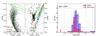 |
Fig. 5 Left panel: CMD of the MSTO and red clump region of NGC 1783 together with overplotted isochrones at three different ages that cover the extent of the MSTO. Right panel: fitted SFH of NGC 1783 using only the MSTO region (blue solid line) and only the red clump region (red dashed line) along with 1σ error bars showing the statistical errors. The error bars result from bootstrapping the data (see text for details). |
4. Results
4.1. The star-formation history of the main-sequence turn-off and the red clump
The left panels of Figs. 5, 6 and B.1 to B.10 show the CMDs of each cluster in our sample, zoomed into two regions: The left of the two CMDs is centered at the turn-off region, and the right one is centered around the red clump. Additionally, for every cluster we show the best-fitting isochrones at three ages that span the extent of their turn-offs. The ages of the isochrones are given in the CMD that shows the red clump. The parameters used to transform the isochrones from the absolute magnitude plane to the apparent magnitude plane (visual extinction, distance modulus) are stated in the lower left corner of the main sequence CMD. The typical age spreads of the isochrones describing the extended MSTO are approximately 400 to 500 Myr. The same isochrones are also shown in the plots showing the red clumps of the clusters. By making a visual comparison, we see that the red clumps of most of the clusters are compact in shape. However, it seems that some are not in agreement with a single age, and especially those clusters that have ages of around 1.7 Gyr show an extension towards lower luminosities in their red clumps. These stars follow a younger isochrone. For the younger clusters (e.g. NGC 1987 and NGC 2108) the isochrones of between ~800 Myr and ~1.2 Gyr coincide at the position of the red clump. Also NGC 2108 has a red clump which is quite extended in color. This might be a consequence of a remaining component of the differential reddening that was not removed completely.
The right panels of Figs. 5, 6 and B.1 to B.10 show the results of the SFH fitting. The blue histograms (blue solid line) correspond to the SFH of the MSTO region. The red histograms (red dashed line) show the age distribution inferred from the red clump region. All SFH plots show the expected statistical errors on the fitting, which we estimated from using a series of bootstrapping. We created 20 bootstrap realizations for each cluster and fitted their SFH. The histograms show the mean of the results, along with the 1σ error bars.
For most of the clusters in our sample, we find that the age spread that results from the red clump region is smaller than the one from the MSTO. However, the red clumps of all but two clusters are not in agreement with a single age. The post main sequence age distributions of LW 431, NGC 2203, NGC 1651, NGC 2213, NGC 2173, and NGC 1846 are narrower, relative to the ones inferred from the width of the MSTO. The red clumps of NGC 1783, Hodge 2, NGC 2108, and NGC 1806 show an extent which is comparable to the age spread of the MSTO. As we already pointed out, NGC 2108 is affected by differential extinction. In Sect. 2.4, we corrected the CMD for this effect, however, there is the possibility that it was not removed completely. Therefore, some remaining variation in reddening across the cluster might introduce some scatter in the SFH of this cluster. This might also be the cause for the low level of fitted star formation at higher ages. Only NGC 1718 and NGC 1987 show a single peak of star formation in the red clump, i.e., it seems to be consistent with a single isochrone. In Table 1 we summarize the ages and the maximum age spreads of the clusters inferred from the fitted SFH of the red clumps.
To assess the reliability of the fitted SFH, we created two artificial clusters for each cluster in our sample, one with the fitted SFH from the MSTO, and one with the age distribution inferred from the red clump region. For this we made use of the function repop within StarFISH. The clusters were created with the same parameters that we used to fit the SFH. Also we normalized the number of stars to be the same in both the observed and the synthetic clusters. In Appendix A (Fig. A.1) we present the CMDs of all artificial clusters that were created. The two upper panels of each subplot show the clusters created from the fitted SFH of the red clump region, whereas the lower two panels display the artificial clusters using the recovered SFH from the MSTO. The CMDs have the same limits as the CMDs of their real counterparts, shown in Figs. 5, 6 and B.1 to B.10, and the overlaid isochrones are also the same to make a better comparison. The ages of the isochrones are given in the lower right panel of each cluster’s subplot. For the majority of clusters, we see that the reconstructed MSTO and red clump from the fitted SFH of the respective CMD region are both in good agreement with the observations (see upper right and lower left panel of each subplot in Fig. A.1). The fact that the extended MSTO in the simulations has no smooth structure but shows distinct peaks is due to our finite age resolution in the fitting (log(Δage) = 0.3) and the fact that StarFISH does not interpolate between isochrones. Each peak corresponds to an individual value in the histogram of the fitted SFH.
We also note that, in clusters like NGC 1987, NGC 1718, NGC 2203, or NGC 1846, the MSTO resulting from the red clump fit is narrower than the observed ones and more concentrated. The red clumps in clusters like NGC 1783 or NGC 1806 are more compact, as would be expected from the fitted SFH. This suggests that the fit overestimates the range of ages present in these clusters. By comparing the CMDs of the two younger clusters, Hodge 2 and NGC 2108, with the artificial clusters, it is noticeable that the reconstructed SFH of the red clump region is a poor fit to the observed data. Therefore, these last two clusters do not provide any meaningful contribution to our overall results.
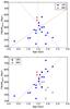 |
Fig. 7 Upper panel: FWHM of the turn-off of clusters in the Goudfrooij et al. (2014) sample as a function of their age. In this plot we also include the 300 Myr-old cluster NGC 1856, which also shows an extended MSTO. Clusters in the LMC are marked with blue circles, whereas the two SMC clusters are denoted with a red asterisk. The width of the MSTO seems to increase with the age of the cluster until an age of 1.5−1.7 Gyr and then decreases again. We divided the plot at 1.5 Gyr (vertical solid gray line) in two parts and performed a linear regression fit to the clusters in the two parts, separately. The fits are indicated by the red dashed line (younger clusters) and the blue dash-dotted line (older clusters). Lower panel: same as the upper panel, but now we mirrored the older clusters at the horizontal plain that goes through the intersection point between the two liner regression fits in the upper panel. We did this to quantify the strength of the correlation of the FWHM with age. The original positions of the clusters are marked with black open circles. The red dashed line is a linear regression fit to the linearized cluster sample. |
5. Correlations with age
Goudfrooij et al. (2014) studied the MSTO of a sample of 18 intermediate-age LMC and SMC clusters in detail. Based on observed properties of the clusters, they found that there is a correlation between the mass of the clusters and the width of the MSTO, in terms of the full width at half maximum (FWHM). Moreover, the correlation becomes even clearer, when the early mass of the clusters is used. Goudfrooij et al. (2014) assume that the clusters underwent strong mass loss in the past and calculate the early masses of the clusters using correction factors that are a strong function of age. The existence of a correlation between the FWHM and “corrected” initial mass of the clusters led Goudfrooij et al. (2014) to conclude that a physical property of the cluster (i.e., mass or escape velocity) was the determinant as to whether clusters could host extended star-formation events.
Here we look for additional correlations, such as the age of the clusters. For this we took the values of the age and the FWHM of the clusters’ turn-off as they were given in Goudfrooij et al. (2014), and plotted the FWHM as a function of cluster age (see Fig. 7, upper panel). In this plot we also included the 300 Myr-old cluster NGC 1856 that also shows an extended turn-off (see Sect. 6 for more detail). The turn-off width seems to be correlated with the cluster age in the sense that it first increases as the clusters get older, until an age of 1.5−1.7 Gyr. Then the extent of the MSTO decreases again. Such a behavior is to be expected if stellar rotation causes the spread in the MSTO (Brandt & Huang 2015a; Niederhofer et al. 2015b). However, there are two outliers to this relation, NGC 1795 at 1.4 Gyr and IC 2146 at 1.9 Gyr, which both have a compact MSTO structure. Goudfrooij et al. (2014) additionally included these two low-mass clusters from the sample of Milone et al. (2009) in their mass vs. FWHM relation.
We now divide the diagram into two parts at 1.5 Gyr and have a closer look at the “young” and “old” branches separately (we note that the general result does not depend on the exact choice of the age at which we divide the data). To quantify the correlation, we follow the procedure described in Goudfrooij et al. (2014) and also performed a Kendall τ test for both of the branches. We performed this test two times, once excluding the outliers NGC 1795 and IC 2146, and once including them. The values in parenthesis give the results without the two clusters. We found that the two-sided τ value is 0.59 (0.82) for the younger clusters and −0.6 (−0.6) for the older clusters. The pτ value of the test, which gives the probability that the values are uncorrelated, is 2.7% (0.5%) for the increasing branch and 0.7% (1.0%) for the decreasing one. For the FWHM vs. early cluster mass relation, Goudfrooij et al. (2014) found a τ of 0.82 and a pτ of 1%, and for the FWHM vs. early escape velocity relation they obtained a τ value of 0.98 and a pτ of 0.2%.
To quantify the strength of the overall correlation, we turned the Λ shaped function into a monotonically increasing function by mirroring the older clusters at the vertical line that goes through the intersection point of the two linear fits. This “linearized” function is shown in the lower panel of Fig. 7. The original positions of the older clusters in the diagram are indicated by black open circles. The red dashed line is a linear regression fit to the linearized data. We then performed another Kendall τ test to the entire data. Here too, the values in parenthesis give the results which exclude NGC 1795 and IC 2146. The Kendall τ value is now 0.65 (0.65) and the pτ value gives a probability of 0.004% (0.009%) that a correlation is absent in the data. In terms of the scenario proposed by Goudfrooij et al. (2014), where the width of the MSTO is caused by an age spread, this kind of correlation with age would not be expected. Although the Kendall τ test, which is not very sensitive to single outliers, suggests that there is a strong correlation between the FWHM and the age of the clusters, there are clusters that do not follow this relation. There is also the possibility that the found Λ shaped curve is an envelope that gives an upper limit to the FWHM as a function of age. We note that in the stellar rotation scenario, the width of the MSTO depends on the rotation distribution within the cluster, which may vary between clusters.
6. Discussion and conclusions
In this study, we have analyzed the CMDs of a sample of 12 intermediate-age LMC clusters which all show an extended MSTO. We have fitted the SFH in two portions of the CMD, a) centered on the extended MSTO and b) focused on the red clump, SGB, and lower red giant branch.
To reconstruct the SFH of the 12 clusters in our sample, we made use of the PARSEC 1.2S isochrone set. Our main result shows that, for ten out of 12 clusters, the fitted SFH inferred from the red clump region is not compatible with the range of stellar ages that result from the MSTO, but it is narrower. However, the red clumps also show an extended SFH and are not in agreement with a coeval stellar population. Only in NGC 1806 (and to a lesser extent NGC 1783) are the inferred SFHs derived from the red clump and MSTO region comparable. However, as can be seen in Fig. A.1, the observed red clump has a more compact structure than would be expected from the fitted SFH, suggesting that we over-estimated its age spread. We also found that for most of the clusters, the peak of the reconstructed red clump and MSTO ages coincide. There are two exceptions to this, Hodge 2 and NGC 2108. In the first cluster, we find an additional peak in the red clump SFH that has no counterpart in the MSTO. In the second one, NGC 2108, the age distribution of the red clump shows two peaks, one on each side of the peak of the MSTO SFH.
The results that we obtained in this work differ from the findings by Li et al. (2014) and Bastian & Niederhofer (2015). These studies analyzed the morphology of the SGB and the red clump of NGC 1651, NGC 1806, and NGC 1846 and compared it to expected findings if the MSTO was due to an age spread. Both studies adopted the Marigo et al. (2008) isochrones. They concluded that: a) SGB and red clump position and morphology were not consistent with the inferred age spreads from the MSTO; and b) the SGB and the red clump follow the youngest isochrone going through the turn-off. However, our findings, which are based on the PARSEC isochrone set, on the one hand suggest that the red clump in these cluster is more extended than would be expected from a single age and, on the other hand, that the peak age of the red clump and MSTO agree with each other.
The results are in line with the recent study by Goudfrooij et al. (2015), in which the analysis of the MSTO is coupled with the study of the SGB morphology in the clusters NGC 1651, NGC 1783, NGC 1806, and NGC 1846. In contrast to the studies by Li et al. (2014) and Bastian & Niederhofer (2015), they argue that the position of the SGB should not be used (because of uncertainties in the stellar models) but rather that the width is a better indicator of age spreads. The authors find that the width of the SGB of these clusters does agree with an extended SFH using the Marigo et al. (2008) set of isochrones. However, Li et al. (in prep.) find that the width of the SGB of NGC 411 is significantly lower than expected from the MSTO width, if an age spread is present.
Additionally, Goudfrooij et al. (2015) studied the red clump of NGC 1806 using a finer mass resolution (ΔM = 0.01 M⊙) grid of PARSEC isochrones. The authors find that the red clump is more extended than expected for a single age population, with a width similar to that found from the MSTO. This agrees with the results presented here. Goudfrooij et al. (2015) also highlighted an elongated extension that lies below the otherwise compact red clump. This additional “tail” was interpreted as a “double red clump”, similar to that found in the SMC clusters NGC 411 and NGC 419 (Girardi et al. 2009 and Girardi et al. 2013). These stars are believed to be slightly more massive, and therefore younger stars that are just massive enough to avoid the state of degenerate core He-burning. Overall, our results agree with the findings by Goudfrooij et al. (2015) in terms of the range of ages in the red clump is extended and not compatible with a coeval population. However, our fitting of the SFH suggests that the age spread in the red clump, in most clusters in our sample, is smaller than what would be expected from the MSTO. We also note that stellar rotation is expected to broaden the red clump to some degree.
In conclusion, the results we found in this work are ambiguous and neither confirm nor exclude large age spreads in intermediate-age LMC clusters. Owing to the uncertainties in the stellar models, especially at post-MS phases, an analysis of the CMDs of extended MSTO clusters alone seems insufficient to test the nature of the extended MSTO. For this reason, independent and complementary observations should be used to test whether age spreads are present within massive clusters. A variety of observations already exist that are at odds with the predictions of an age spread scenario. In the following we list the arguments that disfavour an age spread as the cause of the extended MSTO regions.
6.1. Other considerations on age spreads within clusters
If age spreads are present in these intermediate-age LMC clusters then, as a consequence, young clusters with similar properties should have age spreads or signs of star formation as well. However, no evidence of ongoing star formation has been found in young massive clusters in the LMC and other galaxies (e.g., Bastian et al. 2013b; Cabrera-Ziri et al. 2014). Bastian & Silva-Villa (2013) and Niederhofer et al. (2015a) found no evidence for age spreads comparable in duration to that suggested for the intermediate-age clusters in a sample of 14 young massive LMC clusters. There could be some spreads present in the young clusters (the case of NGC 1856 will be discussed in more detail below), however these spreads would be much smaller that those inferred for the intermediate-age clusters, and the spread is a function of cluster age (Niederhofer et al. 2015b).
Also, the formation of a second generation of stars requires a gas reservoir inside the clusters out of which the new stars can be formed. Several studies have searched for gas inside young and massive clusters and up to now none have been found (e.g., Bastian & Strader 2014; Cabrera-Ziri et al. 2015; see also Longmore 2015). Bastian et al. (2014) and Hollyhead et al. (2015) showed that young massive clusters expel their gas to over 200 pc in just a few Myr. It is not clear how this gas should be reaccreted to the cluster again.
Goudfrooij et al. (2014) found a correlation between the width of the MSTO and the escape velocity of the cluster at young ages after applying large correction factors to the current values. To calculate these early escape velocities, Goudfrooij et al. (2014) adopt the models by D’Ercole et al. (2008) which were designed for highly extended and tidally limited clusters within a strong tidal field. However, it is not clear if such models could be applied in the LMC and SMC, as the the tidal field (especially for the SMC clusters that are far out in the galaxy) in these galaxies is much weaker than in the inner regions of the Milky Way, where the original models were applied. Goudfrooij et al. (2014) concluded that there is a velocity threshold beyond which the cluster is able to retain the slow wind ejecta of evolved stars to form a second generation of stars inside the cluster. They determined this threshold is at 12−15 km s-1. In the model of Goudfrooij et al. (2014) the clusters are expected to have been three to four times more massive in the past. But the clusters appear to be well contained within their tidal radii (Glatt et al. 2011), so their mass loss is expected to be very low, unless their current positions have only recently been acquired.
Finally, if age spreads were present in the clusters and if the second generation of stars were formed (at least partially) out of the ejecta of AGB stars, then chemical abundance spread would be expected inside the cluster. However, Mucciarelli et al. (2008, 2011, 2014) analyzed the extended MSTO clusters NGC 1651, NGC 1783, NGC 1806, NGC 1846, and NGC 2173 and did not find evidence for significant abundance spreads.
6.2. An alternative explanation
As an alternative scenario to age spreads, Bastian & de Mink (2009) propose the idea that the broadening of the MSTO could be caused by rotating stars. However, their results are disputed by Girardi et al. (2011). Later, Yang et al. (2013) show in their study that a MSTO broadening could indeed be expected for stellar rotation at the ages of the extended MSTO clusters. The models of Yang et al. (2013) predict that the turn-off of rotating stars is redder and fainter for ages between 0.8 and 2.2 Gyr and they, therefore, appear older than non-rotating stars. This effect, however, reverses at ages older than about 2.4 Gyr, where rotating MSTO stars are bluer and brighter than their non-rotating counterparts. Whereas stellar rotation seems to be able to broaden the turn-off region in the way it is observed, it is not clear how it affects the SGB and the red clump.
Brandt & Huang (2015a) use the syclist rotating stellar models (Georgy et al. 2013) to compute synthetic photometry of stars of varying rotation rates. They were able to reproduce the extended MSTO features in clusters between one and two Gyr with stars at different rotation velocities and viewing angles. Also, Brandt & Huang (2015b) analyze the two younger (800 Myr) nearby Hyades and Praesepe open clusters. Both clusters show an extended MSTO feature that does not seem to be in agreement with a coeval population (e.g., Eggen 1998). Because the clusters only have stellar masses of ~400 M⊙ (Hyades, Perryman et al. 1998) and ~500 M⊙ (Praesepe, Kraus & Hillenbrand 2007), they do not fit the Goudfrooij et al. (2014) scenario. Piatti & Bastian (2015) find extended main sequences in a sample of four low-mass intermediate-age LMC clusters (<5000 M⊙), suggesting that cluster mass does not determine whether a cluster can host an extended MSTO.
Brandt & Huang (2015b) show that the spread at the turn-off can be explained with stellar rotation without the need of a prolonged SFH. Similarly, Niederhofer et al. (2015b) compare rotating and non-rotating isochrones from the syclist models. They find that stars which rotate at different velocities in a coeval population can produce an extended MSTO feature. The predicted spread in the turn-off is proportional to the age of the cluster and seems to follow the observations closely.
6.3. Young clusters
There might also be other effects present in the CMDs of clusters that do not agree with an SSP and which we do not completely understand. Milone et al. (2013b) study the young (~150 Myr) moderately massive (5.0 × 10³M⊙, Baumgardt et al. 2013) cluster NGC 1844 in the LMC using HST photometry. The main sequence of this cluster shows broadened features which are shown to be an intrinsic property of the cluster. The authors try to explain the broadening using various approaches, including stellar rotation and multiple populations, including both different ages and spreads in metallicity, He content, and C-N-O abundance. While Milone et al. (2013b) exclude multiple stellar populations as causing the broadened main sequence, other explanations, like stellar rotation, also yield unsatisfying results in their simple approach. This work shows that there are still observations of CMDs that are currently not reproduced well by stellar models.
Milone et al. (2015) and Correnti et al. (2015) find evidence that NGC 1856, which is only 300 Myr-old, has an extended MSTO, as well. This is the first detection of a broadened turn-off in a cluster younger than 1 Gyr. The studies found that the width of the turn-off would correspond to an age spread of 180 Myr (Correnti et al. 2015) or 150 Myr (Milone et al. 2015). Additionally, Milone et al. (2015) have discovered that the main sequence of NGC 1856 splits into two parts beneath the turn-off, which could be due to a spread in age or to chemical abundance variations. D’Antona et al. (2015) analyze the CMD of NGC 1856 concentrating on the split of the main-sequence and the extended turn-off region. They find that these features can also be explained with a rapidly rotating and a non-rotating population, with both having the same age. These detections also provide evidence that young clusters are not SSPs, even though their deviations are smaller than those from intermediate-age clusters. Therefore, it is tempting to claim that whatever causes this anomaly, changes with the age of the cluster.
6.4. Summary
Taking all the facts together, it is still unclear what causes the extended MSTO. With 8-10m class ground-based facilities, it will be possible to test the rotating stars scenario and measure the projected rotation velocity vsin(i) of stars directly along the spread of the MSTO. These measurements will give a definitive answer as to how much rotating stars contribute to the spread in color and magnitude at the end of their main-sequence lifetime.
IRAF is distributed by the National Optical Astronomy Observatories, which is operated by the Association of Universities for Research in Astronomy, Inc., under cooperative agreement with the National Science Foundation.
Acknowledgments
We are grateful to Paul Goudfrooij and Antonino Milone for providing their photometry and catalogs. We thank the anonymous referee for useful comments and suggestions that helped us to improve the manuscript. We thank Aaron Dotter for his useful comments. This research was supported by the DFG cluster of excellence “Origin and Structure of the Universe”. N.B. is partially funded by a Royal Society University Research Fellowship. V.K.-P. is greatly appreciative to Jay Anderson for sharing with us his ePSF library PSF fitting software. Support for this work was provided by NASA through grant number AR-12642 from the Space Telescope Science Institute, which is operated by AURA, Inc., under NASA contract NAS 5-26555.
References
- Anderson, J., & Bedin, L. R. 2010, PASP, 122, 1035 [NASA ADS] [CrossRef] [Google Scholar]
- Anderson, J., & King, I. R. 2006, PSFs, Photometry, and Astrometry for the ACS/WFC, ACS Instrument Science Report 2006-01 (Baltimore, MD: STScI) [Google Scholar]
- Bastian, N., & de Mink, S. E. 2009, MNRAS, 398, L11 [NASA ADS] [CrossRef] [Google Scholar]
- Bastian, N., & Niederhofer, F. 2015, MNRAS, 448, 1863 [NASA ADS] [CrossRef] [Google Scholar]
- Bastian, N., & Silva-Villa, E. 2013, MNRAS, 431, 122 [Google Scholar]
- Bastian, N., & Strader, J. 2014, MNRAS, 443, 3594 [NASA ADS] [CrossRef] [Google Scholar]
- Bastian, N., Lamers, H. J. G. L. M., de Mink, S. E., et al. 2013a, MNRAS, 436, 2398 [NASA ADS] [CrossRef] [MathSciNet] [Google Scholar]
- Bastian, N., Cabrera-Ziri, I., Davies, B., & Larsen, S. S. 2013b, MNRAS, 436, 2852 [Google Scholar]
- Bastian, N., Hollyhead, K., & Cabrera-Ziri, I. 2014, MNRAS, 445, 378 [NASA ADS] [CrossRef] [Google Scholar]
- Bastian, N., Cabrera-Ziri, I., Salaris, M. 2015, MNRAS, 449, 3333 [NASA ADS] [CrossRef] [Google Scholar]
- Baumgardt, H., Parmentier, G., Anders, P., & Grebel, E. K. 2013, MNRAS, 430, 676 [NASA ADS] [CrossRef] [Google Scholar]
- Brandt, T. D., & Huang, C. X. 2015a, ApJ, 807, 25 [NASA ADS] [CrossRef] [Google Scholar]
- Brandt, T. D., & Huang, C. X. 2015b, ApJ, 807, 24 [NASA ADS] [CrossRef] [Google Scholar]
- Bressan, A., Marigo, P., Girardi, L., et al. 2012, MNRAS, 427, 127 [NASA ADS] [CrossRef] [Google Scholar]
- Cabrera-Ziri, I., Bastian, N., Davies, B., et al. 2014, MNRAS, 441, 2754 [NASA ADS] [CrossRef] [Google Scholar]
- Cabrera-Ziri, I., Bastian, N., Longmore, S. N., et al. 2015, MNRAS, 448, 2224 [NASA ADS] [CrossRef] [Google Scholar]
- Cardelli, J. A., Clayton, G. C., & Mathis, J. S. 1989, ApJ, 345, 245 [NASA ADS] [CrossRef] [Google Scholar]
- Conroy, C., & Spergel, D. N. 2011, ApJ, 726, 36 [NASA ADS] [CrossRef] [Google Scholar]
- Correnti, M., Goudfrooij, P., Kalirai, J. S., et al. 2014, ApJ, 793, 121 [NASA ADS] [CrossRef] [Google Scholar]
- Correnti, M., Goudfrooij, P., Puzia, T. H., & de Mink, S. E. 2015, MNRAS, 450, 3054 [NASA ADS] [CrossRef] [Google Scholar]
- D’Antona, F., Di Criscienzo, M., Decressin, T., et al. 2015, MNRAS, 453, 2637 [NASA ADS] [Google Scholar]
- Decressin, T., Charbonnel, C., Siess, L., et al. 2009,A&A, 505, 727 [Google Scholar]
- de Mink, S. E., Pols, O. R., Langer, N., & Izzard, R. G. 2009, A&A, 507, L1 [NASA ADS] [CrossRef] [EDP Sciences] [Google Scholar]
- D’Ercole, A., Vesperini, E., D’Antona, F., McMillan, S. L. W., & Recchi, S. 2008, MNRAS, 391, 825 [NASA ADS] [CrossRef] [Google Scholar]
- Eggen, O. J. 1998, AJ, 116, 284 [NASA ADS] [CrossRef] [Google Scholar]
- Georgy, C., Ekström, S., Eggenberger, P., et al. 2013, A&A, 558, A103 [NASA ADS] [CrossRef] [EDP Sciences] [Google Scholar]
- Girardi, L., Rubele, S., & Kerber, L. 2009, MNRAS, 394, L74 [NASA ADS] [Google Scholar]
- Girardi, L., Eggenberger, P., & Miglio, A. 2011, MNRAS, 412, L103 [NASA ADS] [Google Scholar]
- Girardi, L., Goudfrooij, P., & Kalirai, J. S. 2013, MNRAS, 431, 3501 [NASA ADS] [CrossRef] [Google Scholar]
- Glatt, K., Grebel, E. K., Jordi, K., et al. 2011, AJ, 142, 36 [NASA ADS] [CrossRef] [Google Scholar]
- Goudfrooij, P., Puzia, T. H., Kozhurina-Platais, V., & Chandar, R. 2009, AJ, 137, 4988 [NASA ADS] [CrossRef] [Google Scholar]
- Goudfrooij, P., Puzia, T. H., Kozhurina-Platais, V., & Chandar, R. 2011a, ApJ, 737, 3 [NASA ADS] [CrossRef] [Google Scholar]
- Goudfrooij, P., Puzia, T. H., Chandar, R., & Kozhurina-Platais, V. 2011b, ApJ, 737, 4 [NASA ADS] [CrossRef] [Google Scholar]
- Goudfrooij, P., Girardi, L., Kozhurina-Platais, V., et al. 2014, ApJ, 797, 35 [NASA ADS] [CrossRef] [Google Scholar]
- Goudfrooij, P., Girardi, L., Rosenfield, P., et al. 2015, MNRAS, 450, 1693 [NASA ADS] [CrossRef] [Google Scholar]
- Gratton, R. G., Carretta, E., & Bragaglia, A. 2012, A&ARv, 20, 50 [CrossRef] [Google Scholar]
- Harris, J., & Zaritsky, D. 2001, ApJS, 136, 25 [NASA ADS] [CrossRef] [Google Scholar]
- Hollyhead, K., Bastian, N., Adamo, A., et al. 2015, MNRAS, 449, 1106 [NASA ADS] [CrossRef] [Google Scholar]
- Kraus, A. L., & Hillenbrand, L. A. 2007, AJ, 134, 2340 [NASA ADS] [CrossRef] [Google Scholar]
- Larsen, S. S., Strader, J., & Brodie, J. P. 2012, A&A, 544, A14 [Google Scholar]
- Li, C., de Grijs, R., & Deng, L. 2014, Nature, 516, 367 [NASA ADS] [CrossRef] [Google Scholar]
- Longmore, S. N. 2015,MNRAS, 448, L62 [Google Scholar]
- Mackey, A. D., & Broby Nielsen, P. 2007, MNRAS, 379, 151 [NASA ADS] [CrossRef] [Google Scholar]
- Mackey, A. D., Broby Nielsen, P., Ferguson, A. M. N., & Richardson, J. C. 2008, ApJ, 681, L17 [NASA ADS] [CrossRef] [Google Scholar]
- Marigo, P., Girardi, L., Bressan, A., et al. 2008, A&A, 482, 883 [NASA ADS] [CrossRef] [EDP Sciences] [Google Scholar]
- Milone, A. P., Bedin, L. R., Piotto, G., & Anderson, J. 2009, A&A, 497, 755 [NASA ADS] [CrossRef] [EDP Sciences] [Google Scholar]
- Milone, A. P., Marino, A. F., Piotto, G., et al. 2012a, ApJ, 745, 27 [NASA ADS] [CrossRef] [Google Scholar]
- Milone, A. P., Piotto, G., Bedin, L. R., et al. 2012b, A&A, 540, A16 [NASA ADS] [CrossRef] [EDP Sciences] [Google Scholar]
- Milone, A. P., Marino, A. F., Piotto, G., et al. 2013a, ApJ, 767, 120 [NASA ADS] [CrossRef] [Google Scholar]
- Milone, A. P., Bedin, L. R., Cassisi, S., et al. 2013b, A&A, 555, A143 [NASA ADS] [CrossRef] [EDP Sciences] [Google Scholar]
- Milone, A. P., Bedin, L. R., Piotto, G, et al. 2015, MNRAS, 450, 3750 [NASA ADS] [CrossRef] [Google Scholar]
- Mucciarelli, A., Carretta, E., Origlia, L., & Ferraro, F. R. 2008, AJ, 136, 375 [NASA ADS] [CrossRef] [Google Scholar]
- Mucciarelli, A., Cristallo, S., Brocato, E., et al. 2011, MNRAS, 413, 837 [NASA ADS] [CrossRef] [Google Scholar]
- Mucciarelli, A., Dalessandro, E., Ferraro, F. R., Origlia, L., & Lanzoni, B. 2014, ApJ, 793, 6 [Google Scholar]
- Niederhofer, F., Hilker, M., Bastian, N., & Silva-Villa, E. 2015a, A&A, 575, A62 [NASA ADS] [CrossRef] [EDP Sciences] [Google Scholar]
- Niederhofer, F., Georgy, C., Bastian, N., & Ekström, S. 2015b, MNRAS, 453, 2070 [NASA ADS] [CrossRef] [Google Scholar]
- Peacock, M. B., Zepf, S. E., & Finzell, T. 2013, ApJ, 769, 126 [NASA ADS] [CrossRef] [Google Scholar]
- Perryman, M. A. C., Brown, A. G. A., Lebreton, Y., et al. 1998, A&A, 331, 81 [NASA ADS] [Google Scholar]
- Piatti, A. E. 2013, MNRAS, 430, 2358 [NASA ADS] [CrossRef] [Google Scholar]
- Piatti, A. E., & Bastian, N. 2015, MNRAS, submitted [Google Scholar]
- Pinsonneault, M. H., Kawaler, S. D., Sofia, S., & Demarque, P. 1989, ApJ, 338, 424 [NASA ADS] [CrossRef] [Google Scholar]
- Piotto, G., Milone, A. P., Anderson, J., et al. 2012, ApJ, 760, 39 [NASA ADS] [CrossRef] [Google Scholar]
- Rubele, S., Girardi, L., Kozhurina-Platais, V., et al. 2013, MNRAS, 430, 2774 [NASA ADS] [CrossRef] [Google Scholar]
- Salpeter, E. E. 1955, ApJ, 121, 161 [Google Scholar]
- Sirianni, M., Jee, M. J., Benítez, N., et al. 2005, PASP, 117, 1049 [NASA ADS] [CrossRef] [Google Scholar]
- Yang, W. M., & Bi, S. L. 2007, ApJ, 658, L67 [NASA ADS] [CrossRef] [Google Scholar]
- Yang, W., Bi, S., Meng, X., & Liu, Z. 2013, ApJ, 776, 112 [NASA ADS] [CrossRef] [Google Scholar]
Appendix A: Artificial clusters
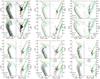 |
Fig. A.1 CMDs of artificial clusters constructed from the fitted SFHs of our sample of LMC clusters. The upper two panels of each subplot show clusters created out of the fitted SFH of the red clump region, whereas the lower panels are synthetic clusters with the recovered SFH from the MSTO region. All CMDs have the same limits as the CMDs of the real counterparts shown in Figs. 5, 6 and B.1 to B.10. The superimposed isochrones are also the same. |
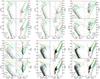 |
Fig. A.1 continued. |
Appendix B: Additional figures
All Tables
All Figures
|
Fig. 1 Spatial positions of all detected stars in NGC 1783 field on the ACS/WFC chip. The circle indicates the core radius of the cluster and the center of the cluster is indicated with a (red) asterisk symbol. We used the rectangle, shown at the bottom of the chip, as our reference field region for the statistical removal of field stars from the cluster region. The white line containing no stars is due to the gap between the two detector chips. |
| In the text | |
|
Fig. 2 Left panel: CMD of all stars within the core area of NGC 1783; Middle panel: CMD of the selected field star region (rectangular area in Fig. 1); Right panel: CMD of the core area of NGC 1783 decontaminated from the field star population. However, it is not fully decontaminated as there are still some non-cluster stars left in the cleaned CMD. The two gray rectangles indicate the boxes used for fitting the SFH of the turn-off and red clump region. Note that the limits of the boxes are shifted to the non-extinction corrected data. |
| In the text | |
|
Fig. 3 Left panel: CMD of all stars within the core area of Hodge 2, Middle panel: CMD of the selected field star region, Right panel: CMD of the core area of Hodge 2 decontaminated from the field star population. As in Fig. 2, the gray boxes indicate the areas in the CMD where we fit the SFH. |
| In the text | |
|
Fig. 4 CMDs of NGC 2108 before and after the correction for differential extinction. Upper panel: the original CMD; lower panel: the corrected CMD. The gray boxes show the areas in the CMD used to fit the SFH of the MSTO and the red clump. The limits have been shifted to match the data that has not been corrected for the mean extinction. |
| In the text | |
|
Fig. 5 Left panel: CMD of the MSTO and red clump region of NGC 1783 together with overplotted isochrones at three different ages that cover the extent of the MSTO. Right panel: fitted SFH of NGC 1783 using only the MSTO region (blue solid line) and only the red clump region (red dashed line) along with 1σ error bars showing the statistical errors. The error bars result from bootstrapping the data (see text for details). |
| In the text | |
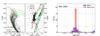 |
Fig. 6 Same as Fig. 5, now for NGC 1846. |
| In the text | |
|
Fig. 7 Upper panel: FWHM of the turn-off of clusters in the Goudfrooij et al. (2014) sample as a function of their age. In this plot we also include the 300 Myr-old cluster NGC 1856, which also shows an extended MSTO. Clusters in the LMC are marked with blue circles, whereas the two SMC clusters are denoted with a red asterisk. The width of the MSTO seems to increase with the age of the cluster until an age of 1.5−1.7 Gyr and then decreases again. We divided the plot at 1.5 Gyr (vertical solid gray line) in two parts and performed a linear regression fit to the clusters in the two parts, separately. The fits are indicated by the red dashed line (younger clusters) and the blue dash-dotted line (older clusters). Lower panel: same as the upper panel, but now we mirrored the older clusters at the horizontal plain that goes through the intersection point between the two liner regression fits in the upper panel. We did this to quantify the strength of the correlation of the FWHM with age. The original positions of the clusters are marked with black open circles. The red dashed line is a linear regression fit to the linearized cluster sample. |
| In the text | |
|
Fig. A.1 CMDs of artificial clusters constructed from the fitted SFHs of our sample of LMC clusters. The upper two panels of each subplot show clusters created out of the fitted SFH of the red clump region, whereas the lower panels are synthetic clusters with the recovered SFH from the MSTO region. All CMDs have the same limits as the CMDs of the real counterparts shown in Figs. 5, 6 and B.1 to B.10. The superimposed isochrones are also the same. |
| In the text | |
|
Fig. A.1 continued. |
| In the text | |
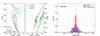 |
Fig. B.1 Same as Fig. 5, now for LW 431. |
| In the text | |
 |
Fig. B.2 Same as Fig. 5, now for NGC 1987. |
| In the text | |
 |
Fig. B.3 Same as Fig. 5, now for NGC 2203. |
| In the text | |
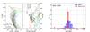 |
Fig. B.4 Same as Fig. 5, now for NGC 1718. |
| In the text | |
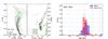 |
Fig. B.5 Same as Fig. 5, now for NGC 1651. |
| In the text | |
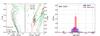 |
Fig. B.6 Same as Fig. 5, now for NGC 2213. |
| In the text | |
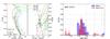 |
Fig. B.7 Same as Fig. 5, now for NGC 2173. |
| In the text | |
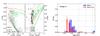 |
Fig. B.8 Same as Fig. 5, now for Hodge 2. |
| In the text | |
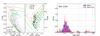 |
Fig. B.9 Same as Fig. 5, now for NGC 2108. |
| In the text | |
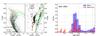 |
Fig. B.10 Same as Fig. 5, now for NGC 1806. |
| In the text | |
Current usage metrics show cumulative count of Article Views (full-text article views including HTML views, PDF and ePub downloads, according to the available data) and Abstracts Views on Vision4Press platform.
Data correspond to usage on the plateform after 2015. The current usage metrics is available 48-96 hours after online publication and is updated daily on week days.
Initial download of the metrics may take a while.