| Issue |
A&A
Volume 586, February 2016
|
|
|---|---|---|
| Article Number | A111 | |
| Number of page(s) | 16 | |
| Section | Astrophysical processes | |
| DOI | https://doi.org/10.1051/0004-6361/201526137 | |
| Published online | 02 February 2016 | |
Shock structures of astrospheres
1 Institut für Theoretische Physik IV: Weltraum- und Astrophysik, Ruhr-Universität Bochum, 44780 Bochum, Germany
e-mail: This email address is being protected from spambots. You need JavaScript enabled to view it.
; This email address is being protected from spambots. You need JavaScript enabled to view it.
2 Research Department, Plasmas with Complex Interactions, Ruhr-Universität Bochum, 44780 Bochum, Germany
e-mail: This email address is being protected from spambots. You need JavaScript enabled to view it.
3 Astronomisches Institut, Ruhr-Universität Bochum, 44780 Bochum, Germany
Received: 19 March 2015
Accepted: 21 November 2015
Abstract
Context. The interaction between a supersonic stellar wind and a (super-)sonic interstellar wind has recently been viewed with new interest. We here first give an overview of the modeling, which includes the heliosphere as an example of a special astrosphere. Then we concentrate on the shock structures of fluid models, especially of hydrodynamic (HD) models. More involved models taking into account radiation transfer and magnetic fields are briefly sketched. Even the relatively simple HD models show a rich shock structure, which might be observable in some objects.
Aims. We employ a single-fluid model to study these complex shock structures, and compare the results obtained including heating and cooling with results obtained without these effects. Furthermore, we show that in the hypersonic case valuable information of the shock structure can be obtained from the Rankine-Hugoniot equations.
Methods. We solved the Euler equations for the single-fluid case and also for a case including cooling and heating. We also discuss the analytical Rankine-Hugoniot relations and their relevance to observations.
Results. We show that the only obtainable length scale is the termination shock distance. Moreover, the so-called thin shell approximation is usually not valid. We present the shock structure in the model that includes heating and cooling, which differs remarkably from that of a single-fluid scenario in the region of the shocked interstellar medium. We find that the heating and cooling is mainly important in this region and is negligible in the regions dominated by the stellar wind beyond an inner boundary.
Key words: stars: winds, outflows / hydrodynamics / shock waves
© ESO, 2016
1. Introduction
Simulations of astrospheres around hot stars have recently moved into the focus of scientific research, see, for example, Decin et al. (2012), Cox et al. (2012), Arthur (2012), and van Marle et al. (2014). These authors modeled astrospheres using a (magneneto-)hydrodynamic approach, either in one or two dimensions (1D or 2D). Especially λ Cephei is an interesting example; this is the brightest runaway O star in the sky (type O6If(n)p) and is used as an example for studying the shock structure in single-fluid hydrodynamical models with and without cooling and heating. Runaway O and B stars are common and part of a sizable population in the Galaxy. A significant number of these show a bow-shock structure (e.g., Huthoff & Kaper 2002; Gvaramadze & Bomans 2008; Gvaramadze et al. 2011; Kobulnicky et al. 2010). The survey conducted by Peri et al. (2012) and Peri et al. (2015) recently listed many bow shocks around O stars and the corresponding Herschel observations in the infrared (Cox et al. 2012). Other OB stars also show supersonic relative velocities with respect to the ambient interstellar medium (ISM; Povich et al. 2008; Sexton et al. 2015). From a modeling point of view, it is irrelevant whether the star or the ISM is in supersonic motion, it is only of interest that the relative speed between the two is supersonic. The latter condition is required for the formation of a bow shock in hydrodynamics. When a magnetic field is included, the inflow speed has to be higher than fast magnetosonic to create a bow shock.
Hot stars are not alone in developing shock structures, cool F, G, and even M stars are driving supersonic winds, and with a supersonic relative speed with respect to the ambient ISM, show bow shocks. Some of these structures of nearby stars can be observed in Lyman-α lines. The latter are excited when neutral hydrogen atoms enter the shock region and are slowed down (see below; Wood et al. 2007; Linsky & Wood 2014).
We here model the interaction of such stars with the surrounding ISM by the Euler equation with various extensions (see Sects. 2 and 3). We assume throughout that the stellar wind is supersonic far away from the star. The relative speed between the ISM and the star can be supersonic or subsonic. In the latter case, no bow shock is generated, therefore a supersonic relative motion is required for modeling or observing bow shocks.
We assumed the stellar wind plasma in all simulations to be “collisonless” and hence the shocks are also collisionless (“collisionless shocks”). Therefore, the plasma and the neutral fluid are coupled only through charge exchange, electron impact, or photoionization processes (e.g., Scherer et al. 2014), which lead to a mass-, momentum-, and energy loading of the plasma fluid because the respective bulk velocities in the shocked regions are different from those inside the termination shock.
In the following, we briefly discuss the Euler equations needed for modeling the interaction between stellar winds and the ISM, including different extensions (such as magnetohydrodynamics, cooling and heating, and multifluid approaches). Then we concentrate on modeling λ Cephei and discuss some possible future applications for observations.
In Sect. 2 we give a general overview of applicable conservative fluid models, which is followed in Sect. 3 by a short discussion of the different fluid-based modeling approaches, which will be subject of forthcoming publications. In Sect. 4 we discuss the general shock structure in a single-fluid hydrodynamic model without other interactions. There we present some crucial features, which to our knowledge have not appeared in earlier publications. In Sect. 5 we compare the model discussed in Sect. 4 with a model that includes cooling and heating functions (CHFs), which is then followed by a summary.
2. Fluid equations
In a series of consecutive papers we intend to discuss different models for runaway (O) stars, for which λ Cephei (type O6If(n)p) is used as an example (Huthoff & Kaper 2002). In this first paper we discuss a single-fluid hydrodynamic model (pure hydrodynamic model: pH model) and another model that includes cooling and heating functions (CH-model). In Scherer et al. (2015b) we already used the CH-model to estimate the cosmic ray flux in λ Cephei. Here we discuss the underlying shock structure and some observational consequences derived from the Rankine-Hugoniot relations in greater detail.
The plasma in and around astrospheres is usually highly dilute, so that the standard fluid description seems to fail for the characteristic length scales L that are commonly used (between several hundreds of AU for cool stars and (tens of) parsecs for hot stars). The reason is that the mean free path (mfp) λcoll = 1/(σTn) for hard sphere collisions that is typically assumed in fluid theory is on the same order as L: using the Thompson cross section σT = 10-15 cm2 and a plasma density of n = 10-3 cm-3, which is usually that in front of the termination shock, we obtain λcoll = 1018 cm ≈ 1 pc. For ISM densities in the range between 0.1 to 100 cm-3 the mfp is on the order of thousands of AU to 1 AU. Nevertheless, this collision mfp is only valid for neutral fluids because the collision between Debye spheres has to be taken into account in plasmas. The Debye radius λD of a Debye sphere is ![Mathematical equation: \hbox{$\lambda_{\rm D} \approx 6.9 \sqrt{T[k]/n[{\rm cm}^{-3}]}$}](/articles/aa/full_html/2016/02/aa26137-15/aa26137-15-eq13.png) cm. For plasma temperatures between a few hundred to a billion K after the termination shock and the above discussed densities, we find λD in the range of a few meters to kilometers. This means that the plasma fluid is dominated by the collisions between Debye spheres instead of hard spheres. The plasma is therefore collisionless and the resulting shocks are collisionless shocks. Only in this case can ionized fluids be described as collisionless, the neutral fluids have mfps that are much longer. The neutrals are sometimes handled kinetically, but see Heerikhuisen et al. (2006) and Alouani-Bibi et al. (2011) for a comparison between fluid and kinetic models.
cm. For plasma temperatures between a few hundred to a billion K after the termination shock and the above discussed densities, we find λD in the range of a few meters to kilometers. This means that the plasma fluid is dominated by the collisions between Debye spheres instead of hard spheres. The plasma is therefore collisionless and the resulting shocks are collisionless shocks. Only in this case can ionized fluids be described as collisionless, the neutral fluids have mfps that are much longer. The neutrals are sometimes handled kinetically, but see Heerikhuisen et al. (2006) and Alouani-Bibi et al. (2011) for a comparison between fluid and kinetic models.
Nevertheless, the interaction between the neutral fluid and the plasma through charge exchange processes leads to some important modifications of the fluids: as a result of the mass- and momentum loading, the plasma fluid slows down, and the original plasma is heated through the energy loading. These processes are well-studied in the heliosphere (Fahr et al. 2000; Pogorelov et al. 2006; Alouani-Bibi et al. 2011; Scherer et al. 2014).
Another complication arises from the fact that hot stars completely ionize the ambient ISM up to a radius rS, the Strömgren radius. In the earlier days of heliospheric science, this lead to some confusion because rS for the heliosphere is on the order of 1000 AU, but interstellar neutrals were observed at 1 AU (for a review see Fahr 1990). There are also recent attempts (Mackey et al. 2013, 2014) to model the ionization fronts around hot stars with a relative motion to the ambient ISM and for Strömgren spheres (Ritzerveld 2005). All these arguments lead to the conclusion that neutrals are an important feature in modeling astrospheres, even around hot stars.
Moreover, λ Cephei is observed in Hα light (Scherer et al. 2015b), which means that many neutrals are excited inside the bow shock region. This holds true for all stars with bow shocks observed in Hα. Because of the increasing photon flux toward the star, the neutrals can become totally ionized in the astrosheath and may not reach the inner astrosphere, so that the unshocked stellar wind is not affected. In the outer astrosheath, were the Hα is observed, however, the neutrals have to be self-consistently taken into account.
As stated above, from a modeling point of view, only the relative velocity between the star and the ambient ISM is of interest. We therefore here transform all data into a stellar-centric coordinate system throughout, such that the star is at rest, the x-axis points in the interstellar plasma flow direction, the y-axis is perpendicular to it in the plane of inflow, and the z-axis is orientated in such a way as to complete the right-handed system. Thus the inflow is always parallel to the x-axis.
The inflow direction is also called “upwind”, while the opposite direction is called “downwind”. This has to be clearly distinguished from the “upstream” direction which, in the shock restframe, denotes the incoming supersonic direction, while “downstream” is the outflowing subsonic direction.
To set the theoretical basis for all the models, we use Eq. (1) below in various simplifications. First we discuss a very general set of fluid equations. Then we concentrate in this work on the single-fluid approach with and without cooling and heating, but will use the general set for future work.
A variety of (multi-) fluid (Euler) equations with different extensions is used in the literature (see e.g. Pogorelov et al. 2009; Bouquet et al. 2000; Fahr et al. 2000; Jun et al. 1994; Downes & Drury 2014). The set of Euler equations (the continuity, momentum, and energy equation) can be combined into ![Mathematical equation: \begin{eqnarray} \nonumber \label{eq:1} \del \begin{bmatrix} \rho_{j} \\ \rho_{j} \vec{v}_{j} + \mathcal{P}_{1} \vec{F}_{\rm rad} \\ E_{j} + \mathcal{P}_{2} E_{\rm rad}\\\vec{B} \end{bmatrix} +\div \begin{bmatrix} \rho_{j} \vec{v}_{j} \\ \rho_{j} \vec{v}_{j}\vec{v}_{j} + P_{j} \widehat{I} + \mathcal{P}_{3} \vec{F}_{\rm rad} - \dfrac{\vec{B}\vec{B}}{4\pi}\\[0.25cm] (E_{j} + P_{j} )\vec{v}_{j} + \mathcal{P}_{4} \vec{F}_{\rm rad} -\dfrac{\vec{B}(\vec{B}\cdot\vec{v_{j}})}{4\pi} \\ \vec{v}_{j}\vec{B}-\vec{B}\vec{v}_{j} \end{bmatrix} =\\ \begin{bmatrix} 0 \\ \rho_{j} \vec{F} + \div \widehat{\sigma} - \vec{\nabla} P_{\rm CR} \\ \rho_{j} \vec{v}_{j}\cdot\vec{F} + \div (\vec{v}_{j}\cdot\widehat{\sigma}) - \div \vec{Q} - R_{L} -\vec{v}_{j}\cdot\vec{\nabla} P_{\rm CR}\\0\end{bmatrix} + \begin{bmatrix} S_{j}^{c} \\ \vec{S}_{j}^{m}\\S_{j}^{e}\\\vec{A}\end{bmatrix} , \end{eqnarray}](/articles/aa/full_html/2016/02/aa26137-15/aa26137-15-eq18.png) (1)where the left-hand side is written in a conservative form. vj,ρj,Ej,Pj are the fluid velocity, mass density, total energy density, and pressure of species j,
(1)where the left-hand side is written in a conservative form. vj,ρj,Ej,Pj are the fluid velocity, mass density, total energy density, and pressure of species j,  is the unit tensor,
  the viscosity or stress tensor, F is an external force per unit mass and volume, Q is the heat flow,
  are sources and sinks caused by charging processes in the continuity and energy equation r ∈ { c,e } , and
  those of the momentum equation. RL is a cooling function. The parameters with the subscript rad describe the momentum (Frad) and energy (Erad) coupling to the radiation transport, and PCR the coupling to cosmic rays. The
  are constants. Finally, A describes the ambipolar diffusion between the neutrals and the ions.
Parameters for λ Cephei (van Leeuwen 2007).
The equations for species j (ion species ji and neutral species jn) are composed of the governing equations (Scherer et al. 2014) for the sum of all ions (∑ ji = I) and neutrals (∑ jn = N), which are coupled through the source terms Sc,e and Sc and balance equations for single species, like i ∈ { p,He+,He++,PUI... } for the ions and n ∈ { H,He,... } for the neutrals, and in addition by ambipolar diffusion A. Most of the contemporary heliospheric models include neutral hydrogen and pickup ions, which behave differently from the original stellar wind ions (Fahr et al. 2000; Scherer & Ferreira 2005; Pogorelov et al. 2009; Alouani-Bibi et al. 2011). For models including helium, see Izmodenov et al. (2003). The governing equations describe the dynamic behavior, while the balance equations determine the density and energy density (temperature) of the considered species.
In the following we use the single-fluid module of the CRONOS code (Kissmann et al. 2008; Kleimann et al. 2009; Wiengarten et al. 2015; Scherer et al. 2015b). To enable direct comparisons with future models that include the magnetic field, multifluids, and other complications, we performed the calculations in a 3D spherical coordinate system.
2.1. Ion-neutral interactions
As stated above, the bow shock region of λ Cephei is observed in Hα light. The latter can be generated either by neutral H-atoms penetrating the astrosphere, or by recombination. In both cases the neutral gas is not directly affected by the plasma flow, only indirectly by charge exchange processes. The latter can lead to severe changes in the plasma fluid dynamics because the interstellar neutral fluid and the plasma usually have different bulk speeds. The situation is more complicated when the neutral gas is produced by recombination, because then it locally has the same bulk speed as the plasma, but this is not true globally because the neutrals are not affected by electromagnetic interactions. These charge exchange processes are well-studied for the heliosphere, and because they are also applicable to astrospheres, we briefly describe them below. For recent heliospheric observations and their interpretation see, for example, Bzowski et al. (2015), McComas et al. (2015), and Sokół et al. (2015).
The total ion and neutral densities are the sum of the respective partial densities ρI = ∑ jiρji and ρN = ∑ jnρjn. The total thermal energies EI,EN and pressures PI,PN are the sum of the partial thermal energy densities EI = ∑ jiEji,EN = ∑ jnEjn and partial pressures PI = ∑ jiPji,PN = ∑ jnPjn. In the most general case the velocities vI,vN in the governing equations can be functions of the velocities in the balance equations. Here we assume that all processes that induce different partial velocities vj reach equilibrium velocities vI and vN in the governing equations on timescales much shorter than the fluid timescales. In this sense, the velocities in the balance equations are identical to those in the governing equations for the ions and neutrals, respectively. We also assume that the induction equation only depends on vI.
A balance equation of a given species j describes the variation of its mass density ρj and energy density Ej (or pressure Pj). The charging processes, such as charge exchange between a neutral and an ionized particle, electron impact, and photo-ionization, change the density ρj and pressure Pj (or Ej) of that species and through the sum of the governing equations. The momentum change is described in the governing equations. A newly charged “neutral” of species ns will, after being immediately picked up by the stellar magnetic field, be removed from the density ρns and become an ion contributing to the ion density ρis. In case of charge exchange between a neutral species ns and an ion species ir, an additional energetic neutral of species r can be produced (for details see Scherer et al. 2014), which should be treated as a separate species because it also has a different energy density than the original neutral of species s. Thus the balance equation for each species describes the temporal and spatial behavior of its partial density and partial pressure, which then are added to give the total density and pressure.
The momentum change is only calculated in the governing equation because all neutrals and ions flow, by assumption, with the respective bulk velocities vN,vI. Therefore no momentum equation for a single ion or neutral species is needed.
The charging processes lead to a mass, momentum, and energy loading of the neutral and ion fluids that change the overall dynamics. For an overview of the relevance of charge exchange, electron impact, and photoionisation processes on the fluid dynamics see Scherer et al. (2014).
These processes are independent of the relative velocity between the star and the ISM only at first glance. The reason for the dependence is that the neutrals can deeply penetrate the astrosphere when the relative motion between the star and the ISM is high enough, as can be seen in the example of the heliosphere (see discussion above). Thus a self-consistent model of an astrosphere needs to include the neutral fluids as well as those of the newly created ions because of their characteristics, such as velocity and mass.
Another complication is that neutrals can also be produced by recombination inside the bow shock. The timescale trec for recombination is  (2)where β2 ≈ 2 × 10⁻¹⁰ cm3/s is the rate coefficient needed to recombine to the second energy level, and n = 44 cm-3 is the density between the bow shock and the astropause (see below), which is higher than the timescale tph for photoionization
  (3)with the velocity v = 40 km s-1 and the photoionization cross-section σph ≈ 10-17 cm2 . Therefore, the recombination should not affect the ionization state of the plasma. Nevertheless, an energy loss or gain occurs during the recombination and ionization process because of the involved photons. This process is included through the cooling and heating functions.
While the latter process only affects the energy equation, the penetrating neutrals from the ISM affect the continuity equation (for different masses such as hydrogen and helium) and the momentum equation as well as the energy equation.
2.2. Heating and cooling
Conductive heat transfer is taken into account mainly in models concerning the undisturbed solar wind from around 100 solar radii to the termination shock (TS; Usmanov & Goldstein 2006). The problem with these models is that the electrons are important for the heat transfer. The behavior of the electrons is not well understood at the termination shock and beyond, but see Chashei & Fahr (2013, 2014). For O star astrospheres, Arthur (2007) included a heat transfer model to avoid too strong adiabatic cooling of the stellar wind at the TS.
Including radiative cooling or heating effects is especially important in the outer astrosheath region, that is, between the bow shock (BS) and the astropause (AP), because here the shocked ISM is dense and hot, in contrast to the shocked stellar wind, which is dilute, but extremely hot in the region between the TS and the AP. The cooling is caused by inelastic collisions, in which an atom is excited. After the electron returns to a lower energy state, it re-emits a photon that carries the energy away. This cooling then leads to a collapse of the outer astrosheath. For more details see below.
The high photon flux of hot stars means that a radiative heating function (like that in Kosiński & Hanasz 2006) for the stellar wind and the ambient ISM needs to be included because it can change the state of the ambient ISM.
Details of cooling and heating functions (CHFs) are discussed in Sect. 5.
2.3. Rankine-Hugoniot relations
Form the conservative form of the Euler equations it is easy to obtain the Rankine-Hugoniot relations by substituting ∂tf → − u`f´ and ∇f → n`f´ (e.g., Goedbloed & Poedts 2004), where f is the quantity that jumps at the shock, u is the shock speed, and n the shock normal. The bracket `f´ is defined as `f´ ≡ f1 − f2, where the index 1 denotes the state upstream of the shock, while 2 describes the state downstream of the shock. The Rankine-Hugoniot relations can be simplified by transforming them into the shock rest frame, or by assuming that the shock has become stationary, which we assume to hold in the following (see, e.g., Naca 1953). We note that the dynamical shock interactions can be different (see Courant & Friedrichs 1948; Edney 1968; Emanuel 2000).
In Sect. 3 we give a short overview of shocks for special conditions for Eq. (1). This is followed by an in-depth analysis of astrospheric hydrodynamic single-fluid shocks (Sect. 4). In Sect. 5 we discuss the influence of heating and cooling.
2.4. Polytropic index
The ideal gas equations are commonly assumed together with a polytropic equation of state (P/ρn = const.) as closure for the above equation system (1). For a single-fluid of a mono-atomic gas without heat transfer, the polytropic index γ = 5/3 is often used instead of the polytropic index n. This is also our choice throughout the manuscript.
The ISM can still contain molecules with different γs, and heat transfer may also play a role after passage through a shock. Moreover, molecules can dissociate during or after the shock passage, which changes the polytropic index. In a single-fluid model different polytropic indices also lead to different compression ratios of the shocks and to varied extents of the regions between the astro- or heliopause and the bow or termination shock.
A thorough discussion of this topic is given in Scherer et al. (2015a), but see also Izmodenov et al. (2014).
3. Special fluids
Setting in Eq. (1)  , and RL = 0, we obtain the pure hydrodynamic case.
The discussion below holds true for mono-atomic gases. The high temperatures after the shock passage can cause di-atomic or molecular gases to dissociate, which can change the flow dynamics remarkably. These gases are not discussed here.
3.1. Radiative hydrodynamic shocks
Allowing  , the radiative hydrodynamic (RHD) scenario is set up, for example, in Lowrie et al. (1999). The RHD shocks are discussed in Bouquet et al. (2000), where the authors noted that the compression ratio s in the non-relativistic case can also reach values of up to s = 7, in contrast to pure hydrodynamic shocks, where the compression ratio is s = 4 at most. In the literature there is a distinction between “radiative shocks” and RHD, the former are characterized by the fact that only the post-shocked plasma (gas) is efficiently cooled by radiation, while in RHD the first and second moments of the radiation transfer equation are included. The latter case is more general because it includes the former if the radiation transfer moments are negligible in the pre-shocked plasma (gas).
The radiative shock scenario is commonly described by including cooling and heating functions in the energy equation. The RHD treatment applies when the optical depth is great, that is, when the photon mean free path is shorter then the characteristic dimensions L.
 |
Fig. 1 Sketch of a hydrodynamic astrospherical shock configuration. The red lines denote the shocks, the blue lines stand for tangential discontinuities. The Mach numbers in the different regions are indicated by M ≷ 1. BS denotes the bow shock, TS the termination shock, SL is the sonic line, S⋆ the position of the star, and C the middle point of an radius RM describing the Mach disk MD. TD is the tangential contact discontinuity starting at the triple point T, where the reflected shock RS also starts. |
3.2. Shocks modified by cosmic rays
The influence of the cosmic rays (PCR ≠ 0) has been discussed for the heliosphere by Fahr et al. (2000), Alexashov et al. (2004), Zank & Frisch (1999), and Florinski et al. (2004), among others. For cosmic-ray-driven shocks on Galactic scales we refer to Salem & Bryan (2014) and references therein, and to Blasi (2013) for a general overview. The compression ratio can also become higher than four.
3.3. Magnetohydrodynamical shocks
Including only the magnetic field B ≠ 0 and neglecting all other effects ( , RL = 0) one is lead to single-fluid magnetohydrodynamics (MHD). MHD shocks are much more complicated than pure HD shocks because of the additional characteristic wave speeds: the normal Alfvén speed, and the normal fast and slow magnetosonic speeds. This allows for different shock types, for example, slow and fast shocks, where the magnetic field is increased (fast shock) or diminished (slow shocks). Other types of shocks are possible, for instance, intermediate shocks and switch-on or switch-off shocks. For an in-depth view see Goedbloed (2008) and Goedbloed et al. (2010), and for an application to the heliosphere see Scherer & Fichtner (2014). Large-scale MHD models for the heliosphere can be found, for example, in Pogorelov et al. (2013) and Opher et al. (2012) and references therein.
3.4. Fluids including the stress tensor or forces
Internal and external forces F, such as buoyancy, drag, lift, tides, and gravitation, are often neglected in collisionless astrospherical plasmas. Although these forces can become important (Usmanov et al. 2014) at the boundary between the fast and slow stellar wind, we set all forces F = 0 and the stress tensor  to zero for all practical purposes.
To our knowledge, the cases 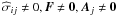 have not yet been discussed in the context of astrospheres. In principle, the stress tensor is needed to physically induce instabilities, which is typically simulated by “numerical” viscosity, because otherwise the required resolution is too high to be modeled.
3.5. Fluids including dust
Many bow shocks are observed in infrared radiation emitted by dust grains (Cox et al. 2012). van Marle et al. (2011) modeled the dynamics of the dust grains generated by the star. Far away from the star, neither the gravitational force nor the radiation pressure plays a role because both decay as r-2. Furthermore, these authors treated the dust as test particles: the dust particles experience a drag force by the plasma, but the plasma is not affected by the dust. This behavior is also found in the solar wind (Fahr et al. 1995).
Nevertheless, the dust dynamics are complicated and can be modeled using the Euler equation when external forces such as drag, Poynting-Robertson forces, and the Lorentz force are included.
In principle, dust grains can affect the plasma by sputtering of ions or atoms from their surface, which leads to mass, momentum, and energy loading of the plasma. To model this, additional balance equations are needed, as is a dust model, to describe their dynamics, which are important for the momentum and energy loading. With a gas-to-dust mass ratio of about 100 (Liseau et al. 2015), the plasma dynamics should not be affected by the dust, and we therefore did not take it into account here. From an observational point of view, especially using infrared observations from Herschel (Cox et al. 2012), the dust is important for detecting bow shocks.
4. Hydrodynamic shocks: single-fluid shocks
We here assume that the relative motion between the star and the ISM is supersonic (for subsonic relative speeds see Steinolfson 1994; Zank et al. 2013), and furthermore, that the shock structures are in quasi-stationary equilibrium, which means that they are at rest with respect to the star.
Now we concentrate on single-fluid hydrodynamic shocks, where we assume that the fluid is collisionless, consists of protons, and is polytropic with a coefficient γ = 5/3. Such a fluid behaves like a neutral perfect gas fluid, and all the gas dynamical methods can be applied (Ben-Dor 2007). For large-scale simulations of astrospheres see Arthur (2012), and for heliosphere simulations see Pauls et al. (1995), Fahr et al. (2000), and Izmodenov et al. (2003).
As pointed out by Baranov et al. (1971) and Pauls et al. (1995), the shock structure of the heliosphere consists of strong shock solutions, where the shocked Mach number M2< 1, and weak solutions, where the Mach number after the shock is higher than 1 (M2> 1), see also Izmodenov & Baranov (2006). Making the HD equation dimensionless by setting  (4)a factor f = vstTS/RTS in front of the ∇·() operator appears, which includes the characteristic scales for the speed, time, and length scales. The factor is one by construction when the speed is set equal to the constant supersonic stellar wind speed at the inner boundary v0 = vs, the timescale t0 to the scale the stellar wind needs to reach the TS T0 = tTS, and length scale to the stellar-centric distance to the TS R0 = RTS on the stagnation line. The dynamically independent values here are the stellar wind density and speed as well as the stagnation distances, which are determined by the total momentum conservation between the stellar wind and the ISM (see below). Thus, all different astrospheres can be modeled after solving for the dimensionless fluid and then scaling it back by using ρ0,vS, and RTS.
The initial mass density ρ0 and the terminal speed vs are prescribed at the inner boundary. The stellar-centric TS distance RTS is a function of the total momentum of the stellar wind and the ISM (see below).
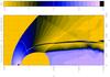 |
Fig. 2 Contour plot of the sonic Mach number M from an polytropic one-fluid simulation. The features described in the text and shown in Fig. 1 can easily be recognized. The kink at x = −250, and R = 1000 is caused by a reflection at the boundary of the integration region. Values are truncated at M = 2. |
Therefore, we no longer distinguish between different astrospheres (Arthur 2007, 2012), pulsar wind nebulae (Bucciantini 2002, 2014) or the heliosphere, as long as we can describe them by a single collisionless fluid without other interactions. In that sense, this section is generally applicable to all single-fluid astrospheres. Therefore, we use the dimensionless parameters below, and to save writings we drop the  in what follows.
4.1. Large-scale shock structure
The shock structure for a single collisionless fluid is sketched in Fig. 1, and a model is shown in Fig. 2. Most of the shock structures in a single-fluid description, such as the TS distance and the jump conditions, can be described analytically, or semi-analytically (for example, the AP and BS distance). Therefore, they can be used for a first estimate, and we discuss them in detail below.
In the hydrodynamic case each surface of flow lines can be replaced by a solid wall without changing the flow configuration. Thus we assume that the AP is represented by a solid wall that separates the two fluids, the stellar and the interstellar wind. Starting from the star, the stellar wind velocity jumps at the TS. Because it creates an oblique shock surface, a sonic line can be found at which the shocked Mach number M2 = 1. Between the stagnation line and the sonic line exists a strong solution (M2< 1), while beyond the sonic line the shock solution is weak M2> 1, that is, the transition from the supersonic stellar wind remains supersonic. In the tail direction a triple point T forms, where a slipstream or tangential discontinuity TD separates the supersonic from the subsonic flow. At this TD the pressure between the two flows is in equilibrium. Moreover, from the triple point T a reflected shock propagates toward the AP, where it is reflected again toward the TD, where it becomes reflected again. From the triple point a circular Mach disk extends toward the stagnation line.
The BS is detached from the blunt AP, where the distance  . Similar to the TS, the BS is an oblique shock surface, where a sonic line emanates.
To solve the Euler equations the inner boundary values are usually given by ρ0,v0 = vs,P0 (or the temperature T0 instead of P0). With the knowledge of RTS and the condition that the fluid inside the TS is polytropic and spherically expanding at constant speed, we have  Furthermore, the stellar wind at the inner integration boundary is always supersonic, that is, Ms,0> 1. The Mach number Ms increases as r2/3, meaning that it is by definition inversely proportional to the square root of the temperature. Thus, we expect huge Mach numbers at the TS, and following from this, that in this realm the flow is “hypersonic”, that is, M ≫ 1. In turn, the thermal pressure upstream of the TS is almost zero because it is lower than the ram pressure at the inner boundary and decreases with r− 10/3. The supersonic velocity v0 = vTS,1 remains constant until it reaches the TS.
4.2. Pressure and temperature in the hypersonic approximation
We can calculate the pressure downstream of the TS knowing RTS using the jump condition in the momentum equation. Assuming that the pressure inside the TS is negligible compared to the ram pressure, we obtain from the Rankine Hugoniot relation for the total momentum density  with
with  , and r0 is a reference radius (r0 = 1 AU for the heliosphere and r0 = 0.03 pc for λ Cephei). We easily derive the shocked pressure PTS,2 as
  (9)where ϑ is the shock angle, which is the angle between the upstream velocity and the shock.
At the nose ϑ = π/ 2 and all the values on the right-hand side are known by assumption. We can furthermore assume that the pressure in the region given by the intersection of the sonic line, the TS, the AP, and the stagnation line, is almost constant, because it is a subsonic flow. Thus we obtain a relation between the stellar-centric distances along the TS and the shock angle, which is not identical with a stellar-centric angle Φ to the same point on the TS.
Another nice feature of the hypersonic flow is that the temperature directly beyond the TS depends only on the initial velocity and the shock angle because the Mach number  increases inversely proportional to the temperature T1 = T0(r0/r)− 4/3. With this, we find
 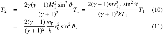 where m is the mass of a fluid particle and k is the Boltzmann constant. Here we additionally assumed that m = mp (proton mass mp).
This has the nice consequence that the temperature downstream of the TS determines the shock angle ϑ when v0 is known. Furthermore, v0 can be determined measuring TTS, where ϑ = π/ 2. For λ Cephei the temperature at the TS for ϑ = π/ 2 and v0 = 2500 km s-1 is T2,TS = 1.2 × 10⁸ K. From an observational point of view, the BS is easier to observe, and for v0 = 80 km s-1 the temperature is T2,BS = 1.4 × 10⁵ K.
Typically, v0 is known as the terminal velocity from stellar wind models, therefore by measuring the temperature at the TS in the nose direction (i.e., at the stagnation line), we can determine if the polytropic coefficient γ = 5/3. This amounts to a test whether the assumption of a mono-atomic gas holds. In addition, the same is true for the BS when the interstellar Mach number is high enough.
This holds true for most of the models where no other interaction with the hypersonic stellar wind appears, like charge exchange with neutrals. This includes cooling or heating inside the TS because there the temperatures and densities are low, so that neither cooling nor heating is effective (see below). This should also apply to MHD models in which the magnetic field pressure inside the TS is negligible compared to the ram pressure. Models including mass, momentum, and energy loading have to be excluded because the stellar wind speed is affected in those.
4.3. Termination shock distance
Next we determine the TS distance. First we recognize that since there is no mass flow through the AP, vn,I,2 = vn,S,2 = 0, where IandS denote the interstellar and stellar conditions, and n describes the velocity component normal to the shock.
Inserting this into the momentum conservation, we derive at the AP PI,2(AP) = PS,2(AP). Because the total momentum is conserved along a flow line, which here is the stagnation line, the pressure at the AP is the same as that directly after the BS: 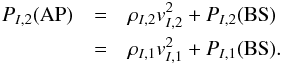 (12)Inside the AP a similar condition holds for the stellar wind (replacing the index I by S and BS by TS). Thus we derive at the AP
 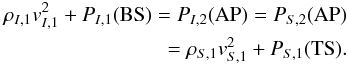 (13)We can express the density of the stellar wind by its mass-loss rate
  and its terminal velocity | | v∞ | | = | | v0 | | (= vS,1 = const. in the supersonic stellar wind region) by
  (14)or
 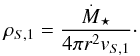 (15)Taking Eq. (13), rearranging it, and inserting Eq. (15), leads to
 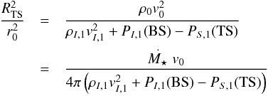 (16)with
  .
.
The thermal pressures in the supersonic media can usually be neglected compared to the ram pressure, at least for high Mach number flows. Then Eq. (16) reduces to 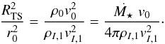 (17)RTS is the TS distance at the stagnation line. We wish to emphasize that the TS distance is the only distance that can be determined without any other assumption in addition to the momentum conservation and the polytropic behavior of the stellar wind. The TS distance is not the stagnation distance. The latter is defined as the distance at the stagnation line where the (shocked) interstellar flow speed and the shocked stellar wind speed are both zero, which is the AP distance RAP.
The r-dependence of the density and velocity is unknown in the shocked stellar wind region, that is, in the inner astrosheath. Similarly unknown is the functional dependence of those in the shocked interstellar wind region, that is, in the outer astrosheath. Therefore the stagnation distance or AP standoff distance cannot be determined without further assumptions.
4.3.1. Astropause distance I: in upwind direction
The AP or stagnation distance is often described using a flow potential (Parker 1961; Suess & Nerney 1990) or using the thin-shell approximation (Baranov et al. 1971; Dyson 1975; Raga et al. 2014), where a dependence of r from the stellar-centric angle Φ to a point on the AP or BS is formulated. As was discussed in Zank (1999), these are a rather poor approximations.
The reason is that the shock normal is in general not parallel to the radius vector (see Fig. 3). The shock angles ϑsl,i and the flow deflection angle ϕsl,i at the sonic points, which are the points at the intersection of the sonic line with TS (index S) and with the BS (index I), see Fig. 1, can be calculated setting M2 = 1 to determine the flow deflection angle. For the interstellar flow this is not a problem because there we know the Mach number MI,1 in front of the BS and for the stellar wind flow we assume MS,1 ≫ 1. The green line shows that the flow deflection angle ϕ changes dramatically when the shock angle ϑ varies only very slightly. For a wide range of shock angles the flow pattern can therefore be different, but for Mach numbers MI> 2, the flow deflection angles ϕ and the shock angle ϑ are approximately constant. The overall shock structure depends on both the stellar and interstellar ram pressure, but the two angles ϕ and ϑ do not, which means that it cannot be expected that purely geometrical considerations lead to reliable results.
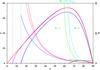 |
Fig. 3 Dependence of the flow deflection angle with respect to the shock angle for different Mach numbers M1 (solid lines). The black, blue, magenta, and red lines correspond to M1 = 1.1,4,10,and100, respectively. To the right of the dotted vertical lines a physical solution exists for the corresponding Mach number, while to the left it does not. The dashed lines show the dependence of the shocked Mach number M2 from the shock angle ϑ (scale on the right vertical axis). If M1 varies, this does not lead to strong variations of ϑ around the sonic points, where M2 = 1 and ϑ ≈ 57 − 64 deg for all Mach numbers M1. But the variation of the flow deflection angle ϕ (left vertical axis) is large, as shown by the green dashed line. This line also separates the region between the weak solution (M2> 1, left from the green dashed line) and the strong solutions (M2< 1 right of the green dashed line). At this green dashed line M2 = 1 is close to the cyan dashed line, where the shock angle (ϑ) reaches a maximum. |
The deviation of the shocked interstellar flow in particular violates the assumption of a parallel subsonic flow at infinity and the irrational condition that is needed to derive the stagnation distance from the flow potential. The thin-shell approximation is usually violated because the distance between the TS and AP, and to a lesser extent between the AP and BS, are not shorter than the TS distance. As we discuss below, the distance between the AP and the BS shrinks remarkably as a result of cooling effects. But then the structure of the astrosphere is more complicated.
 |
Fig. 4 Distance between BS and AP as a function of the compression ratio s. The red line shows the Δ(s) with a = 1, the blue dashed line the same for a = 0.5, and the black dashed line for a = 1. |
There is no simple functional dependence between the stellar-centric angle Φ and the ISM shock angle ϑism or the ISM flow deflection angle ϕism. The latter depends on the Mach number Mism of the inflowing ISM and also on the shape of the BS. The latter shape is also influenced by the AP, which in turn is formed by the shape of the TS. The curvature of the latter is also shaped by the ram pressure of the ISM (Mach number Mism), which is shown by the following consideration: with a varying ram pressure of the ISM, the distance of the TS changes. If we assume that the region between the TS at the stagnation line and sonic point on the TS can be described by a sphere with radius RTS, then it is obvious that the curvature of the TS around RTS changes as  . Then for low decreasing interstellar ram pressures (Mach number Mism> 1) the flow deflection angle ϕsl,ism at the sonic point decreases and the upwind distance Δ between AP and BS increases, while for high increasing interstellar Mach numbers Mism ≫ 1 the distance Δ decreases, but the sonic shock angle ϑsl,ism and the sonic flow deflection angle ϕsl,ism remain approximately constant. Thus the stellar-centric position angle Φ must depend on ϑism and ϕism. The sonic points on the TS are given by the stellar Mach number Ms, which is always huge, and thus we can conclude that the sonic shock angle ϑsl,s and the sonic flow deflection angle ϕsl,s are not affected by the change of Mism, only the curvature of the TS is changed and moves the sonic lines toward or away from the inflow axis.
The shape of the AP cannot be determined easily because this is a pressure equilibrium surface, specifically, a tangential discontinuity. Across this structure only the thermal pressure has to be balanced on both sides, while the tangential velocity, the temperature, and the density may jump. The normal velocity component is zero because no mass is transported through a tangential discontinuity. We just state here that a contact discontinuity is a different feature, which appears in an MHD shock structure, where the normal magnetic field does not vanish. Then the density can jump, while all other quantities (tangential velocity and magnetic field, the sum of thermal and magnetic field pressure) are continuous across a contact discontinuity. Nevertheless, the determination of the AP shape can be formulated as an inversion problem, knowing the (parabolic) shape of the BS, the shape of the AP, especially the distance between AP and BS, can be estimated (Schneider 1968; Schulreich & Breitschwerdt 2011).
The stellar-centric AP distance can also be calculated using the approach to determine the distance between the AP and the BS, as we discuss below.
4.3.2. Bow shock distance to the astropause
We assume that the AP is locally approximated by a solid sphere with radius RAP. For this blunt body an approximate BS distance using the two-dimensional continuity and energy equation can be determined (Olivier 2000) for γ = 5/3: 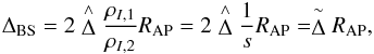 (18)where ΔBS is the distance between the stellar-centric BS and the AP (ΔBS = RBS − RAP), s is the compression ratio s = ρI,2/ρI,1 and
  is given by
 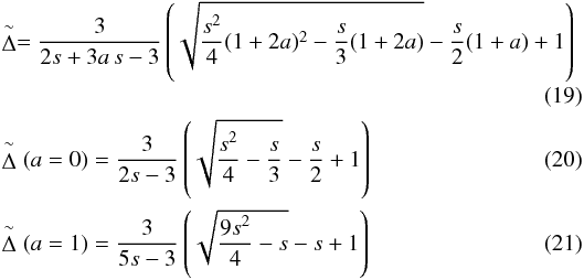 where a is the derivative of the normalized tangential velocity at RAP, that is, a = ∂u/∂ϕ. Assuming that the tangential velocity vanishes at the BS in the inflow direction, we obtain
  for the above compression ratio s = 3.87 for the ISM around λ Cephei.
Earlier approaches (e.g., Barnette 1993) found numerically  (22)For non-reactive gases Van Dyke (1958) determined ΔBS also numerically by
 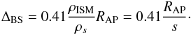 (23)The flow pattern around a sphere with diameter RTS was calculated and experimentally verified by the above authors. If we assume that around the nose the AP can be described by a sphere with the radius RAP, the stellar-centric distance of the AP, we can use the above estimates to determine Δ. The BS distance from the center is
  (24)Farris & Russell (1994) approximated the blunt body by a conic section, and with a given radius of curvature, these authors found the bow shock distance as
  (25)which can also be applied to low Mach numbers, for which the BS then moves to infinity. RC is the radius of curvature defined as 1 /κ, where κ is the curvature. For a sphere with radius RAP, we have RC = RAP. The latter equality in Eq. (25) follows from the Rankine-Hugoniot equations for the compression ratio.
For hypersonic flows Eq. (25) can be simplified to  (26)Equations (19) and (25) give almost identical results for the respective parameters, and the hypersonic limit Eq. (26) is also acceptable, especially for λ Cephei, as can be seen in Table (5). The problem of determining RAP remains, however.
4.3.3. Astropause distance II
We use the same approach as above to determine the AP distance from that of the TS. Assuming now that the supersonic wind approaches a hollow sphere, we obtain with the compression ratio ss ≈ 4 of the stellar wind  . This approach also nicely reproduces the AP distances RAP = (1 + Δ)RTS, as given in Table 5.
4.3.4. Tail termination shock distance
In the tail direction, the flow along the AP and the tangential discontinuity are almost parallel. The only pressure that has to be balanced, therefore, is the thermal pressure of the ISM, which then also has to be balanced in the subsonic tail region. By replacing the ram pressure in Eq. (16) by the thermal pressure, the tail distance of the TS can be determined as  (27)This is not a good approximation, see Table 3, because instead of the shocked, the interstellar thermal pressure should be used, which can be higher than the undisturbed pressure. Nevertheless, the undisturbed pressure alone can be determined analytically.
4.3.5. Temperature and pressure
For high Mach number flows, we can replace the Mach number using  , from which follows
 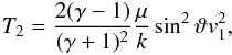 (28)with the average mass μ = ∑ sasms and the Boltzmann constant k. as and ms give the abundance and mass of a particle of species s ∈ { p,He+,He++,... }. We also dropped the indices SandI because Eq. (10) holds in general.
Hence, the shocked temperatures upwind and downwind of the TS are identical, and they vary like sin2ϑ along the TS. This means that in the region between the nose (ϑ = 90°,sin2ϑ = 1) and the sonic point at the BS (ϑ ≈ 63° andsin2ϑ ≈ 0.7), the temperature directly beyond the TS changes by 30%. The density jump for hypersonic flows is roughly 4, and consequently, the thermal pressure varies by 30% along the TS in the subsonic region.
Moreover, if we know the temperature along the shock, the shock angle ϑ can be determined for hypersonic flows, which then determines the flow pattern directly behind the shock. This is also valid for interstellar flows with sufficiently high Mach numbers, especially around the nose region of the BS, where ϑ> 60°. This means that the temperature in the nose direction can be used to determine the interstellar flow speed using Eq. (10).
Between the sonic lines the flow is subsonic, therefore the thermal pressure is nearly constant. This is also true beyond the Mach disk (see Sect. 4.3.6), and the pressure can therefore be estimated by calculating the pressure at the nose for the interstellar and stellar fluid, and the thermal pressure at the tail for the stellar flow. For the hypersonic case we find from the Rankine-Hugoniot relation 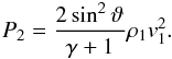 (29)Applying these approximations to the stellar wind, which is highly supersonic (for the λ Cephei stellar wind, Mach numbers at the TS are M1,S ≈ 7000), the stellar wind thermal pressure is negligible compared to the stellar wind ram pressure and thus does not influence the dynamics of the flow inside the TS. This is convenient, because only the stellar wind density and velocity can be determined from observations and the theory of stellar atmospheres. But that is all what is needed to describe the dynamics of the flow inside the TS in the single-fluid model.
4.3.6. Mach disk
The numerical experiments show that the Mach disk can be fitted by a circle, the center of which is shifted from the star toward the tail. The translation parameter and the radius of the circle have not been determined analytically up to now.
5. Hydrodynamic shocks: including cooling and heating functions
The great extent of astrospheric shocks around hot stars can cause an efficient cooling of the flow inside the BS. Many different cooling functions are discussed in the literature (see Rosner et al. 1978; Dalgarno & McCray 1972; Sutherland & Dopita 1993; Schure et al. 2009; Mellema & Lundqvist 2002; Townsend 2009; Reitberger et al. 2014a), which reflects the different compositions and states of the ISM. The piecewise analytic representation by Siewert et al. (2004) lies in between these extremes, and we have chosen this representation for our model of λ Cephei. The cooling functions can differ by orders of magnitude, especially at lower temperatures (Dalgarno & McCray 1972), depending on the metallic abundances. These lower temperatures are usually reached when a low Mach number BS appears, which is typically the case for low, but still supersonic interstellar wind velocities. In the tail regions such lower temperatures can also be reached. The shocked stellar wind is usually above 108 K, except for the flanks of the astrosphere, where oblique shock transitions with weak solutions appear (M2> 1).
The thermal pressure is higher than the ram pressure in subsonic regions. By neglecting the ram pressure in the energy equation and assuming a polytropic behavior of the gas, we can therefore write the energy equation approximately as (also discussed in Scherer et al. 2014) 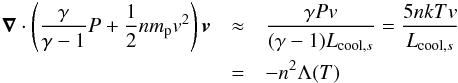 (30)replacing ∇ by the inverse subsonic cooling length, Lcool,s can be estimated as
 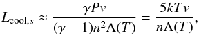 (31)and the subsonic cooling time τcool,s
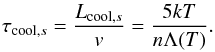 (32)This cooling time is by up to a factor 3 the same as that given in Sutherland & Dopita (1993). Vice versa, in a hypersonic wind we neglect the thermal pressure and obtain analogously
 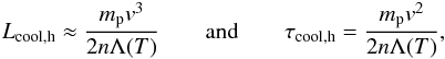 (33)where Lcool,h and τcool,h are the hypersonic cooling length and time.
The heating function by photoionization and some supplemental heat source is discussed in Kosiński & Hanasz (2006), but see also Reynolds et al. (1999): 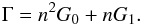 (34)With the constants G0 = 10-24 erg cm3 s-1 and G1 = 10-25 erg s-1 and replacing the right side of Eq. (30) by Γ, we obtain
 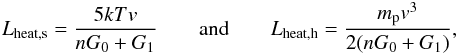 (35)and the heating times τheat,s,τheat,h by dividing the respective heating lengths by the speed v.
The cooling and heating lengths can be interpreted as the distances at which the flow is significantly cooled or heated. Moreover, it gives an r-dependence of the flow in the outer astrosheath, which allows determining the distance between the BS and the AP, which is in the order of a cooling length (depending on the shocked temperature).
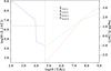 |
Fig. 5 Cooling lengths. The number density and speed are fixed at n = 10 cm-3 and v = 80 km s-1. All scales are logarithmic. On the x-axis we display the temperature, while the characteristic length is shown in AU on the left y-axis and in parsec on the right y-axis. The dashed vertical line denotes the temperature where the ram pressure equals the thermal pressure. |
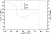 |
Fig. 6 Cooling lengths. The number density and speed are fixed at n = 10 cm-3 and v = 2500 km s-1. For the meaning of the subscripts see text. |
Even without running numerical models, we can elicit some information about the thickness of the outer astrosheath, especially about the distance between the BS and the AP (see Scherer et al. 2014). For convenience these estimates are repeated here.
The hot shocked ISM is mainly affected because the number densities in the shocked ISM are higher by a factor of 3.6, which is the compression ratio between the shocked and unshocked ISM, and according to Eq. (10), the shocked temperature T2,I ≈ 8 × 10⁴ K. In the range where T ≈ 103–105 K, most of the discussed cooling functions are similar, which means that they jump three orders of magnitude around 104 K. Above that temperature, the different cooling functions lead to a more or less efficient cooling until the temperature falls below ≈ 104 K. Thus, the time in which the bow shock reaches its final position can differ because of the cooling efficiency in the outer astrosheath. Moreover, because the astropause is a pressure equilibrium surface that balances the shocked stellar wind and ISM thermal pressure, it follows from the ideal gas law P = 2nkT that the number density n in the outer astrosheath toward the AP must increase to balance the stellar wind thermal pressure. This is different from a purely hydrodynamic model, where the density and pressure are almost constant in both astrosheaths. (The densities differ on both sides of the AP, but the pressures are balanced.)
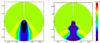 |
Fig. 7 Number density for the pH-model (left panel) and the CH-model (right panel). Both models are still not in quasi-stationary equilibrium, the physical time is ca. 160 kyr. The length scale is in AU, which corresponds to a box size of 24 pc. |
In the inner astrosheath, the region between the AP and the TS, the number density is on the order of n = 10-3 cm-3 and the velocities are on the order of v = 600 km s-1, and thus cooling and heating length scales, depending on v and n, become huge: the cooling is no longer important in the inner astrosheath and inside the TS. The heating length scale depends only on the number density n and also increases to scales much larger than the distances inside the AP. This holds true at the inner integration boundary, but inside of this, cooling and heating can become more important because the number density increases with decreasing stellar-centric distance. For stellar wind velocities of v = 2500 km s-1, it can easily be estimated that the temperature must be higher than T ≈ 107 K (see Fig. 6). Figure 5 shows that in the hypersonic region cooling dominates for temperatures of ≈ 104 − 3 × 10⁷ K, while for temperatures lower than 104 K heating is the dominant process. Nevertheless, these length scales are so large (in the order of 104 pc) that they exceed the TS distance by far, especially in the tail. Thus they may be neglected to first order. If the thermal pressure starts to dominate (beyond T ≈ 3 × 10⁷ K), heating is by far the dominant process, with characteristic scales of around 1 pc and linearly (Eq. (33)) increasing with temperature.
Because of the huge ram pressure of the stellar wind, we can from a dynamical point of view safely neglect heating and cooling inside the TS, however, as it does not influence the polytropic expansion of the stellar wind. Therefore, we can neglect the thermal pressure compared with the ram pressure at the TS.
From the discussion above, we conclude that heating and cooling are dynamically important only in the shocked and unshocked ISM, while for the stellar wind it can be neglected, except in the extended tail regions.
5.1. Temperature and pressure
The same considerations hold for the shocked temperature and pressure, as discussed in Sect. 4.3.5. We only have to assume that the shocks are not radiative, meaning that the  as discussed in Sect. 3.1, which means that the thickness of the shocks is so small that no collisions occur and the excitation of atoms is negligible as well. This is the case for astrospheres with stationary shocks because the material has enough time and space to flow around the obstacles. For colliding shocks or shocks in binary systems, this is not true (Reitberger et al. 2014b; Parkin et al. 2011).
For the single-fluid case with cooling or heating, the supersonic ISM flow hits the BS in the same way as without cooling. Thus the temperature jump at the BS is given by the ISM speed (Eq. (10)) and also the shock angle ϑ, while for the pressure (Eq. (29)) the ISM density is additionally needed.
To summarize, measuring the temperature along the shock as well gives the interstellar wind speed when cooling and heating are active.
6. Numerical models
In Fig. 7 we show the number density in the “ecliptic” for both the pH- and CH-model. A stationary equilibrium for the pH-model is reached after roughly 1.5 Myr, while it takes about 2.5 Myr for the CH-model to reach stationary state. We compare the two models after 1.5 Myr to emphasize the differences in time evolution.
In Fig. 8 some important quantities along a radius vector in the ecliptic plane (ϑ = 0°) are shown. The pH and CH-model are asymmetric, therefore lines in the figure are sufficient to show the essential variations. While in the pH model the density at the TS jumps by a factor four (strong shocks), it remains constant up to the AP. There it increases by orders of magnitudes to the shocked interstellar value, and finally decreases by a factor ≈ 3.8 at the BS to the interstellar value. The ISM number density at the AP is slightly higher at the AP because here the velocity tends to zero and the gas is piled up.
For the CH-model the behavior between the TS and the AP is analogous. The ISM gas density is lower than in the pH model because the cooling also takes place in the ISM, and a new equilibrium state of the ISM is attained just inside the outer boundary conditions.
The CH-model again shows a pile-up of the ISM gas at the AP, while it almost decreases to the new ISM value shortly after the AP. Then the ISM number density increases further by a factor 50. This compression is about 12 times stronger than the compression for a pure gas dynamic shock, where we have defined the compression ratio s as the ratio of the number density in front of the shock and behind it. In the CH-model the increase of the density to its highest value is reached after 0.05 pc, and therefore we took the value at this position to calculate the compression ratio. This behavior is also described in Mackey et al. (2015), and it leads to a division of the outer astrosheath into a cool and hot part (see below).
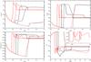 |
Fig. 8 Number density, temperature, thermal pressure, and the Mach number. The black lines describe them for the model without and the red lines the parameters for the model with cooling and heating. The solid lines show the parameters along the stagnation line (i.e. 0°), while the dashed lines are those along the pole (90°), and the dotted lines along the tail direction (180°). The upper left panel shows that the number density for the model without cooling and heating jumps at the TS and BS by a factor of four, while for the CH-model the density at the TS also increases by a factor of four, but at the BS it increases by more than a factor of 10. In both cases the temperature jumps by orders of magnitudes at the shocks (upper right panel). The lower left panel shows the thermal pressure, which is discontinuous at the shocks, but in both cases more or less continuous at the AP along the stagnation line. The lower right panel shows the Mach number. The inlet is a linear plot in the Mach number between 0 and 3. It shows only the Mach numbers in the CH-model to present its structure. The CH-model is presented after 150 kyr, while the pH model is fully developed (kyr). |
The distance between the first peak as seen from the BS to the AP is ≈ 0.05 pc in the CH-model, which is roughly the cooling length. The distance between the AP and the BS is roughly 0.2 pc in the CH-model and 0.4 pc in the pH model. The distance between the TS and the AP in both models is approximately 0.2 pc. Together, the distance between the TS and BS is approximately 40% that of the stellar-centric distance to the TS. This again shows that the thin-shell approximation is not valid because the outer shell (between TS and BS) has almost the same size as the inner shell (between origin and TS). In addition, the density increases by a factor of more than four at the flanks at 90° and in the tail direction 180°, and the thickness of the outer astrosheath is almost the same in both models.
As shown in the lower left panel Fig. 8, the thermal pressure is almost the same in the inner and outer astrosheath and is continuous at the AP, as required for a tangential discontinuity. This holds also true for the other two directions.
The temperature is displayed in the upper right panel of Fig. 8. It increases by orders of magnitudes at the TS in both models and remains constant in the pH model until it reaches the AP, where it decreases by orders of magnitudes to the shocked ISM value, and finally decreases at the BS to unshocked values. The sudden increases at the AP are slightly smeared out for the TS at the polar direction, while the BS does not exist in the tail direction. The increase of the temperatures at the TS in the CH-model is almost the same as for the pH model, but then it decreases strongly at the AP to the unshocked ISM value, shows a peak in the direction of the BS, and finally returns to the unshocked value. In the polar direction, the increase toward the AP in the inner astrosheath is similar to that for the pH model, but after the AP it directly drops to the unshocked value in the ISM. There is no longer a BS at this position. In the tail direction, the temperature remains at the high value after the shock for both models.
The Mach numbers are shown in the lower right panel of Fig. 8. Those of the CH-model in the nose direction and 90° are separately displayed in the inset. Here the scale on the vertical axis is linear to show the complexity. The Mach number along the stagnation line drops after the TS to values below one and decreases further to the astropause. There it quickly increases and shows some structure in the outer astrosheath, namely a hot outer astrosheath (HOA) and a cool outer astrosphere (COA). These structures differ in the HOA and COA. Moreover, it depends on the choice of the CHF. Thus a detailed comparison between the CHF is required, which may also be reflected in the observations, leading to some information about the composition of the ISM because the CHF depends on it (e.g., Sutherland & Dopita 1993).
From this discussion we can extract much information about the shock structure: in Table 2 we list the inner boundary values for the stellar wind of λ Cephei at 0.03 pc with those at the outer boundary at 12 pc for the ISM. The polytropic index is fixed in the entire integration region to γ = 5/3. Using this set of parameters, we can determine the sound speeds, Mach numbers, and pressures as well as the distances to the TS in nose and tail direction. The latter two are compared with the modeled distances. The results are shown in Table 5 together with the compression ratios (s = ρ2/ρ1). Finally, we estimated the values of the stellar wind at the TS, using the r dependence for polytropic expanding stellar wind (i.e., ρ ∝ r-2, T ∝ r−4/3, P ∝ r− 10/3, and M ∝ r2/3), which are displayed in Table 5, and those for the interstellar parameters at the BS, shown in Table 4. Finally we display in Table 6 the shock angles and flow deflection angles at the intersection of the sonic lines with the TS and BS.
Initial values for the stellar wind (SW) at the inner boundary 0.05 pc and the interstellar medium (ISM) at “∞”.
In Tables 4 and 6 we show the results from the pH and CH-models. They agree well with the analytic results. The tables also show that the values at the TS and BS do not change much from one model to the next. In the outer astrosheath, the flow behaves differently in both models. This means that the analytic values shown in Tables 2 to 6 can be used as a first estimate for an astrosphere.
Characteristic distances.
Parameters of the ISM in front of the shock (upstream x = 1) and behind it (downstream x = 2).
Stellar wind parameters in front of the shock (index 1) and behind it (index 2).
 |
Fig. 9 Left panels: the shock distance depending on the stellar-centric angle Φ counted from the inflow direction. Cyan shows the distance of the BS, orange that of the TS. Blue shows the variation of the temperature along the BS and red that of the TS. Right panels: the shock angles at the BS (blue) and the TS (red). The upper two panels display the quantities for the pH-model, the lower panels those for the CH-model. For more details see text. |
The CHF appears only in the energy equation, not in the momentum equation. The latter is weakly influenced through thermal pressure changes induced by the energy equation. The reason for the lack of momentum changes is that the energy loss is a scalar that is radiated in all directions, without changing its sign. The momentum is a vector quantity that in the rest frame of a particle also radiates in all directions, whith two movements cancelling each other. This means for a photon emitted in one direction that there will be on average one photon with the same moment emitted in the opposite direction. Thus the momentum loss can be neglected.
The cooling and heating also introduce a notorious instability, as already discussed in Schwarz et al. (1972) and Scherer et al. (2015b). This instability results in wiggles along the BS. By comparison with observations, the wavelength of these wiggles may be used to determine the CHFs in mind, if it can be assumed that the wiggles depend in a characteristic way on the magnitude of the CHF.
Finally, we applied the hypersonic formula for the dependence between the temperature and the inflow speed and shock angle, Eq. (10), to estimate the shock angle. In Fig. 9 we display the shock distances for both the TS and the BS along the stellar-centric angle Φ counted from the inflow direction. The left panels of Fig. 9 show the shock distances and the temperatures along them, but in the shocked region, the TS and BS. The shocked temperatures after the TS in the inflow and in the tail direction are almost equal, in agreement with the Rankine-Hugoniot relations. In the right panels the shock angles along both shocks for both models are shown. In the upper left panel of Fig. 9 the shocked temperature (blue line) upstream of the BS at roughly 15° and 345° has a depression that strongly decreases to values of around 30°. When the shock angle reaches 60°, the decrease becomes even larger and the hypersonic approximation is no longer valid. This occurs at the sonic points, beyond which a weak shock solution applies.
The figure also shows a similar feature at the TS shortly after 40° (320°), where the shocked Mach number also becomes 1 and the shock angle ≈ 63°. In the tail direction, at about 150° (210°), another depression is visible, after which we find a strong increase of the shock angle to almost 90°. These depletions occur at the triple point and they increase at the Mach disk to the required 90° shock angle at the downwind axis.
First the astrosheath is divided into a cool and hot part (see also Mackey et al. 2015). The shocked Mach number is everywhere greater than one in both outer astrosheaths. This is in contrast to the pH model, where the Mach number is lower than one in the nose direction. Thus the sonic line between the BS and AP disappears, and the outer astrosheath is supersonic everywhere. In the inner astrosheath, the sonic line starts at the same point as in the pH case, but then bends in the middle of the inner astrosheath into the tail direction, where it then ends in the AP. The triple point is still existent, but the bending of the shock is much smoother. The reflected shocks vanish. Because the triple point still exists, the Mach disk remains.
While in the HOA the number density jump after the shock is similar to that in the pH case, it decreases toward the COA, to increase to much higher values in the COA than for the pH model. In front of the AP a proton wall is created in this way because the normal velocity decreases to zero at the AP (no mass transport through it).
Similarly for the temperature: it increases after the shock passage in the HOA and then quickly becomes lower when the cooling starts to operate. It almost reaches the same values as those in the ISM. The pressure in the HOA and COA remains more or less constant, as can be inferred from the ideal gas equation P = 2nkT. Accordingly, when the density increases, the temperature has to decrase to keep the pressure constant. This behavior is shown in Fig. 8.
For the CH-model the shock angle of the TS behaves similarly, but that of the BS is more or less arbitrary. The reason for the latter is that the HOA is very thin around the inflow direction, and determining the temperature is difficult. The flow becomes even hotter in the flanks of the astrosphere, which is caused by the interaction of flow from the nose direction and the directly shocked stellar wind in the outer astrosheath regions.
The curves shown in Fig. 9 are ragged because of the low resolution in the Φ direction and the strong dependence on arcsin.
Derived shock parameters: the shock angle ϑsl,i and flow deflection angle ϕsl,i at the intersection of the sonic line and the TS (i = sw) and that at the BS (i = ism) are displayed together with the compression ratios sj at the TS in nose direction (j = n), the tail direction j = t and at the BS j = ism.
7. Large-scale shock structure including cooling and heating
We combine all our findings in the sketch shown in Fig. 10.
The structure of astrospheres including heating and cooling differs from those without it because the structure of the former strongly depends on the magnitude of these effects. They may not play a role at all, as is shown by the example of the heliosphere, where the cooling and heating lengths are much longer than the dimension of the heliosphere. However, for massive stars with huge astrospheres, the characteristic cooling and heating lengths are shorter than the characteristic scales, like the distances between the BS and AP.
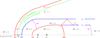 |
Fig. 10 Sketch of an astrosphere with strong cooling and heating effects. The sonic lines are different from those in Fig. 1, and in some region the Mach number has changed. The boundary between the hot and cool outer astrosheath is marked with a dashed green line. The changes in the Mach number are indicated in red. |
8. Conclusions
Astrospheres with cooling and heating in general have a different structure from those without it. In contrast to Mackey et al. (2015), we used the Mach number as the dynamically most important parameter to describe the structure of such an astrosphere. We found that the outer astrosheath is separated into a cool and a hot part, but there is more fine structure when using the Mach number as structuring parameter. The latter is interesting for acceleration processes of energetic particles (Scherer et al. 2015b).
Derived parameters for the stellar wind (SW) at the inner (at 0.05 pc) and for the interstellar medium (ISM) at the outer boundaries (at “∞”).
We gave an in-depth analysis of a pure hydrodynamical single-fluid (pH-) model and compared it with a model that also included heating and cooling effects (CH-model). We compared some characteristic parameters of the two models with those obtained by the Rankine-Hugoniot relations for a single-species fluid. We found good agreement with the pH-model, while for the CH-model only the relations along the TS give reliable results.
We also showed that the thin-shell approximation is not valid in this context because the inner and outer astrosheath are comparable everywhere with the region inside the TS. Moreover, from theoretical considerations we are led to the same result because the shock angle is not 90° and no statement about the flow deflection angle can be given in general.
We discussed the application of the Rankine-Hugoniot relations to the models with and without cooling and heating. With these relations the conditions at the TS and BS can be estimated. We also showed that in the pH model only the TS distance can be estimated with good accuracy, while the AP and BS distances are difficult to determine because they do not have an explicit r-dependence. For the CH-model, we can estimate at least the thickness of the astrosheath using the cooling lengths defined above.
We also showed that for hypersonic ISM flows the temperature along the BS depends only on the unshocked ISM speed and the shock angle ϑ. Thus, measuring a temperature variation along the BS can give the unshocked ISM speed at the stagnation line and the shock angles along the BS. Because of the high Mach number (hypersonic) stellar wind flow, the thermal pressure (or equivalently temperature) does not play a dynamical role until the flow reaches the TS. Directly after this, the thermal pressure (or temperature) is determined by the flow speed and the shock angles along the TS. For modeling purposes the knowledge of the stellar wind speed and densities at a given position are therefore sufficient to model the astrosphere. Nevertheless, an approximate value has to be allocated in most of numerical codes, which should be low enough. We also showed that the compression ratio at the BS in the CH-model is much higher than in the pH-model. The velocity divergence at the TS is similar, but is much more compressed in the CH-model.
We also demonstrated that the cooling or heating is mainly effective in the outer astrosheath because there the densities are high and speeds low enough to enable an efficient cooling, while in the inner astrosheath the densities are very low and the bulk speed is very high, so that the cooling length scales are much longer than the TS distance, and thus the cooling and heating do not operate efficiently.
Acknowledgments
K.S., H.F., J.K., and T.W. are grateful to the Deutsche Forschungsgemeinschaft, DFG, funding the projects FI706/15-1 and SCHE334/10-1. D.B. and K.W. were supported by the DFG Research Unit FOR 1254. K.S. and H.F. appreciate discussions at the team meeting “Heliosheath Processes and Structure of the Heliopause: Modeling Energetic Particles, Cosmic Rays, and Magnetic Fields” supported by the International Space Science Institute in Bern, Switzerland.
References
- Alexashov, D. B., Chalov, S. V., Myasnikov, A. V., Izmodenov, V. V., & Kallenbach, R. 2004, A&A, 420, 729 [NASA ADS] [CrossRef] [EDP Sciences] [Google Scholar]
- Alouani-Bibi, F., Opher, M., Alexashov, D., Izmodenov, V., & Toth, G. 2011, ApJ, 734, 45 [NASA ADS] [CrossRef] [Google Scholar]
- Arthur, S. 2007, Rev. Mex. Astron. Astrophys., 30, 64 [NASA ADS] [Google Scholar]
- Arthur, S. J. 2012, MNRAS, 421, 1283 [NASA ADS] [CrossRef] [Google Scholar]
- Baranov, V. B., Krasnobaev, K. V., & Kulikovskii, A. G. 1971, Sov. Phys. Doklady, 15, 791 [Google Scholar]
- Barnette, D. 1993, Program SHOCKS: Quickly Estimating Super- and Hypersonic Inviscid Flow Parameters., Tech. Rep., Sandia National Laboratories, Albuquerque, New Mexico [Google Scholar]
- Ben-Dor, G. 2007, Shock Wave Reflection Phenomena (Springer Science+Business Media) [Google Scholar]
- Blasi, P. 2013, Astron. Astrophy. Rev., 21, 1 [Google Scholar]
- Bouquet, S., Romain, T., & Chieze, J. P. 2000, ApJS, 127, 245 [NASA ADS] [CrossRef] [Google Scholar]
- Bucciantini, N. 2002, A&A, 387, 1066 [NASA ADS] [CrossRef] [EDP Sciences] [Google Scholar]
- Bucciantini, N. 2014, Astron. Nachri, 335, 234 [NASA ADS] [CrossRef] [Google Scholar]
- Bzowski, M., Swaczyna, P., Kubiak, M. A., et al. 2015, ApJS, 220, 28 [NASA ADS] [CrossRef] [Google Scholar]
- Chashei, I. V., & Fahr, H. J. 2013, Ann. Geophys., 31, 1205 [NASA ADS] [CrossRef] [Google Scholar]
- Chashei, I. V., & Fahr, H. J. 2014, Sol. Phys., 289, 1359 [NASA ADS] [CrossRef] [Google Scholar]
- Courant, R., & Friedrichs, K. O. 1948, Supersonic flow and shock waves (New York: Interscience) [Google Scholar]
- Cox, N. L. J., Kerschbaum, F., van Marle, A. J., et al. 2012, A&A, 543, C1 [NASA ADS] [CrossRef] [EDP Sciences] [Google Scholar]
- Dalgarno, A., & McCray, R. A. 1972, ARA&A, 10, 375 [NASA ADS] [CrossRef] [Google Scholar]
- Decin, L., Cox, N. L. J., Royer, P., et al. 2012, A&A, 548, A113 [NASA ADS] [CrossRef] [EDP Sciences] [Google Scholar]
- Downes, T. P., & Drury, L. O. 2014, MNRAS, 444, 365 [NASA ADS] [CrossRef] [Google Scholar]
- Dyson, J. E. 1975, Ap&SS, 35, 299 [NASA ADS] [CrossRef] [Google Scholar]
- Edney, B. E. 1968, AIAA J., 6, 15 [NASA ADS] [CrossRef] [Google Scholar]
- Emanuel, G. 2000, in Handbook of Shock Waves, eds. T. E. Gabi Ben-Dor, Ozer Igra (Academic Press), 1, 186 [Google Scholar]
- Fahr, H. J. 1990, A&A, 236, 86 [NASA ADS] [Google Scholar]
- Fahr, H. J., Scherer, K., & Banaszkiewicz, M. 1995, Planet. Space Sci., 43, 301 [NASA ADS] [CrossRef] [Google Scholar]
- Fahr, H. J., Kausch, T., & Scherer, H. 2000, A&A, 357, 268 [NASA ADS] [Google Scholar]
- Farris, M. H., & Russell, C. T. 1994, J. Geophys. Res., 99, 17681 [NASA ADS] [CrossRef] [Google Scholar]
- Florinski, V., Zank, G. P., Jokipii, J. R., Stone, E. C., & Cummings, A. C. 2004, ApJ, 610, 1169 [NASA ADS] [CrossRef] [Google Scholar]
- Goedbloed, J. P. 2008, Phys. Plasmas, 15, 062101 [NASA ADS] [CrossRef] [Google Scholar]
- Goedbloed, J. P. H., & Poedts, S. 2004, Principles of Magnetohydrodynamics (Cambridge University Press) [Google Scholar]
- Goedbloed, J. P., Keppens, R., & Poedts, S. 2010, Advanced Magnetohydrodynamics (Cambridge, UK: Cambridge University Press) [Google Scholar]
- Gvaramadze, V. V., & Bomans, D. J. 2008, A&A, 490, 1071 [NASA ADS] [CrossRef] [EDP Sciences] [Google Scholar]
- Gvaramadze, V. V., Kniazev, A. Y., Kroupa, P., & Oh, S. 2011, A&A, 535, A29 [NASA ADS] [CrossRef] [EDP Sciences] [Google Scholar]
- Heerikhuisen, J., Florinski, V., & Zank, G. P. 2006, J. Geophys. Res., 111, 6110 [Google Scholar]
- Huthoff, F., & Kaper, L. 2002, A&A, 383, 999 [NASA ADS] [CrossRef] [EDP Sciences] [Google Scholar]
- Izmodenov, V. V., & Baranov, V. B. 2006, ISSI Scientific Reports Series, 5, 67 [NASA ADS] [Google Scholar]
- Izmodenov, V., Malama, Y. G., Gloeckler, G., & Geiss, J. 2003, ApJ, 594, L59 [NASA ADS] [CrossRef] [Google Scholar]
- Izmodenov, V. V., Alexashov, D. B., & Ruderman, M. S. 2014, ApJ, 795, L7 [NASA ADS] [CrossRef] [Google Scholar]
- Jun, B.-I., Clarke, D. A., & Norman, M. L. 1994, ApJ, 429, 748 [NASA ADS] [CrossRef] [Google Scholar]
- Kissmann, R., Kleimann, J., Fichtner, H., & Grauer, R. 2008, MNRAS, 391, 1577 [Google Scholar]
- Kleimann, J., Kopp, A., Fichtner, H., & Grauer, R. 2009, Ann. Geophys., 27, 989 [NASA ADS] [CrossRef] [Google Scholar]
- Kobulnicky, H. A., Gilbert, I. J., & Kiminki, D. C. 2010, ApJ, 710, 549 [NASA ADS] [CrossRef] [Google Scholar]
- Kosiński, R., & Hanasz, M. 2006, MNRAS, 368, 759 [NASA ADS] [CrossRef] [Google Scholar]
- Linsky, J. L., & Wood, B. E. 2014, ASTRA Proc., 1, 43 [NASA ADS] [CrossRef] [Google Scholar]
- Liseau, R., Larsson, B., Lunttila, T., et al. 2015, A&A, 578, A131 [NASA ADS] [CrossRef] [EDP Sciences] [Google Scholar]
- Lowrie, R. B., Morel, J. E., & Hittinger, J. A. 1999, ApJ, 521, 432 [CrossRef] [Google Scholar]
- Mackey, J., Langer, N., & Gvaramadze, V. V. 2013, MNRAS, 436, 859 [NASA ADS] [CrossRef] [Google Scholar]
- Mackey, J., Langer, N., Mohamed, S., et al. 2014, ASTRA Proc., 1, 61 [NASA ADS] [CrossRef] [Google Scholar]
- Mackey, J., Gvaramadze, V. V., Mohamed, S., & Langer, N. 2015, A&A, 573, A10 [NASA ADS] [CrossRef] [EDP Sciences] [Google Scholar]
- McComas, D. J., Bzowski, M., Fuselier, S. A., et al. 2015, ApJS, 220, 22 [NASA ADS] [CrossRef] [Google Scholar]
- Mellema, G., & Lundqvist, P. 2002, A&A, 394, 901 [NASA ADS] [CrossRef] [EDP Sciences] [Google Scholar]
- Naca 1953, Equations, Tables and Charts for compressible flows, Tech. Rep., Ames Research staff, Ames Aeronautical Laboratory [Google Scholar]
- Olivier, H. 2000, J. Fluid Mech., 413, 345 [NASA ADS] [CrossRef] [Google Scholar]
- Opher, M., Drake, J. F., Velli, M., Decker, R. B., & Toth, G. 2012, ApJ, 751, 80 [NASA ADS] [CrossRef] [Google Scholar]
- Parker, E. N. 1961, ApJ, 134, 20 [NASA ADS] [CrossRef] [Google Scholar]
- Parkin, E. R., Pittard, J. M., Corcoran, M. F., & Hamaguchi, K. 2011, ApJ, 726, 105 [NASA ADS] [CrossRef] [Google Scholar]
- Pauls, H. L., Zank, G. P., & Williams, L. L. 1995, J. Geophys. Res., 100, 21595 [NASA ADS] [CrossRef] [Google Scholar]
- Peri, C. S., Benaglia, P., Brookes, D. P., Stevens, I. R., & Isequilla, N. L. 2012, A&A, 538, A108 [NASA ADS] [CrossRef] [EDP Sciences] [Google Scholar]
- Peri, C. S., Benaglia, P., & Isequilla, N. L. 2015, A&A, 578, A45 [NASA ADS] [CrossRef] [EDP Sciences] [Google Scholar]
- Pogorelov, N. V., Zank, G. P., & Ogino, T. 2006, ApJ, 644, 1299 [NASA ADS] [CrossRef] [Google Scholar]
- Pogorelov, N. V., Borovikov, S. N., Zank, G. P., & Ogino, T. 2009, ApJ, 696, 1478 [NASA ADS] [CrossRef] [Google Scholar]
- Pogorelov, N. V., Suess, S. T., Borovikov, S. N., et al. 2013, ApJ, 772, 2 [NASA ADS] [CrossRef] [Google Scholar]
- Povich, M. S., Benjamin, R. A., Whitney, B. A., et al. 2008, ApJ, 689, 242 [NASA ADS] [CrossRef] [Google Scholar]
- Raga, A. C., Cantó, J., Koenigsberger, G., & Esquivel, A. 2014, MNRAS, 443, 3284 [NASA ADS] [CrossRef] [Google Scholar]
- Reitberger, K., Kissmann, R., Reimer, A., & Reimer, O. 2014a, ApJ, 789, 87 [NASA ADS] [CrossRef] [Google Scholar]
- Reitberger, K., Kissmann, R., Reimer, A., Reimer, O., & Dubus, G. 2014b, ApJ, 782, 96 [NASA ADS] [CrossRef] [Google Scholar]
- Reynolds, R. J., Haffner, L. M., & Tufte, S. L. 1999, ApJ, 525, L21 [Google Scholar]
- Ritzerveld, J. 2005, A&A, 439, L23 [NASA ADS] [CrossRef] [EDP Sciences] [Google Scholar]
- Rosner, R., Tucker, W. H., & Vaiana, G. S. 1978, ApJ, 220, 643 [NASA ADS] [CrossRef] [Google Scholar]
- Salem, M., & Bryan, G. L. 2014, MNRAS, 437, 3312 [NASA ADS] [CrossRef] [Google Scholar]
- Scherer, K., & Ferreira, S. E. S. 2005, ASTRA, 1, 17 [Google Scholar]
- Scherer, K., & Fichtner, H. 2014, ApJ, 782, 25 [NASA ADS] [CrossRef] [Google Scholar]
- Scherer, K., Fichtner, H., Fahr, H.-J., Bzowski, M., & Ferreira, S. 2014, A&A, 563, A69 [NASA ADS] [CrossRef] [EDP Sciences] [Google Scholar]
- Scherer, K., Fichtner, H., Fahr, H.-J., & Röken, C. 2015a, ApJ, submitted [Google Scholar]
- Scherer, K., van der Schyff, A., Bomans, D. J., et al. 2015b, A&A, 576, A97 [NASA ADS] [CrossRef] [EDP Sciences] [Google Scholar]
- Schneider, W. 1968, J. Fluid Mech., 31, 397 [NASA ADS] [CrossRef] [Google Scholar]
- Schulreich, M. M., & Breitschwerdt, D. 2011, A&A, 531, A13 [NASA ADS] [CrossRef] [EDP Sciences] [Google Scholar]
- Schure, K. M., Kosenko, D., Kaastra, J. S., Keppens, R., & Vink, J. 2009, A&A, 508, 751 [NASA ADS] [CrossRef] [EDP Sciences] [Google Scholar]
- Schwarz, J., McCray, R., & Stein, R. F. 1972, ApJ, 175, 673 [NASA ADS] [CrossRef] [Google Scholar]
- Sexton, R. O., Povich, M. S., Smith, N., et al. 2015, MNRAS, 446, 1047 [NASA ADS] [CrossRef] [Google Scholar]
- Siewert, M., Pohl, M., & Schlickeiser, R. 2004, A&A, 425, 405 [Google Scholar]
- Sokół, J. M., Bzowski, M., Kubiak, M. A., et al. 2015, ApJS, 220, 29 [NASA ADS] [CrossRef] [Google Scholar]
- Steinolfson, R. S. 1994, J. Geophys. Res., 99, 13307 [NASA ADS] [CrossRef] [Google Scholar]
- Suess, S. T., & Nerney, S. 1990, J. Geophys. Res., 95, 6403 [NASA ADS] [CrossRef] [Google Scholar]
- Sutherland, R. S., & Dopita, M. A. 1993, ApJS, 88, 253 [NASA ADS] [CrossRef] [Google Scholar]
- Townsend, R. H. D. 2009, ApJS, 181, 391 [NASA ADS] [CrossRef] [Google Scholar]
- Usmanov, A. V., & Goldstein, M. L. 2006, J. Geophys. Res., 111, 7101 [CrossRef] [Google Scholar]
- Usmanov, A. V., Goldstein, M. L., & Matthaeus, W. H. 2014, ApJ, 788, 43 [Google Scholar]
- Van Dyke, M. D. 1958, J. Fluid Mech., 3, 515 [NASA ADS] [CrossRef] [Google Scholar]
- van Leeuwen, F. 2007, A&A, 474, 653 [NASA ADS] [CrossRef] [EDP Sciences] [Google Scholar]
- van Marle, A. J., Meliani, Z., Keppens, R., & Decin, L. 2011, ApJ, 734, L26 [NASA ADS] [CrossRef] [Google Scholar]
- van Marle, A. J., Decin, L., & Meliani, Z. 2014, A&A, 561, A152 [NASA ADS] [CrossRef] [EDP Sciences] [Google Scholar]
- Wiengarten, T., Fichtner, H., Kleimann, J., & Kissmann, R. 2015, ApJ, 805, 155 [NASA ADS] [CrossRef] [Google Scholar]
- Wood, B. E., Izmodenov, V. V., Linsky, J. L., & Alexashov, D. 2007, ApJ, 659, 1784 [NASA ADS] [CrossRef] [Google Scholar]
- Zank, G. P. 1999, Space Sci. Rev., 89, 413 [NASA ADS] [CrossRef] [Google Scholar]
- Zank, G. P., & Frisch, P. C. 1999, ApJ, 518, 965 [NASA ADS] [CrossRef] [Google Scholar]
- Zank, G. P., Heerikhuisen, J., Wood, B. E., et al. 2013, ApJ, 763, 20 [NASA ADS] [CrossRef] [Google Scholar]
All Tables
Initial values for the stellar wind (SW) at the inner boundary 0.05 pc and the interstellar medium (ISM) at “∞”.
Parameters of the ISM in front of the shock (upstream x = 1) and behind it (downstream x = 2).
Derived shock parameters: the shock angle ϑsl,i and flow deflection angle ϕsl,i at the intersection of the sonic line and the TS (i = sw) and that at the BS (i = ism) are displayed together with the compression ratios sj at the TS in nose direction (j = n), the tail direction j = t and at the BS j = ism.
Derived parameters for the stellar wind (SW) at the inner (at 0.05 pc) and for the interstellar medium (ISM) at the outer boundaries (at “∞”).
All Figures
|
Fig. 1 Sketch of a hydrodynamic astrospherical shock configuration. The red lines denote the shocks, the blue lines stand for tangential discontinuities. The Mach numbers in the different regions are indicated by M ≷ 1. BS denotes the bow shock, TS the termination shock, SL is the sonic line, S⋆ the position of the star, and C the middle point of an radius RM describing the Mach disk MD. TD is the tangential contact discontinuity starting at the triple point T, where the reflected shock RS also starts. |
| In the text | |
|
Fig. 2 Contour plot of the sonic Mach number M from an polytropic one-fluid simulation. The features described in the text and shown in Fig. 1 can easily be recognized. The kink at x = −250, and R = 1000 is caused by a reflection at the boundary of the integration region. Values are truncated at M = 2. |
| In the text | |
|
Fig. 3 Dependence of the flow deflection angle with respect to the shock angle for different Mach numbers M1 (solid lines). The black, blue, magenta, and red lines correspond to M1 = 1.1,4,10,and100, respectively. To the right of the dotted vertical lines a physical solution exists for the corresponding Mach number, while to the left it does not. The dashed lines show the dependence of the shocked Mach number M2 from the shock angle ϑ (scale on the right vertical axis). If M1 varies, this does not lead to strong variations of ϑ around the sonic points, where M2 = 1 and ϑ ≈ 57 − 64 deg for all Mach numbers M1. But the variation of the flow deflection angle ϕ (left vertical axis) is large, as shown by the green dashed line. This line also separates the region between the weak solution (M2> 1, left from the green dashed line) and the strong solutions (M2< 1 right of the green dashed line). At this green dashed line M2 = 1 is close to the cyan dashed line, where the shock angle (ϑ) reaches a maximum. |
| In the text | |
|
Fig. 4 Distance between BS and AP as a function of the compression ratio s. The red line shows the Δ(s) with a = 1, the blue dashed line the same for a = 0.5, and the black dashed line for a = 1. |
| In the text | |
|
Fig. 5 Cooling lengths. The number density and speed are fixed at n = 10 cm-3 and v = 80 km s-1. All scales are logarithmic. On the x-axis we display the temperature, while the characteristic length is shown in AU on the left y-axis and in parsec on the right y-axis. The dashed vertical line denotes the temperature where the ram pressure equals the thermal pressure. |
| In the text | |
|
Fig. 6 Cooling lengths. The number density and speed are fixed at n = 10 cm-3 and v = 2500 km s-1. For the meaning of the subscripts see text. |
| In the text | |
|
Fig. 7 Number density for the pH-model (left panel) and the CH-model (right panel). Both models are still not in quasi-stationary equilibrium, the physical time is ca. 160 kyr. The length scale is in AU, which corresponds to a box size of 24 pc. |
| In the text | |
|
Fig. 8 Number density, temperature, thermal pressure, and the Mach number. The black lines describe them for the model without and the red lines the parameters for the model with cooling and heating. The solid lines show the parameters along the stagnation line (i.e. 0°), while the dashed lines are those along the pole (90°), and the dotted lines along the tail direction (180°). The upper left panel shows that the number density for the model without cooling and heating jumps at the TS and BS by a factor of four, while for the CH-model the density at the TS also increases by a factor of four, but at the BS it increases by more than a factor of 10. In both cases the temperature jumps by orders of magnitudes at the shocks (upper right panel). The lower left panel shows the thermal pressure, which is discontinuous at the shocks, but in both cases more or less continuous at the AP along the stagnation line. The lower right panel shows the Mach number. The inlet is a linear plot in the Mach number between 0 and 3. It shows only the Mach numbers in the CH-model to present its structure. The CH-model is presented after 150 kyr, while the pH model is fully developed (kyr). |
| In the text | |
|
Fig. 9 Left panels: the shock distance depending on the stellar-centric angle Φ counted from the inflow direction. Cyan shows the distance of the BS, orange that of the TS. Blue shows the variation of the temperature along the BS and red that of the TS. Right panels: the shock angles at the BS (blue) and the TS (red). The upper two panels display the quantities for the pH-model, the lower panels those for the CH-model. For more details see text. |
| In the text | |
|
Fig. 10 Sketch of an astrosphere with strong cooling and heating effects. The sonic lines are different from those in Fig. 1, and in some region the Mach number has changed. The boundary between the hot and cool outer astrosheath is marked with a dashed green line. The changes in the Mach number are indicated in red. |
| In the text | |
Current usage metrics show cumulative count of Article Views (full-text article views including HTML views, PDF and ePub downloads, according to the available data) and Abstracts Views on Vision4Press platform.
Data correspond to usage on the plateform after 2015. The current usage metrics is available 48-96 hours after online publication and is updated daily on week days.
Initial download of the metrics may take a while.