| Issue |
A&A
Volume 586, February 2016
|
|
|---|---|---|
| Article Number | A27 | |
| Number of page(s) | 13 | |
| Section | Interstellar and circumstellar matter | |
| DOI | https://doi.org/10.1051/0004-6361/201526017 | |
| Published online | 22 January 2016 | |
Gravitational fragmentation caught in the act: the filamentary Musca molecular cloud⋆,⋆⋆
1 Max-Planck-Institute for Astronomy, Königstuhl 17, 69117 Heidelberg, Germany
e-mail: This email address is being protected from spambots. You need JavaScript enabled to view it.
2 Institute for Astronomy, University of Vienna, Türkenschanzstrasse 17, 1180 Vienna, Austria
3 Centro de Astrobiología, INTA-CSIC, PO Box 78, 28691 Villanueva de la Cañada, Madrid, Spain
4 Observatorio Astronómico Nacional (IGN), Alfonso XII 3, 28014 Madrid, Spain
Received: 4 March 2015
Accepted: 21 July 2015
Abstract
Context. Filamentary structures are common in molecular clouds. Explaining how they fragment to dense cores is a missing step in understanding their role in star formation.
Aims. We perform a case study of whether low-mass filaments are close to hydrostatic prior to their fragmentation, and whether their fragmentation agrees with gravitational fragmentation models. To accomplish this, we study the ~6.5 pc long Musca molecular cloud, which is an ideal candidate for a filament at an early stage of fragmentation.
Methods. We employ dust extinction mapping, in conjunction with near-infrared JHKS-band data from the CTIO/NEWFIRM instrument, and 870 μm dust continuum emission data from the APEX/LABOCA instrument to estimate column densities in Musca. We use the data to identify fragments from the cloud and to determine the radial density distribution of its filamentary part. We compare the cloud’s morphology with 13CO and C18O line emission observed with the APEX/SHeFI instrument.
Results. The Musca cloud is pronouncedly fragmented at its ends, but harbors a remarkably well-defined, ~1.6 pc long filament in its center region. The line mass of the filament is 21–31 M⊙ pc-1 and the full width at half maximum (FWHM) 0.07 pc. The radial profile of the filament can be fitted with a Plummer profile, which has the power-index of 2.6 ± 11% and is flatter than that of an infinite hydrostatic filament. The profile can also be fitted with a hydrostatic cylinder truncated by external pressure. These models imply a central density of ~5–10 × 104 cm-3. The fragments in the cloud have a mean separation of ~0.4 pc, in agreement with gravitational fragmentation. These properties, together with the subsonic and velocity-coherent nature of the cloud, suggest a scenario in which an initially hydrostatic cloud is currently gravitationally fragmenting. The fragmentation started a few tenths of a Myr ago from the ends of the cloud, leaving its center still relatively nonfragmented, possibly because of gravitational focusing in a finite geometry.
Key words: ISM: clouds / ISM: structure / stars: formation
This publication is based on data acquired with the Atacama Pathfinder Experiment (APEX), which is a collaboration between the Max-Planck-Institut für Radioastronomie, the European Southern Observatory, and the Onsala Space Observatory (Max-Planck programme ID M-085.F-0027).
The maps as FITS files are only available at the CDS via anonymous ftp to cdsarc.u-strasbg.fr (130.79.128.5) or via http://cdsarc.u-strasbg.fr/viz-bin/qcat?J/A+A/586/A27
© ESO, 2016
1. Introduction
Filamentary structures have been known to be common morphological features of the interstellar medium (ISM) for decades (e.g., Barnard 1927; Schneider & Elmegreen 1979; Dobashi et al. 2005; André et al. 2014). Observational works examining the physical properties of filaments have built a picture in which filamentary clouds fragment into denser clumps and cores that can further collapse to form new stars (e.g., Bally et al. 1987; Mizuno et al. 1995; Myers 2009; André et al. 2010, 2014; Jackson et al. 2010; Schneider et al. 2010; Kainulainen et al. 2013). This phenomenology is apparent across a wide range of size- and mass-scales, spanning ~0.1–100 pc in size and ~1–105M⊙ in mass (e.g., Pineda et al. 2010; Hacar & Tafalla 2011; Schneider et al. 2010; Hill et al. 2011; Hacar et al. 2013; Goodman et al. 2014; Ragan et al. 2014). The new, sensitive dust emission observations by the Herschel Space Observatory have also manifested the universality of filamentary structures in molecular clouds, reinforcing a hypothesis that they may provide a dominant pathway to star formation in molecular clouds (for a review, see André et al. 2014). Explaining how filamentary structures evolve and form stars is then a necessary step in understanding the exact role of this pathway.
Analytical studies have established a viable framework for the existence of filamentary structures, regardless of their origin, as hydrostatic, self-gravitating, and thermally pressurized cylinders (Ostriker 1964; Fischera & Martin 2012a). These cylinders can fragment in timescales of ~Myr when perturbed (Inutsuka & Miyama 1992, 1997; Fischera & Martin 2012a), and even small density perturbations in the filament can collapse faster than the global collapse of the filament occurs. This gravitational fragmentation provides one viable model to explain the “dense cores” observed in filaments. The details of the fragmentation process in this model depend most crucially on the line mass of the filament at its initial condition, i.e., at the equilibrium configuration. The line mass at equilibrium, and hence the fragmentation process, can be affected by the possible pressure confinement by the surrounding environment (Fischera & Martin 2012a), support provided by magnetic fields (Fiege & Pudritz 2000a,b), accretion of gas onto the filament (Heitsch 2013a,b), temperature profile (Recchi et al. 2013), and rotation (Recchi et al. 2014). For a more comprehensive review, we refer to André et al. (2014).
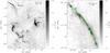 |
Fig. 1 Left: dust extinction map of the Chamaeleon-Musca region, based on 2MASS data (Kainulainen et al. 2009). Right: zoom-in to the Musca cloud, showing the instrument footprints of the observations employed in this work: NEWFIRM/NIR data (red rectangles), LABOCA/870 μm continuum emission (blue dashed lines, approximate coverage), SHeFI/C18O line emission (green crosses, from Hacar et al. 2016). |
One key open question related to filaments is whether: i) the filaments are close to hydrostatic objects prior to their fragmentation, in which case they first have to detach from the turbulent regime of the cloud and then fragment; or ii) the evolutionary picture of filaments is dynamic and hydrostatic conditions are never prevalent in the cloud. This question can be addressed by first carefully identifying filaments that are at the earliest stages of their evolution, possibly not yet fragmented, and by comparing their structure with the predictions of the hydrostatic equilibrium models. However in practice, doing this is severely hampered by the fact that nonfragmented filaments that carry the imprints of the initial condition are rare. This alone indicates that the phase in which a filament is nonfragmented and yet CO-emitting (so that it would be identified as a molecular cloud) is relatively short. While several recent works have made efforts to estimate the structure of filaments in nearby clouds (e.g., Arzoumanian et al. 2011; Fischera & Martin 2012b; Juvela et al. 2012b; Palmeirim et al. 2013), none of these works to our knowledge has identified and analyzed specifically nonfragmented filaments that would facilitate an assessment of the filament structure close to its initial condition.
Another key question is how the filaments fragment into dense cores that form stars. Analytic models predict the initially hydrostatic, infinitely long filament to fragment through gravitational instability at a wavelength of roughly four times the filament scale height (Inutsuka & Miyama 1992), in a timescale comparable to the sound-crossing time (order of a Myr, e.g., Fischera & Martin 2012a). For finite-sized filaments, it has been hypothezised that the local collapse timescale varies as a function of the position along the filament, and that the local collapse proceeds most rapidly at the ends of the filament (Bastien 1983; Pon et al. 2011). While testing these predictions is an active goal of observational studies (e.g., Jackson et al. 2010; Schmalzl et al. 2010; Busquet et al. 2013; Kainulainen et al. 2013; Takahashi et al. 2013), it is of great interest to find and characterize the fragmentation in filaments as simply as possible to isolate different processes that play a role.
Overview of NEWFIRM observations.
The main technical difficulty in addressing the questions above is the general difficulty of tracing the distribution of molecular gas in the ISM: all commonly-used tracers (dust emission, extinction, molecular line emission) have their specific problems and none of them can alone trace the wide range of column densities present in filaments. An additional difficulty is introduced by the small spatial scale of the filaments and their fragments. Filaments typically show widths that are on the order of 0.1 pc (e.g., Barnard 1927; Arzoumanian et al. 2011); fragments are similar in size. Consequently, single-dish observations can only study the structure of filaments in adequate detail in the most nearby molecular clouds (distances ≲200 pc). As a result, it remains unknown what the physical structure of filaments is like prior to their fragmentation and how exactly their fragmentation proceeds from that initial state to star formation.
To make progress in characterizing the early evolution and fragmentation of filaments, we target in this study the remarkably long (~6.5 pc), highly rectilinear Musca molecular cloud. The cloud is located in the Musca-Chamaeleon cloud complex (see Fig. 1) at the distance of ~150 pc (Knude & Hog 1998). The cloud has been identified to harbor only a very small number of cold cores given its spatial extent (Vilas-Boas et al. 1994; Juvela et al. 2010, 2011, 2012b), and it contains only one T Tauri star candidate, attesting to its current low star formation activity (Vilas-Boas et al. 1994). We have recently shown, using CO line observations, that Musca is entirely subsonic and velocity-coherent (Hacar et al. 2016). Contrasting this apparent quiescence, we have also shown that the probability distribution of column densities in the cloud shows a power-law-like excess of high-column densities, a feature common for star-forming molecular clouds (Kainulainen et al. 2009, 2011). Similarly, the cloud’s volume density distribution is more top heavy than that of other nearby starless clouds, suggesting that Musca may be close to active star formation (Kainulainen et al. 2014), or possibly in transition between non-star-forming and star-forming states.
The above properties make Musca a perfect candidate to be in the earliest phases of fragmentation. In this paper, we present a detailed study of the column density structure of Musca. We use archival near-infrared (NIR) observations and 870 μm dust emission observations to map column densities through the cloud and to characterize its internal structure. We then place the results in the context of hydrostatic equilibrium models, establish their suitability to describe the cloud, study its fragmentation, and finally propose an evolutionary scenario for the cloud.
2. Data and methods
2.1. NIR data and dust extinction mapping
The Musca cloud was observed with the NIR wide-field camera NEWFIRM (Autry et al. 2003) mounted on the Blanco 4-m telescope at the Cerro Tololo Inter-American Observatory between 2011 April 11 and 13. We retrieved the raw data and associated calibration files from the NOAO public archive. Six pointings (five covering the entire cloud and one off the cloud) were obtained in the J, H, and Ks broadband filters. Each pointing was observed in dither mode. Table 1 gives a summary of the observation strategy. We show the instrument footprints in Fig. 1, right panel; only four frames fall along the main part of Musca shown in the figure.
We processed the individual raw images using an updated version of Alambic (Vandame 2002), a software suite developed and optimized for the processing of large multi-CCD imagers. Alambic includes standard processing procedures, such as overscan and bias subtraction, flat-field correction, bad pixel masking, CCD-to-CCD gain harmonization, sky subtraction, and destripping. Aperture and PSF photometry were extracted from the individual images using SExtractor (Bertin & Arnouts 1996) and PSFEx (Bertin 2011). The individual catalogs were then astrometrically registered and aligned on the same photometric scale using Scamp (Bertin 2006), and the final mosaic produced using SWarp (Bertin et al. 2002). The photometric zero-points of the merged catalog were derived using the Two Micron All-Sky Survey (2MASS) catalog. The final absolute astrometric accuracy is expected to be better than 0.̋1 and the absolute photometric accuracy (rms of the individual images zeropoints) of the order of 5%. The NEWFIRM data were complemented with J, H, and Ks-band photometric data from the 2MASS archive (Skrutskie et al. 2006) to cover a wider field toward Musca. The area covered by the NEWFIRM frames cover the area used in all of our analyses; the 2MASS data is merely used to complete the outskirts of a wide-field extinction map (Fig. 1, right panel).
We used the JHKS-band data in conjunction with the nicest color-excess mapping technique (Lombardi 2009) to estimate the dust extinction through the Musca cloud. For the details of the technique, we refer to Lombardi (2009). The technique is based on comparing NIR colors (H−K and J−H) and surface density of the stars that shine through the cloud to those from a field that is assumed to be free from extinction. Since the photometric depths of the NEWFIRM and 2MASS data are different, these parameters were determined separately for the two data sets. In implementing nicest, a relative extinction law between JHKs-bands has to be assumed. We chose the empirical extinction law of Cardelli et al. (1989), i.e.,  (1)We emphasize that the technique estimates the dust extinction in NIR. We convert the estimates of NIR extinction to visual extinction by adopting the ratio between optical depths in NIR and visual wavelengths (Cardelli et al. 1989),
  (2)The visual extinctions are finally used to estimate the total hydrogen (atomic + molecular) column densities using the ratio measured by Savage et al. (1977) and Bohlin et al. (1978, see also Vuong et al. 2003; Güver & Özel 2009), i.e.,
  (3)The final extinction map of Musca is presented in Fig. 2, with higher detail blowups shown in Fig. 3. The map has the resolution of 45 arcsec and uncertainty at low column densities of σ(AV) = 0.2 mag. We analyze the column and volume density structure of the cloud, using this map, in Sects. 3.1 and 3.2.
2.2. LABOCA dust emission data
In addition to extinction maps, we carried out in May 2010 870 μm continuum observations of the Musca cloud using the LABOCA bolometric camera (Siringo et al. 2009) at the APEX telescope. The observations consisted of 14 individual raster-spiral maps combined to obtain a large-scale mosaic of approximately 2.2 by 0.4 deg2, covering the total extension of this cloud. Guided by our previous extinction maps of Musca (Kainulainen et al. 2009), the location, coverage, and overlap of these submaps were selected to optimize the sensitivity of the final mosaic along the main axis of the cloud. Skydips plus flux calibrations and pointing corrections in nearby sources were carried out every 1.5–2 h. Using the BoA software (Schuller 2012), the data reduction process followed the standard method described by Belloche et al. (2011) to recover the extended emission in the cloud. Convolved to a final resolution of 30 arcsec, the resulting map presents a typical rms of 17 mJy beam-1 and is shown in Fig. 2.
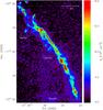 |
Fig. 2 Column density map of Musca (color scale), derived using NIR dust extinction mapping and data from NEWFIRM and 2MASS. The spatial resolution of the map is FWHM = 45″ and the sensitivity σ(NH) ≈ 0.4 × 1021 cm-2. The white boxes indicate three regions, which are shown in blowups in Fig. 3. The contours show the 870 μm continuum emission contours, observed with the APEX/LABOCA instrument and smoothed down to the resolution of the extinction data. The contours are drawn at the intervals of 0.03 mJy/beam, which is the 3σ rms noise of the smoothed data. |
 |
Fig. 3 Blowups from the NIR-derived column density map of the Musca cloud (Fig. 2). The contours start at NH = 1.5 × 1021 cm-2 and the step is 1.5 × 1021 cm-2. The lowest contour is drawn with a dotted line. The dashed lines in the Center region indicate the 1.6 pc velocity-coherent filament whose radial structure is modeled in Sect. 3.2. The numbered signs refer to the fragments identified within the cloud (see Sect. 3.1). |
2.3. SHeFI 13CO and C18O line emission data
We employ in the discussion of this paper 13CO (J = 2−1) and C18O (J = 2−1) line emission data of the Musca cloud from Hacar et al. (2016), to which we refer for the description of the observations and data reduction. The data were gathered with the SHeFI instrument at the ESO/APEX telescope in Chile. The spatial resolution of the data is  and the velocity resolution 0.10 km s-1 or 0.17 km s-1 (the receiver backend was changed during the observations). The spectra typically have a main beam temperature rms of 0.14 K. Line emission was observed in 305 positions along a curve that approximately traces the crest of the Musca cloud (see Fig. 1). The data were used to determine the central velocities, VLSR, and velocity dispersions, σv, along the filament. They were also used to estimate the nonthermal contributions to the observed line widths, σNT and σNT,corr (opacity-corrected), assuming a temperature of 10 K. For the details of the derivation of these values, we refer to Hacar et al. (2016).
3. Results
3.1. Column density structure of the Musca filament
Figure 2 shows the column density map of the Musca cloud derived from the NIR dust extinction data. Figure 3 shows zoom-ins of the map. The highest column densities in the map are about 35 × 1021 cm-2. The mean column density above 2 × 1021 cm-2 is ⟨ NH ⟩ = 4.5 × 1021 cm-2. Figure 2 also shows the contours of the LABOCA 870 μm emission data. The emission contours show good morphological correspondence with the NIR-derived column density map, evidencing that no column density peaks remain undetected from the NIR-derived data, e.g., because of the saturation of extinction or resolution effects. In general, the relationship between the extinction- and emission-derived column densities shows a high scatter, likely due to the spatial filtering of the dust emission data and their lower signal-to-noise ratio compared to extinction data; the relationship is presented in Appendix A.
We estimated the total mass of the cloud from the NIR-derived column densities by summing up all column densities inside the contours1 of NH = { 1.5,3,4.5 } × 1021 cm-2 (see Fig. 3 for the contours). This resulted in the total masses of M = { 281,174,132 } M⊙. We used the total masses to calculate equivalent2 line masses,  , of the entire Musca cloud. The length of Musca for all thresholds is about l = 6.5 pc, resulting in
  pc-1. The inclination angle, i, of the cloud is not known, and for reference, we adopt here i = 0. The inclination affects the line masses through a factor of cosi, and hence, the values we give represent upper limits. In addition to the inclination uncertainty, the uncertainty of the line mass is significantly affected by distance uncertainty, which is at least some ~10%.
Physical properties of fragments in Musca.
The column density map (Fig. 2) reveals numerous details within the large-scale Musca cloud. We divided the cloud into three regions, namely South, Center, and North, based on their morphology. The detailed column density maps of these regions are shown in Fig. 3.
The column density map (and emission data) show that Musca contains several small-scale condensations. For a simple, quantitative census of these structures, we identify “fragments” in the observed region. We emphasize that our purpose here is merely to have a first look at the small-scale substructures in the cloud; a simple fragment definition suffices for this purpose. With this in mind, we first smooth the resolution of the emission data down to the resolution of the extinction data (45′′) and identify fragment candidates as local emission maxima. In identifying the local maxima, we use contour steps of 0.03 mJy. If the fragment candidate is smaller than 45″ in diameter, it is rejected. As a second step, the fragment candidates are inspected against the local maxima of the extinction map. Local maxima are determined from the extinction data using contour intervals of 1.5 × 1021 cm-2. If the lowest contour that outlines a fragment candidate does not overlap with the lowest contour outlining an extinction maximum, the candidate is rejected. The pixel with maximum emission value is recorded as the location of the fragment. As a result of these steps, our fragments are essentially local emission maxima that have counterparts in the extinction map. The procedure results in identifying 21 fragments from the observed area.
We estimated the masses associated with the fragments by summing up all column densities from the NIR-derived data within circular apertures. The radii of the apertures, listed in Table 2, were chosen by eye. The fragment masses span 0.3–7.1 M⊙ (Table 2). We note that all column densities within the apertures were included in the calculation, i.e., possible “background” was not considered; it is not our goal to analyze the internal structure of the fragments or their relation to their surroundings. Finally, we roughly estimated the mean densities of the fragments from their area and mass, assuming spherical symmetry (Table 2).
In the following, we describe the specific properties of the South, Center, and North regions separately. The South region is clearly fragmented into five core-like structures, the most massive of which contain several solar masses. We measured the separation between the fragments as distances between neighboring fragments; in case of the South (and Center) this is trivial because the fragments are arranged into a line along the filament crest. The mean separation in South is 0.78 ± 0.6 pc. Note that the mean is strongly affected by the long distance between fragments #3 and 4; without the separation between those two fragments, the mean peak separation is 0.50 ± 0.2 pc. The total mass of the South region above NH = { 1.5,3,4.5 } × 1021 cm-2 are M = { 96,88,74 } M⊙. The region is about 2.7 pc long, resulting in the equivalent line masses of  pc-1. Finally, we note that fragments #4 and #5 practically compose the object studied as “a filament” by Juvela et al. (2012b). It appears to us that this region is clearly fragmented, and therefore, the axisymmetric cuts across the region measure in effect a combination of the profile of the fragments and that of the collapsing filament, not the profile of the filament itself.
The Center region of the Musca cloud consists of a 1.6 pc long filament, which shows less substructure than the South region and has a relatively constant peak column density of NH ≈ 10−15 × 1021 cm-2 along its crest. The line mass of this filament using the column density thresholds of NH = { 1.5,3,4.5 } × 1021 cm-2 results in Ml = { 31,26,21 } M⊙ pc-1. Thus, its line mass is practically the same as that of the entire Musca cloud on average and that of the South and North (see below) regions. The FWHM of the filament is 0.07 pc, measured from its mean column density profile (see Sect. 3.2). There are five fragments along the main filament and one about 0.5 pc off the filament. The fragments along the filament have very low contrast to their surroundings compared to those in the South (see the quantification of the column density contrast later in this section). The mean separation of the five fragments along the crest is 0.35 ± 0.13 pc (fragment #9 was not included in the analysis). We consider physical models for the Center filament in Sect. 3.2.
The North region of the Musca cloud is clearly fragmented, similar to the South region. In the southwest corner of the region, there is a complex area containing four fragments. This region is characterized by two velocity components, likely resulting from two overlapping structures (Hacar et al. 2016). In the middle of the North region, there is a curious structure, which consists of two thin (NH ≈ 3 × 1021 cm-2) structures parallel to each other (a bubble-like structure), and of two peaks (fragments #19 in the northwest and fragments #17 and 18 in the southeast) that are elongated almost in perpendicular direction to those two structures. Unfortunately, we did not cover this region with molecular line data, and thus the nature of the structure remains unclear. There is a strong local maximum at the northeast corner of the region. This peak coincides with the location of the only candidate young star (T Tauri star candidate, Vilas-Boas et al. 1994) in the cloud. The North region harbors ten fragments (Table 2). These fragments are not aligned along a line as clearly as fragments in the Center and South regions. Acknowledging this caveat, we calculated the separations along two routes that connect the fragments (in the order of the fragment number): one including fragment #19 and excluding fragments #17 and 18, and the other excluding fragment #19 and including fragments #17 and 18. This resulted in mean separations of 0.24 ± 0.16 pc and 0.25 ± 0.17 pc, respectively. The total masses of the region above NH = { 1.5,3,4.5 } × 1021 cm-2 are M = { 59,47,37 } M⊙. With the approximate length of 2.0 pc of the region, these result in the equivalent line masses of  pc-1.
pc-1.
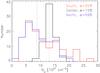 |
Fig. 4 Frequency distribution of column density values along the approximate crest of the Musca cloud for South (red), Center (black), and North (blue) regions. The dashed lines indicate the mean column densities. The relative standard deviation of the column density values in each region is shown in the panel. |
We emphasize that the North and South regions contain high-contrast density enhancements compared to the smoother, filamentary Center region; even though we identify “fragments” from the Center region, their column density contrast against their surrounding, more elongated gas component is very low. We further quantify this morphological difference by measuring the standard deviation of column density (extinction) values along the approximate crest of the cloud (see Fig. 1 right panel). The histograms of the extinction values along the crest in different regions are shown in Fig. 4. The figure shows that the distributions of the North and South regions are clearly different from that of the Center region: the North and South peak at around NH ≈ 6 × 1021 cm-2 and have strongly skewed distributions, while the Center peaks at around NH ≈ 13 × 1021 cm-2 and has a narrow distribution. The relative standard deviations of the extinction values along the cloud crest are: 55% for South, 49% for North, and 15% for the Center. This shows that the column density variation in the Center is clearly smaller, by a factor of ~3, than in the North and South.
3.2. Physical models for the Center filament
The column density maps of the Center region (Figs. 2, 3) revealed an about 1.6 pc long, relatively nonfragmented filament. In this section, we examine the radial structure of this filament and consider physical models for it.
We estimated the mean column density profile of the Center filament from radial cuts across it. For this purpose, we first defined the filament crest by connecting the local maxima within the NH = 8 × 1021 cm-2 contour with lines. The filament crest is shown in Fig. A.1 and the points defining it are given in Table B.1. We then sampled the radial profile with cuts perpendicular to the crest. The positions of the cuts along the crest were separated by 4 pixels to ensure that the profiles at the crest position are not correlated. Consequently, the 1.6 pc long filament was sampled with 20 profiles.
Figure 5 shows the resulting mean profiles, given separately for the west and east sides of the filament. Importantly, the profiles show that the filament is not symmetric, but the west side of it is steeper than the east side. The CO spectra show two velocity components on the east side of the filament crest (cf. Hacar et al. 2016), suggesting that another, faint structure overlaps with the main crest at the east side. This asymmetry is also seen at larger scales in the extinction map of the region (see Fig. 1). Therefore, we consider that the west side profile reflects the true filament profile more correctly. It is noteworthy that even if Musca seems to represent one of the simplest filamentary clouds we know, its radial profile is asymmetric with respect to the main axis when resolved in high detail. Similarly, as shown in Sect. 3.1, small scale variations are present even in the simple Musca filament. These phenomena are likely present in more complex filamentary clouds, such as L1495-B213 (e.g., Schmalzl et al. 2010) and IC 5146 (e.g., Arzoumanian et al. 2011). Our observations suggest caution when analyzing profiles of complex filaments by averaging individual profiles and need to be addressed for the correct physical interpretation of the derived parameters. In the following, we quantify the radial structure of the Center filament in Musca by fitting different physically motivated models to its observed profile.
3.2.1. Isolated, infinite filament in hydrostatic equilibrium
We first modeled the 1.6 pc long filament in the Center region in the context of an infinite, isolated cylinder in equilibrium between thermal and gravitational pressures (Ostriker 1964). This kind of an equilibrium configuration has the line mass,  (4)where cs is the sound speed. This indeed is close to the observed line mass of the Center filament (Ml = 21−31 M⊙). It is possible that nonthermal motions provide additional support for a filament, making its critical line mass higher. An estimate of this “turbulent support” can be calculated from Eq. (4) by replacing the sound speed with an effective sound speed, cs,eff, which results from the total line width in the cloud. The nonthermal line width of C18O) is about 0.7cs, yielding
  . The critical line mass is affected by the square of this, yielding 24 M⊙ pc-1.
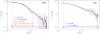 |
Fig. 5 Mean radial column density profiles along the Center filament of the Musca cloud. The left and right panels show the mean profile on the west and east sides of the filament axis, respectively. The blue line shows the fit of Plummer-like profile, and red line shows the fit of a pressure-confined hydrostatic cylinder. The colored arrows indicate the radial ranges used in fitting the profiles. The error bars show the standard deviation of 20 individual profiles from which the mean profile is constructed. The vertical dashed line shows the FWHM size of the extinction mapping beam. |
Parameters of the best-fit radial density distribution models.
The volume density profile of the infinite, hydrostatic filament in equilibrium is (Ostriker 1964)  (5)where r0 is the scale radius as defined by Ostriker (1964), ρc the central density, and the exponent p = 4. If the exponent is not 4, the radial profile does not describe an equilibrium solution. Using the generic, Plummer-like profile is useful, however, because it allows for quantification of r0, ρc, and p through a fit to an observed profile, and from therein, examination of the validity of the model. The scale radius is coupled to the central density and temperature, T, through
  (6)The column density profile corresponding to the volume density profile is (e.g., Arzoumanian et al. 2011)
  (7)In the equation,
  , with i as the inclination angle of the filament, which we assume to be zero.
Figure 5 shows the best fit of Eq. (7) to the observed mean profile, achieved by treating ρc, r0, and p as free parameters, fixing the fitting range to r = [0,0.6] pc, and then minimizing the chi-square between the data points and the model. The inverse variances of the 20 individual profile cuts were used as the weights of the data points in the fit. The best-fit model for the west-side profile has the exponent p = 2.6 ± 11%, the scale radius r0 = 0.016 ± 33% pc, and the central density nc = 54 000 ± 50% cm-3 (Table 3). The quoted errors are the one-sigma uncertainties of the fit. One should note that fitting Eq. (7) in this manner suffers from degeneracy between ρc, r0, and p (Juvela et al. 2012a; Smith et al. 2014). This degeneracy likely causes the large uncertainties in r0 and ρc. The slope p suffers less from the degeneracy and in general can be constrained with lower uncertainty (Smith et al. 2014).
3.2.2. Isothermal filament in equilibrium, confined by external pressure
We also modeled the filament in the Center region as a pressure-confined (and truncated), isothermal filament in hydrostatic equilibrium (Fischera & Martin 2012a). The column density profile of this model is ![Mathematical equation: \begin{eqnarray} N (x) & = & \sqrt{\frac{p_\mathrm{ext}}{4 \pi G}} \frac{\sqrt{8}}{1-f_\mathrm{cyl}} (\mu m_\mathrm{H})^{-1} \nonumber \\ & & \times \frac{1-f_\mathrm{cyl}}{1-f_\mathrm{cyl} + x^2f_\mathrm{cyl}} \left[\sqrt{ f_\mathrm{cyl}(1-f_\mathrm{cyl})(1-x^2 ) } \phantom{\sqrt{ \frac{(x_\mathrm{cyl}^2)}{(x^2)} } } \nonumber\right. \\ & & \left.+ \sqrt{ \frac{1-f_\mathrm{cyl}}{1-f_\mathrm{cyl}(1-x^2)} } \times \arctan{ \sqrt{ \frac{f_\mathrm{cyl}(1-x^2)}{1-f_\mathrm{cyl}(1-x^2)} } } \right]\cdot \label{eq:fischera} \end{eqnarray}](/articles/aa/full_html/2016/02/aa26017-15/aa26017-15-eq110.png) (8)In this equation, the dimensionless coordinate x is the radius, r, normalized by the outer radius of the filament, Rf, i.e., x = r/Rf, and fcyl = Ml/Ml,crit is the ratio of the filament’s line mass to the critical line mass, (see Eq. (4) for Ml,crit). The relative shape of the column density profile depends only on the parameter fcyl and on the normalization of the radial profile, i.e., on Rf. The temperature and line mass affect the profile shape implicitly through fcyl. In addition, the normalization of the profile is affected by the confining external pressure pext.
(8)In this equation, the dimensionless coordinate x is the radius, r, normalized by the outer radius of the filament, Rf, i.e., x = r/Rf, and fcyl = Ml/Ml,crit is the ratio of the filament’s line mass to the critical line mass, (see Eq. (4) for Ml,crit). The relative shape of the column density profile depends only on the parameter fcyl and on the normalization of the radial profile, i.e., on Rf. The temperature and line mass affect the profile shape implicitly through fcyl. In addition, the normalization of the profile is affected by the confining external pressure pext.
The applicability of this model can be immediately examined through fcyl, which in the context of this model cannot be larger than unity. In Sect. 3.1, we estimated the line mass of the filament to be Ml = { 31,26,21 } M⊙ when using the column density thresholds of NH = { 1.5,3,4.5 } × 1021 cm-2 to compute the line mass. The critical line mass without the contribution from nonthermal motions (16 M⊙ pc-1) is slightly below this range, and the critical line mass with the nonthermal contribution (24 M⊙ pc-1) overlaps with it. One should note that the observed line masses are upper limits because of the assumption of zero inclination. Distance uncertainty is also at least some 10%. We also do not know exactly the temperature structure of the filament, which also affects Ml,crit. Finally, in the context of this model, the filament is pressure confined by the surrounding gas; this surrounding gas possibly contributes to the observed Ml value (we address this further below). We conclude that the observed line masses are such that considering the pressure-confined filament model is reasonable.
We fitted Eq. (8) to the observed data points at radii below 0.6 pc by letting fcyl and pext change as free parameters, again using the inverse variances of the 20 profiles to weight the data points. This did not yield an acceptable fit. However, also allowing the fitting radius, i.e., the radius of the filament, to change as a free parameter and ignoring the profile outside it resulted in a reasonable fit (see Fig. 5). The best fit has the parameters fcyl = 0.66 ± 12%, and pext = 12 ± 37% × 104 K cm-3, and Rf = 0.12 ± 7% pc where the uncertainties result from the chi-square fit (Table 3). The external pressure is consistent with pressures needed to confine isolated globules modeled as Bonnor-Ebert spheres (~2–20 × 104 K cm-3, Kandori et al. 2005), and a factor of a couple higher than inferred for parsec-scale filaments (~1–5 × 10⁴ K cm-3, Fischera & Martin 2012a,b).
One has to recognize that the above model does not include any contribution to the observed column densities from the surrounding gas, which is required to provide the confining pressure (see the discussion in Recchi et al. 2014). Thus, the use of Eq. (8) by itself may not be physically entirely meaningful. In practice, the confining pressure could arise from the thermal pressure in a two-phase medium, in which the cooler, denser component is surrounded (and confined) by the less dense, warm component. Accretion of gas into the filament could also possibly provide confining pressure (Heitsch 2013a,b). Turbulent ram pressure could also provide confining pressure, although to provide confinement, it should be relatively isotropic, which may be unrealistic. Regardless of the nature of the pressure, a surrounding gas component is needed, and can affect the observed column density structure.
To explore the effect of the surrounding gas to the parameters of this model, we made an experiment in which the pressure-confined filament is embedded inside a cylindric envelope (e.g., Hernandez et al. 2012; Recchi et al. 2014). This cylindric envelope has a power-law radial density distribution, ρe(r) = Cr-2, where C is a proportionality constant. The column density profile of the envelope results then from integrating ρe(r) along the line of sight (see, e.g., Recchi et al. 2014), yielding  (9)where Re and Rf are the radius of the envelope and filament, respectively. At the limit r → 0, the equation has the value
  , which gives the column density of the envelope at r = 0, i.e., N0. The total column density of the model is the sum of the envelope and the embedded filament (Eq. (8)). This model was fitted to the observed profile with fcyl, pext, Rf, and C as free parameters, assuming that the envelope goes to zero at 0.6 pc, i.e., Re = 0.6 pc (Fig. 6). We stress here that our goal is to probe how the filament parameters are affected by an envelope, not to find the best possible envelope model, nor even a physically meaningful one. It is evident that the envelope model we use is rather arbitrary, and other envelopes may well produce equally good fits.
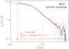 |
Fig. 6 Mean radial column density profiles along the Center filament. The red line shows the fit of a pressure-confined equilibrium model (Fischera & Martin 2012a), embedded inside a cylindric envelope. The black dashed line shows the column density profile of the filament without the surrounding envelope. The dashed vertical line shows the FWHM size of extinction mapping beam. |
We find that the observed profile is best fit when a filament is surrounded by an envelope that has the central column density N0 = 2.4 × 1021 cm-2. The parameters of the embedded filament, i.e., fcyl and pext (see Table 3) are not significantly different from those of the filament without the envelope. In conclusion, a pressure-confined hydrostatic filament, embedded in a low-density envelope, seems to provide a reasonable explanation for the entire observed column density profile.
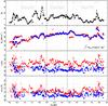 |
Fig. 7 Column density and velocity structure of Musca, measured approximately along the crest of the cloud (see Fig. 1). The top panel shows the dust extinction from NIR data. The second panel shows the central velocities, Vlsr. The third and bottom panels show the nonthermal velocity dispersions, σNT (noncorrected) and σNT,corr (opacity-corrected), normalized by the sound speed cs. The arrows in the bottom panel indicate upper limits. The red and blue points show the data for 13CO (2–1) and C18O (2–1), respectively. The locations of the fragments, which are closer than 100 arcsec of the cloud crest, are indicated with thin dashed lines. The thick dashed vertical lines separate the South, Center, and North regions from each other. The thick dashed horizontal line indicates the sonic velocity dispersion, and the dotted horizontal line the two times is the sonic velocity dispersion. The lower right corner of the middle panel indicates with a line a velocity gradient of 3 km s-1. The figure is a reproduction from Hacar et al. (2016). |
3.3. Relationship between the column density and velocity structure in Musca
We briefly compare in this section the column density structure of the Musca cloud to the large-scale kinematic data from Hacar et al. (2016). While Hacar et al. discusses the properties of the global velocity field in Musca, we consider here those data in the context of the column density structure and fragments of the cloud.
Figure 7 shows the NIR-derived column densities, 13CO and C18O central velocities (Vlsr), nonthermal velocity dispersions (σNT), and nonthermal opacity-corrected velocity dispersions (σNT,corr) for the ~300 line of sights observed along the Musca cloud (see Fig. 1). There are some double-peaked spectra at the edges of the cloud; Fig. 7 shows the Vlsr and σNT values for both these components, obtained via fits of separate Gaussian components (see Hacar et al. 2016, for details). The locations of the fragments, which are closer than 100 arcsec of the cloud crest, are also shown in the figure. As found out by Hacar et al. (2016), Musca is velocity-coherent and subsonic at densities probed by the C18O data (sub-/transsonic at densities probed by the 13CO data) practically throughout its length. The velocity gradient along the South region is about dVlsr/ dr ≈ 0.5 km s-1 pc-1. The South region also shows local velocity gradients, up to ~3 km s-1 (cf. Hacar et al. 2016), which clearly coincide with the column density fragments. The North and Center regions show a velocity gradient of dVlsr/ dr ≈ 0.15 km s-1 pc-1, with the only local gradients coinciding with the densest fragment in the North region (#21) and the complex clump of multiple maxima (close to fragment #13). In particular, the two most pronounced fragments in the Center region (#6 and 7 in Table 2) do not show gradients in C18O central velocities. The scatter of the line velocities in the North and South is clearly larger than in the Center (dominantly due to the large-scale gradient): σ(VLSR,C18O)south = 2.03 km s-1, σ(VLSR,C18O)center = 0.67 km s-1, σ(VLSR,C18O)north = 1.57 km s-1. The North and South also show slightly larger scatter of nonthermal velocity dispersions than the Center: σ(σNT,C18O)south = 0.3 km s-1, σ(σNT,C18O)center = 0.2 km s-1, σ(σNT,C18O)north = 0.24 km s-1. Finally, some oscillatory motions are seen at the locations of the two most prominent fragments in the South region (#4 and 5). Their presence suggests that fragmenting modes indeed are present in the cloud (cf. Hacar & Tafalla 2011).
Summarizing, the above properties demonstrate the fact that even if Musca as a whole is subsonic and velocity coherent, the opposite ends of it show slightly more active internal dynamics than the extremely quiescent Center filament. This activity is likely related to the fragments present at the ends of the cloud.
4. Discussion
4.1. Musca: caught in the middle of gravitational fragmentation
What do our observations tell us about the nature of Musca and its fragmentation? We have demonstrated that the physical structure of the extremely quiescent Center filament of Musca is in a good agreement with the predictions for the line mass, radial density distribution, and velocity structure of the pressure-confined hydrostatic equilibrium model. The cloud contains 21 fragments (according to our definition of fragments), with the higher-contrast fragments located in the South and North regions. Specifically, the North and South have a factor of three higher column density variance compared to the Center region. Some of the fragments contain several solar masses, and thus have the potential to be prestellar cores. Importantly, the equivalent line masses of the North and South are equal with the line mass of the Center filament, giving rise to a hypothesis that they may have fragmented from an initial condition that resembles the relatively nonstructured Center filament.
To further examine this hypothesis, we consider the prediction of the gravitational fragmentation model (the pressure-confined filament, Fischera & Martin 2012a) for the fragmentation length and timescale of a cylinder that has the properties of the Center filament. In this model, filaments with line masses less than the critical line mass can fragment when perturbed. Filaments with line masses larger than critical (that are not equilibrium solutions to begin with) should collapse into a spindle rapidly. The wavelength of the fastest growing perturbations is between λm = 5−6.3 × FWHMcyl (Fischera & Martin 2012a). The lower limit corresponds to the case fcyl → 1 and the upper limit to fcyl → 0. We measured the FWHM of the Center filament to be 0.07 pc, which results in the fragmentation scale of λm ≈ 0.35−0.44 pc. The observed mean peak separation of the fragments in all regions is 0.41 ± 0.37 pc and the median is 0.34 pc (mean is 0.32 ± 0.18 pc and median 0.33 pc without the long separation between fragments #3 and 4), overlapping with the predicted interval. The results are practically the same regardless of how we compute the separations in the North region (see Sect. 3.1). Fragment #9 is not included in this analysis because of its location off the filament axis. In conclusion, it appears that also from point of view of the fragmentation scale, the North and South regions may have originated from an initial condition that resembles the Center filament.
The fragmentation timescale of the infinite, pressure-confined cylinder depends on fcyl, T, and pext (Fischera & Martin 2012a), and is between 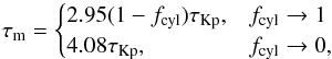 (10)where
 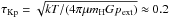 Myr. This gives the range τm ≈ 0.2−0.8 Myr when using the parameters of the best-fitting pressure-confined model (Table 3). We note the caveat that the above predictions for the fragmentation scale and timescale are for infinite cylinders; it may be that the predictions differ in finite geometry.
Why has the fragmentation proceeded strongly at the ends of the Musca cloud, but not at its center? One possible mechanism in the context of gravitational fragmentation is provided by finite-size effects in cylindric geometry (as opposed to the infinite models of Ostriker 1964; and Fischera & Martin 2012a). In finite filaments, the acceleration of gas depends on the relative position along the filament, which is largest at its ends (Bastien 1983; Pon et al. 2011, 2012; Clarke & Whitworth 2015, see also Burkert & Hartmann 2004, for a study in a sheet geometry). These higher accelerations may translate into shorter local collapse timescales, and therefore, into formation of fragments at the ends of the filament prior to its center (Pon et al. 2011, 2012). For example, Pon et al. (2011, see their Figs. 5 and 6) suggest that the local collapse might occur a factor of two-to-three faster at the ends of the filament than at its center. Similarly, Clarke & Whitworth (2015) found in their numerical simulations that the first fragments form at the ends of the filament, regardless of its aspect ratio. While there are some quantitative differences between the predictions of Clarke & Whitworth (2015) and Pon et al. (2011, 2012), both models predict that long (but finite-sized) filaments fragment starting from the ends of the cloud. Consequently, they lay out the basis for explaining the fragmentation at the ends of Musca as a result of the end-dominated collapse caused by higher accelerations, and therefore, shorter local collapse timescales.
In the models of Pon et al. (2011, 2012) and Clarke & Whitworth (2015), high-aspect ratio filaments collapse globally and the fragments formed at the ends of the cloud fall into its centre; this can be used to gain further insight into the evolution of Musca under this framework. The timescales for the global collapse (timescale for the end fragments to reach the cloud centre) are (following the notation of Clarke & Whitworth 2015) (11)and
  (12)where G is the gravitational constant and ρ0 the central density. The aspect ratio of Musca depends on how we define its width. If we adopt the ~0.6 pc extent of the Plummer profile (see Fig. 5), the aspect ratio 6.5 pc/0.6 pc ≈ 5 follows; if we adopt the 0.1 pc radius of the pressure-confined filament, the aspect ratio is 6.5 pc/0.2 pc ≈ 32. This interval of A = 5−33 is very conservative, as it represents the extreme choices for the filament width. For the central density, we use 105 cm-3. The global collapse timescale for the chosen range of aspect ratios is then between ~0.5–3 Myr, depending on the model. We showed earlier that the fragmentation timescale of an infinite pressure-confined filament is between 0.2–0.8 Myr. Even if these estimates are highly uncertain, they suggest that the fragmentation timescale may be significantly shorter than the global collapse timescale. This is in agreement with the fact that we do not observe Musca to be globally collapsing, but rather forming multiple fragments along it. This, in turn, suggests that the age of Musca is rather closer to its fragmentation timescale than its global collapse timescale, i.e., only some tenths of a Myr. Alternatively, additional processes must be supporting Musca against global collapse.
Instead of the gravitational focusing, another possibile way to explain the differences in fragmentation along Musca may be differences in the initial physical properties along the cloud. In principle, the fragmentation timescale anticorrelates with the line mass (e.g., Fischera & Martin 2012a); however, as shown earlier, the equivalent line masses of the North and South are the same as the line mass of the Center, stating that they should collapse in the same timescale. It could also be hypothesised that difference in the dynamics of the regions plays a role: the North and South regions show significantly higher global velocity gradients than the Center region, which might affect fragmentation in the North and South regions. Whether this kind of an initial velocity gradient could promote fragmentation remains to be explored via theoretical works. Finally, the timescale also correlates with the size of the initial density perturbations (Pon et al. 2011). It cannot be ruled out that the North and South regions would have had higher density variance along them compared to the Center, inducing faster fragmentation.
Ultimately, one would like to compare the timescales derived above with other age estimators in the cloud. However, the only direct signpost of age in Musca is the single T Tauri star candidate in the North region (fragment #21). Its presence indicates that fragmentation in the North region (and supposedly in South) must have taken place on the order of ~0.5 Myr ago (Class 0+1 protostellar lifetime, Dunham et al. 2014), with an admittedly large uncertainty. We showed earlier that the timescale of gravitational fragmentation in Musca is 0.2–0.8 Myr, coinciding with this estimate. Further studies targeting, e.g., the chemical ages at the different locations along the filament would provide additional, independent measures of age.
Altogether, the morphology of Musca, its fragmentation, radial structure, and velocity characteristics suggest that gravitational fragmentation is taking place in situ in Musca, molding it toward star formation. This is in a qualitative agreement with our earlier results regarding the cloud’s column density structure: in Kainulainen et al. (2009) we analyzed the probability density function of column densities (N-PDF) in Musca, showing that it exhibits (at least a start of) a power-law-like tail at high-column densities, similar to actively star-forming clouds. Further, in Kainulainen et al. (2014) we showed, with the help of volume density modeling, that Musca currently contains only a very small amount of gas (~6 M⊙) at densities high enough for star formation. From the point of view of its column and volume density structure, the cloud must become more condensed locally to form stars; this could happen via the ongoing fragmentation and gravitational collapse. Musca represents a perfect target for studying this: the simplicity of the cloud is ideal for isolating the different processes driving fragmentation.
5. Conclusions
We analyzed the column density structure and fragmentation of the 6.5 pc long, rectilinear Musca molecular cloud, which shows very little sign of ongoing star formation. We examined the structure of the cloud with the help of NIR dust extinction data and 870 μm dust emission data. We also examined the large-scale kinematic structure of Musca using 13CO and C18O line emission data (from Hacar et al. 2016). Our conclusions are as follows:
-
1.
The column density data show that the Musca cloud isfragmented into 21 fragments that have massesbetween ~0.3–7 M⊙. The Center regionof Musca harbors a remarkably well-defined, 1.6 pc long filamentthat contains only low-contrast fragments. The filament showsonly 15% relative column density variations along its crest, instark contrast to ~50% variations in the more pronouncedly fragmented ends of the cloud. We emphasize that the relative column density variations provide a physically motivated, simple measure of how fragmented a filament is; a low degree of fragmentation is necessary for characterizing the initial condition of fragmenting filaments.
-
2.
The line mass of the Center filament is 21–31 M⊙ pc-1, i.e., close to the critical value of a cylinder in hydrostatic equilibrium. The equivalent line masses (total mass divided by length) of the North and South regions are practically the same.
-
3.
The radial density structure of the Center filament is well described with either i) a Plummer profile that has a power-law exponent of 2.6, scale radius of 0.016 pc (FWHM of 0.07 pc), and central density of 5 × 104 cm-3; or ii) a hydrostatic filament that is confined by external pressure imposed by a surrounding envelope. In this case the ratio of the line mass to the critical line mass is 0.66, central density is 105 cm-3, and external pressure is ~105 K cm-3. We note that even this simple and well-resolved filament shows an asymmetric column density profile with respect to the main filament axis. This suggests caution when analyzing profiles of filaments that are more complicated than Musca.
-
4.
The fragmentation length of the cloud, ~0.4 pc, agrees with the prediction of the gravitational fragmentation of an infinite, pressure-confined cylinder. The fragmentation timescale predicted by the model is 0.2–0.8 Myr and the global collapse time of the cloud 0.5–3 Myr.
-
5.
The ends of Musca show somewhat more variation in their C18O velocity structure than the extremely quiescent Center region, both in the central line velocities and the scatter of nonthermal line widths. The central line velocities peak at the locations of the fragments, suggesting motions associated with the fragments.
The above characteristics give rise to a hypothesis for the evolutionary scenario of Musca: an initially 6.5 pc long, close-to hydrostatic filament is in the middle of gravitational fragmentation. Fragmentation started a few tenths of a Myr ago, and it has so far taken place only at the ends of the cloud, possibly because of the shorter local collapse timescales compared to the cloud center (“gravitational focusing”). The relatively nonfragmented Center region may still represent the close-to hydrostatic initial condition of the filament, regardless of whether the fragmentation at the ends of the cloud is driven by gravitational focusing or some other process.
To describe how the chosen contour level affects the results, we give the masses and line masses corresponding to three different contour levels.
We use the term “equivalent line mass” because the cloud is partly fragmented (North and South regions) and does not resemble a well-defined filament throughout its length. In this case, “line mass” alone would be a somewhat misleading term.
Acknowledgments
The authors thank S. Recchi and F. Heitsch for valuable discussions, and the anonymous referee for constructive comments that improved the paper. The work of J.K. was supported by the Deutsche Forschungsgemeinschaft priority program 1573 (“Physics of the Interstellar Medium”). J.K. gratefully acknowledges support from the Finnish Academy of Science and Letters/Väisälä Foundation. H. Bouy is funded by the Ramón y Cajal fellowship program number RYC-2009-04497. This research has been funded by Spanish grants AYA2012-38897-C02-01. This publication makes use of data products from the Two Micron All Sky Survey, which is a joint project of the University of Massachusetts and the Infrared Processing and Analysis Center/California Institute of Technology, funded by the National Aeronautics and Space Administration and the National Science Foundation.
References
- André, P., Men’shchikov, A., Bontemps, S., et al. 2010, A&A, 518, L102 [NASA ADS] [CrossRef] [EDP Sciences] [Google Scholar]
- André, P., Di Francesco, J., Ward-Thompson, D., et al. 2014, Protostars and Planets VI, 27 [Google Scholar]
- Arzoumanian, D., André, P., Didelon, P., et al. 2011, A&A, 529, L6 [Google Scholar]
- Autry, R. G., Probst, R. G., Starr, B. M., et al. 2003, Proc. SPIE, 4841, 525 [Google Scholar]
- Bally, J., Lanber, W. D., Stark, A. A., & Wilson, R. W. 1987, ApJ, 312, L45 [NASA ADS] [CrossRef] [Google Scholar]
- Bastien, P. 1983, A&A, 119, 109 [NASA ADS] [Google Scholar]
- Barnard, E. E. A Photographic Atlas of Selected Regions of the Milky Way, eds. E. B. Frost, & M. R. Calvert (Washington: Carnegie Institution of Washington), 1927 [Google Scholar]
- Belloche, A., Schuller, F., Parise, B., et al. 2011, A&A, 527, A145 [NASA ADS] [CrossRef] [EDP Sciences] [Google Scholar]
- Bertin, E. 2006, Astronomical Data Analysis Software and Systems XV, 351, 112 [NASA ADS] [Google Scholar]
- Bertin, E. 2011, Astronomical Data Analysis Software and Systems XX, 442, 435 [NASA ADS] [Google Scholar]
- Bertin, E., & Arnouts, S. 1996, A&AS, 117, 393 [NASA ADS] [CrossRef] [EDP Sciences] [Google Scholar]
- Bertin, E., Mellier, Y., Radovich, M., et al. 2002, Astronomical Data Analysis Software and Systems XI, 281, 228 [NASA ADS] [Google Scholar]
- Bohlin, R. C., Savage, B. D., & Drake, J. F. 1978, ApJ, 224, 132 [NASA ADS] [CrossRef] [Google Scholar]
- Burkert, A., & Hartmann, L. 2004, ApJ, 616, 288 [NASA ADS] [CrossRef] [Google Scholar]
- Busquet, G., Zhang, Q., Palau, A., et al. 2013, ApJ, 764, L26 [NASA ADS] [CrossRef] [Google Scholar]
- Cardelli, J. A., Clayton, G. C., & Mathis, J. S. 1989, ApJ, 345, 245 [NASA ADS] [CrossRef] [Google Scholar]
- Clarke, S. D., & Whitworth, A. P. 2015, MNRAS, 449, 1819 [NASA ADS] [CrossRef] [Google Scholar]
- Dobashi, K., Uehara, H., Kandori, R., et al. 2005, PASJ, 57, 1 [Google Scholar]
- Dunham, M. M., Stutz, A. M., Allen, L. E., et al. 2014, Protostars and Planets VI, 195 [Google Scholar]
- Fiege, J. D., & Pudritz, R. E. 2000a, MNRAS, 311, 85 [NASA ADS] [CrossRef] [Google Scholar]
- Fiege, J. D., & Pudritz, R. E. 2000b, MNRAS, 311, 105 [NASA ADS] [CrossRef] [Google Scholar]
- Fischera, J., & Martin, P. G. 2012a, A&A, 542, A77 [NASA ADS] [CrossRef] [EDP Sciences] [Google Scholar]
- Fischera, J., & Martin, P. G. 2012b, A&A, 547, A86 [NASA ADS] [CrossRef] [EDP Sciences] [Google Scholar]
- Goodman, A. A., Alves, J., Beaumont, C. N., et al. 2014, ApJ, 797, 53 [NASA ADS] [CrossRef] [Google Scholar]
- Güver, T., & Özel, F. 2009, MNRAS, 400, 2050 [NASA ADS] [CrossRef] [Google Scholar]
- Hacar, A., & Tafalla, M. 2011, A&A, 533, A34 [NASA ADS] [CrossRef] [EDP Sciences] [Google Scholar]
- Hacar, A., Tafalla, M., Kauffmann, J., & Kovács, A. 2013, A&A, 554, A55 [NASA ADS] [CrossRef] [EDP Sciences] [Google Scholar]
- Hacar, A., Kainulainen, J., Beuther, H., Tafalla, M., Alves, J. 2016, A&A, in press, DOI: 10.1051/0004-6361/201526015 [Google Scholar]
- Hernandez, A. K., Tan, J. C., Kainulainen, J., et al. 2012, ApJ, 756, L13 [NASA ADS] [CrossRef] [Google Scholar]
- Heitsch, F. 2013a, ApJ, 769, 115 [NASA ADS] [CrossRef] [Google Scholar]
- Heitsch, F. 2013b, ApJ, 776, 62 [NASA ADS] [CrossRef] [Google Scholar]
- Hill, T., Motte, F., Didelon, P., et al. 2011, A&A, 533, A94 [NASA ADS] [CrossRef] [EDP Sciences] [Google Scholar]
- Inutsuka, S.-I., & Miyama, S. M. 1992, ApJ, 388, 392 [NASA ADS] [CrossRef] [Google Scholar]
- Inutsuka, S.-i., & Miyama, S. M. 1997, ApJ, 480, 681 [NASA ADS] [CrossRef] [Google Scholar]
- Jackson, J. M., Finn, S. C., Chambers, E. T., Rathborne, J. M., & Simon, R. 2010, ApJ, 719, L185 [NASA ADS] [CrossRef] [Google Scholar]
- Juvela, M., Ristorcelli, I., Montier, L. A., et al. 2010, A&A, 518, L93 [NASA ADS] [CrossRef] [EDP Sciences] [Google Scholar]
- Juvela, M., Ristorcelli, I., Pelkonen, V.-M., et al. 2011, A&A, 527, A111 [NASA ADS] [CrossRef] [EDP Sciences] [Google Scholar]
- Juvela, M., Malinen, J., & Lunttila, T. 2012a, A&A, 544, A141 [NASA ADS] [CrossRef] [EDP Sciences] [Google Scholar]
- Juvela, M., Ristorcelli, I., Pagani, L., et al. 2012b, A&A, 541, A12 [NASA ADS] [CrossRef] [EDP Sciences] [Google Scholar]
- Kainulainen, J., Beuther, H., Henning, T., & Plume, R. 2009, A&A, 508, L35 [NASA ADS] [CrossRef] [EDP Sciences] [Google Scholar]
- Kainulainen, J., Beuther, H., Banerjee, R., et al. 2011, A&A, 530, A64 [NASA ADS] [CrossRef] [EDP Sciences] [Google Scholar]
- Kainulainen, J., Ragan, S. E., Henning, T., & Stutz, A. 2013, A&A, 557, A120 [NASA ADS] [CrossRef] [EDP Sciences] [Google Scholar]
- Kainulainen, J., Federrath, C., & Henning, T. 2014, Science, 344, 183 [NASA ADS] [CrossRef] [Google Scholar]
- Kandori, R., Nakajima, Y., Tamura, M., et al. 2005, AJ, 130, 2166 [NASA ADS] [CrossRef] [Google Scholar]
- Knude, J., & Hog, E. 1998, A&A, 338, 897 [NASA ADS] [Google Scholar]
- Lombardi, M. 2009, A&A, 493, 735 [NASA ADS] [CrossRef] [EDP Sciences] [Google Scholar]
- Mizuno, A., Onishi, T., Yonekura, Y., et al. 1995, ApJ, 445, L161 [NASA ADS] [CrossRef] [Google Scholar]
- Myers, P. C. 2009, ApJ, 700, 1609 [NASA ADS] [CrossRef] [EDP Sciences] [Google Scholar]
- Ossenkopf, V., & Henning, T. 1994, A&A, 291, 943 [NASA ADS] [Google Scholar]
- Ostriker, J. 1964, ApJ, 140, 1056 [NASA ADS] [CrossRef] [MathSciNet] [Google Scholar]
- Palmeirim, P., André, P., Kirk, J., et al. 2013, A&A, 550, A38 [NASA ADS] [CrossRef] [EDP Sciences] [Google Scholar]
- Pineda, J. L., Goldsmith, P. F., Chapman, N., et al. 2010, ApJ, 721, 686 [NASA ADS] [CrossRef] [Google Scholar]
- Pon, A., Johnstone, D., & Heitsch, F. 2011, ApJ, 740, 88 [NASA ADS] [CrossRef] [Google Scholar]
- Pon, A., Toalá, J. A., Johnstone, D., et al. 2012, ApJ, 756, 145 [NASA ADS] [CrossRef] [Google Scholar]
- Ragan, S. E., Henning, T., Tackenberg, J., et al. 2014, A&A, 568, A73 [NASA ADS] [CrossRef] [EDP Sciences] [Google Scholar]
- Recchi, S., Hacar, A., & Palestini, A. 2013, A&A, 558, A27 [NASA ADS] [CrossRef] [EDP Sciences] [Google Scholar]
- Recchi, S., Hacar, A., & Palestini, A. 2014, MNRAS, 444, 1775 [NASA ADS] [CrossRef] [Google Scholar]
- Savage, B. D., Bohlin, R. C., Drake, J. F., & Budich, W. 1977, ApJ, 216, 291 [NASA ADS] [CrossRef] [Google Scholar]
- Schmalzl, M., Kainulainen, J., Quanz, S. P., et al. 2010, ApJ, 725, 1327 [NASA ADS] [CrossRef] [Google Scholar]
- Schuller, F. 2012, Proc. SPIE, 8452, 84521 [Google Scholar]
- Schneider, S., & Elmegreen, B. G. 1979, ApJS, 41, 87 [NASA ADS] [CrossRef] [Google Scholar]
- Schneider, N., Csengeri, T., Bontemps, S., et al. 2010, A&A, 520, A49 [NASA ADS] [CrossRef] [EDP Sciences] [Google Scholar]
- Siringo, G., Kreysa, E., Kovács, A., et al. 2009, A&A, 497, 945 [NASA ADS] [CrossRef] [EDP Sciences] [Google Scholar]
- Skrutskie, M. F., Cutri, R. M., Stiening, R., et al. 2006, AJ, 131, 1163 [NASA ADS] [CrossRef] [Google Scholar]
- Smith, R. J., Glover, S. C. O., & Klessen, R. S. 2014, MNRAS, 445, 2900 [NASA ADS] [CrossRef] [Google Scholar]
- Takahashi, S., Ho, P. T. P., Teixeira, P. S., Zapata, L. A., & Su, Y.-N. 2013, ApJ, 763, 57 [NASA ADS] [CrossRef] [Google Scholar]
- Vandame, B. 2002, Proc. SPIE, 4847, 123 [Google Scholar]
- Vilas-Boas, J. W. S., Myers, P. C., & Fuller, G. A. 1994, ApJ, 433, 96 [NASA ADS] [CrossRef] [Google Scholar]
- Vuong, M. H., Montmerle, T., Grosso, N., et al. 2003, A&A, 408, 581 [NASA ADS] [CrossRef] [EDP Sciences] [Google Scholar]
Appendix A: Relationship between extinction-derived and emission-derived column densities
We measured the column densities through Musca using two techniques: NIR dust extinction mapping and 870 μm continuum emission. We briefly compare here the column densities resulting from them. The extinction was used to estimate the column densities as explained in Sect. 2.1. To estimate the column densities from emission, we used the formula:  (A.1)where Fν is the flux density, R = 100 is the gas-to-dust ratio, Bν is the Planck function in temperature Tdust = 10 K, μ = 2.8 is the mean molecular weight, κ = 1.85 cm2 g-1 the dust opacity (Ossenkopf & Henning 1994), and Ω the beam solid angle.
Figure A.1 show the relationship between the column densities from the two techniques. The relationship has a large scatter, likely resulting from the spatial filtering of the LABOCA
data. The relationship indicates that no significant column density peaks remain undetected by the NIR data; there is no significant saturation of the NIR-derived column densities compared to LABOCA-derived ones. We illustrate this further by highlighting in Fig. A.1 the relationship in the area of the most massive fragment (#5) of the cloud. For this particular fragment, the NIR-derived column densities are systematically higher than the LABOCA-derived ones. This could be, e.g., due to misestimation of the temperature used in Eq. (A.1).
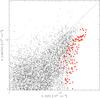 |
Fig. A.1 Relationship between emission-derived (N(LABOCA)) and extinction-derived (N(NIR)) column densities. The red symbols show the data in the area of the most massive fragment in the cloud (#5). The dashed line shows the one-to-one relationship. |
Appendix B: Definition of the Center filament crest
To measure the radial profile of the Center filament, we defined its approximate crest with lines connecting nine points. The coordinates of these points are given in Table B.1. This crest was sampled with 20 equally-spaced cuts perpendicular to it.
Points defining the crest of the Center filament.
All Tables
All Figures
|
Fig. 1 Left: dust extinction map of the Chamaeleon-Musca region, based on 2MASS data (Kainulainen et al. 2009). Right: zoom-in to the Musca cloud, showing the instrument footprints of the observations employed in this work: NEWFIRM/NIR data (red rectangles), LABOCA/870 μm continuum emission (blue dashed lines, approximate coverage), SHeFI/C18O line emission (green crosses, from Hacar et al. 2016). |
| In the text | |
|
Fig. 2 Column density map of Musca (color scale), derived using NIR dust extinction mapping and data from NEWFIRM and 2MASS. The spatial resolution of the map is FWHM = 45″ and the sensitivity σ(NH) ≈ 0.4 × 1021 cm-2. The white boxes indicate three regions, which are shown in blowups in Fig. 3. The contours show the 870 μm continuum emission contours, observed with the APEX/LABOCA instrument and smoothed down to the resolution of the extinction data. The contours are drawn at the intervals of 0.03 mJy/beam, which is the 3σ rms noise of the smoothed data. |
| In the text | |
|
Fig. 3 Blowups from the NIR-derived column density map of the Musca cloud (Fig. 2). The contours start at NH = 1.5 × 1021 cm-2 and the step is 1.5 × 1021 cm-2. The lowest contour is drawn with a dotted line. The dashed lines in the Center region indicate the 1.6 pc velocity-coherent filament whose radial structure is modeled in Sect. 3.2. The numbered signs refer to the fragments identified within the cloud (see Sect. 3.1). |
| In the text | |
|
Fig. 4 Frequency distribution of column density values along the approximate crest of the Musca cloud for South (red), Center (black), and North (blue) regions. The dashed lines indicate the mean column densities. The relative standard deviation of the column density values in each region is shown in the panel. |
| In the text | |
|
Fig. 5 Mean radial column density profiles along the Center filament of the Musca cloud. The left and right panels show the mean profile on the west and east sides of the filament axis, respectively. The blue line shows the fit of Plummer-like profile, and red line shows the fit of a pressure-confined hydrostatic cylinder. The colored arrows indicate the radial ranges used in fitting the profiles. The error bars show the standard deviation of 20 individual profiles from which the mean profile is constructed. The vertical dashed line shows the FWHM size of the extinction mapping beam. |
| In the text | |
|
Fig. 6 Mean radial column density profiles along the Center filament. The red line shows the fit of a pressure-confined equilibrium model (Fischera & Martin 2012a), embedded inside a cylindric envelope. The black dashed line shows the column density profile of the filament without the surrounding envelope. The dashed vertical line shows the FWHM size of extinction mapping beam. |
| In the text | |
|
Fig. 7 Column density and velocity structure of Musca, measured approximately along the crest of the cloud (see Fig. 1). The top panel shows the dust extinction from NIR data. The second panel shows the central velocities, Vlsr. The third and bottom panels show the nonthermal velocity dispersions, σNT (noncorrected) and σNT,corr (opacity-corrected), normalized by the sound speed cs. The arrows in the bottom panel indicate upper limits. The red and blue points show the data for 13CO (2–1) and C18O (2–1), respectively. The locations of the fragments, which are closer than 100 arcsec of the cloud crest, are indicated with thin dashed lines. The thick dashed vertical lines separate the South, Center, and North regions from each other. The thick dashed horizontal line indicates the sonic velocity dispersion, and the dotted horizontal line the two times is the sonic velocity dispersion. The lower right corner of the middle panel indicates with a line a velocity gradient of 3 km s-1. The figure is a reproduction from Hacar et al. (2016). |
| In the text | |
|
Fig. A.1 Relationship between emission-derived (N(LABOCA)) and extinction-derived (N(NIR)) column densities. The red symbols show the data in the area of the most massive fragment in the cloud (#5). The dashed line shows the one-to-one relationship. |
| In the text | |
Current usage metrics show cumulative count of Article Views (full-text article views including HTML views, PDF and ePub downloads, according to the available data) and Abstracts Views on Vision4Press platform.
Data correspond to usage on the plateform after 2015. The current usage metrics is available 48-96 hours after online publication and is updated daily on week days.
Initial download of the metrics may take a while.