| Issue |
A&A
Volume 586, February 2016
|
|
|---|---|---|
| Article Number | A131 | |
| Number of page(s) | 19 | |
| Section | Planets and planetary systems | |
| DOI | https://doi.org/10.1051/0004-6361/201425369 | |
| Published online | 09 February 2016 | |
Modelling the photosphere of active stars for planet detection and characterization
1 Institut de Ciències de l’Espai (CSIC-IEEC), Campus UAB, Carrer de Can Magrans s/n, 08193 Cerdanyola del Vallès, Spain
e-mail: This email address is being protected from spambots. You need JavaScript enabled to view it.
; This email address is being protected from spambots. You need JavaScript enabled to view it.
; This email address is being protected from spambots. You need JavaScript enabled to view it.
; This email address is being protected from spambots. You need JavaScript enabled to view it.
2 Dept. d’Astronomia i Meteorologia, Institut de Ciències del Cosmos (ICC), Universitat de Barcelona (IEEC-UB), Martí Franquès 1, 08028 Barcelona, Spain
e-mail: This email address is being protected from spambots. You need JavaScript enabled to view it.
3 LESIA-Observatoire de Paris, CNRS, UPMC Univ. Paris 06, Université Paris-Diderot, 5 place Jules Janssen, 92195 Meudon Cedex, France
e-mail: This email address is being protected from spambots. You need JavaScript enabled to view it.
4 Reial Acadèmia de Ciències i Arts de Barcelona (RACAB), 08002 Barcelona, Spain
Received: 19 November 2014
Accepted: 18 November 2015
Abstract
Context. Stellar activity patterns are responsible for jitter effects that are observed at different timescales and amplitudes in the measurements obtained from photometric and spectroscopic time series observations. These effects are currently in the focus of many exoplanet search projects, since the lack of a well-defined characterization and correction strategy hampers the detection of the signals associated with small exoplanets.
Aims. Accurate simulations of the stellar photosphere based on the most recent available models for main-sequence stars can provide synthetic photometric and spectroscopic time series data. These may help to investigate the relation between activity jitter and stellar parameters when considering different active region patterns. Moreover, jitters can be analysed at different wavelength scales (defined by the passbands of given instruments or space missions) to design strategies to remove or minimize them.
Methods. We present the StarSim tool, which is based on a model for a spotted rotating photosphere built from the integration of the spectral contribution of a fine grid of surface elements. The model includes all significant effects affecting the flux intensities and the wavelength of spectral features produced by active regions and planets. The resulting synthetic time series data generated with this simulator were used to characterize the effects of activity jitter in extrasolar planet measurements from photometric and spectroscopic observations.
Results. Several cases of synthetic data series for Sun-like stars are presented to illustrate the capabilities of the methodology. A specific application for characterizing and modelling the spectral signature of active regions is considered, showing that the chromatic effects of faculae are dominant for low-temperature contrasts of spots. Synthetic multi-band photometry and radial velocity time series are modelled for HD 189733 by adopting the known system parameters and fitting for the map of active regions with StarSim. Our algorithm reproduces both the photometry and the radial velocity (RV) curves to good precision, generally better than the studies published to date. We evaluate the RV signature of the activity in HD 189733 by exploring a grid of solutions from the photometry. We find that the use of RV data in the inverse problem could break degeneracies and allow for a better determination of some stellar and activity parameters, for example, the configuration of active regions, the temperature contrast of spots, and the amount of faculae. In addition, the effects of spots are studied for a set of simulated transit photometry, showing that these can introduce variations in Rp/R∗ measurements with a spectral signature and amplitude that are very similar to the signal of an atmosphere dominated by dust.
Key words: starspots / stars: rotation / stars: activity
© ESO, 2016
1. Introduction
Stellar activity in late-type main-sequence stars induces photometric modulations and apparent radial velocity (thereafter RV) variations that may hamper the detection of Earth-like planets (Lagrange et al. 2010; Meunier et al. 2010a) and the measurement of their transit parameters (Barros et al. 2013), mass, and atmospheric properties. A number of recent studies have been focused on trying to separate the weak exoplanetary signals and the variations in the stellar signal both on light and RV curves (Dumusque 2014; Haywood et al. 2014; Robertson & Mahadevan 2014). However, we still lack detailed understanding of these stellar variations from the astrophysical point of view.
Late-type stars (i.e., late-F, G, K, and M spectral types) are known to be variable to some extent as a result of activity effects. These effects are seen in the stellar photosphere in the form of spots and faculae, but we lack an accurate model of their signature on data of photometric and spectroscopic time series. The signal of these activity patterns is modulated by the stellar rotation period. However, other phenomena also exist that may induce periodic signals in photometric and RV data. Pulsations, granulation, long-term evolution of active regions, and magnetic cycles may limit the capabilities of some planet searches. These effects need to be subtracted or accounted for in the design of survey strategies (Dumusque et al. 2011b,a; Moulds et al. 2013).
Significant improvement in our knowledge of activity effects on starlight will be crucial to fully exploit present and future planet search spectrographs (HARPS, HARPS-N, CARMENES, ESPRESSO, HIRES, APF, and SPIRou) and transit observations from space (CHEOPS, PLATO, and JWST). The most recent and comprehensive information on stellar variability comes from studies of the Kepler mission, which are based on the observation and analysis of ~150 000 stars taken from the first Kepler data release. Ciardi et al. (2011) have found that 80% of M dwarfs have a light dispersion lower than 500 ppm over a period of 12 h, while G dwarfs are the most stable group down to 40 ppm. McQuillan et al. (2012) investigated the variability properties of main-sequence stars in the Kepler data, finding that the typical amplitude and timescale increase towards later spectral types, which could be related to an increase in the characteristic size and lifetime of active regions. Kepler operates in the visible (430 to 890 nm), where stellar photometric variability is at least a factor of 2 higher than in the near- and thermal-IR (the “sweet spot” for the characterization of exoplanet atmospheres), which is due to the increasing contrast between spots and the stellar photosphere with decreasing wavelength. Timescales for stellar activity are generally different from those associated with single-transit observations (a few hours), and therefore this spectral variability can be removed. As a case in point, photometric modulations in the host of CoRoT-7 b are of the order of 2% (Lanza et al. 2010) and yet a transit with a depth of 0.03% was identified (Léger et al. 2009). Analyses of observations from Kepler have yielded comparable results.
The impact of stellar activity effects is very different in the case of primary (transit) and occultation observations. Alterations in the spot distribution across the stellar surface can modify the transit depth because of possible spot crossing events and because the ratio of photosphere and spotted areas on the face of the star changes (Oshagh et al. 2013b; Daassou et al. 2014). This can give rise to spurious planetary radius variations when multiple transit observations are considered. Correcting for this effect requires the use of very quiet stars or precise modelling of the stellar surface using external constraints (McCullough et al. 2014; Oshagh et al. 2013a, 2014). The situation is much simpler for occultations, where the planetary emission follows directly from the transit depth measurement. In this case, only activity-induced variations on the timescale of the duration of the occultation need to be corrected for to ensure that the proper stellar flux baseline is used. In the particular case of exoplanet characterization space missions, photometric monitoring in the visible will help to correct for activity effects in the near- and thermal-IR, where the planet signal is higher.
The effects of stellar activity on time series data have also been the subject of several recent studies using different methods for modelling observations of spotted stars (Lanza et al. 2003, 2010; Desort et al. 2007; Aigrain et al. 2012; Meunier et al. 2010a; Kipping 2012). Examples are the SOAP (Boisse et al. 2012) and SOAP 2.0 (Dumusque et al. 2014) codes, which implement surface integration techniques to reproduce the cross-correlation function (CCF) of an active star by using a Gaussian function or real observed solar CCFs. These include the effects of Doppler shifts and convective blueshift inhibition produced by spots and faculae, as well as the limb-brightening effect of faculae and a quadratic limb-darkening law for the quiet photosphere. As discussed by Dumusque et al. (2014), it is essential to reproduce convective blueshift effects from real line-shapes to obtain accurate RV variations. However, most of the codes only consider the effect caused by the flux differential of active regions (Boisse et al. 2012; Oshagh et al. 2013a, 2014). Desort et al. (2007) used Kurucz models together with a black-body approximation to reproduce the flux effect of spots on photometry and radial velocities, but they did not model the effects of convection inhibition in active regions. Moreover, most works reproduce the spectroscopic measurements from a single spectral line or generate the CCF from a simple Gaussian model. These types of models do not preserve all the spectral information of spots and faculae and therefore do not allow for the study of RV jitter produced at different spectral ranges and the chromatic flux variations induced by activity.
In this work we present the StarSim tool, which investigates the effects of stellar activity on spectroscopic or spectrophotometric observations by simulating full spectra from the spotted photosphere of a rotating star. We use atmosphere models for low-mass stars to generate synthetic spectra for the stellar surface, including the quiet photosphere, spots, and faculae. The spectrum of the entire visible face of the star is obtained by summing the contribution of a grid of small surface elements and by considering their individual signals. Using this simulator, time series spectra can be obtained covering any time interval (e.g., the rotation period of the star or longer). By multiplying the spectra with the specific transfer function, accounting for both the atmospherical and the instrumental response, the methodology can be used to study the chromatic effects of spots and faculae on photometric modulations and spectroscopic jitters. The results are used to investigate methods that correct or mitigate the effects of activity on spectrophotometric time series data. Some of these methods are presented and discussed for HD 189733 in Sect. 5. Our results allow us to evaluate the effects of activity patterns on the stellar flux and hence define the best strategies to optimize exoplanet searches and measurement experiments.
This paper is the first of a series presenting several activity-simulating and modelling applications of StarSim to improve our capabilities for planet detection and characterization.
2. Simulation of the photosphere of active stars
2.1. Models
2.1.1. Phoenix synthetic spectra
We chose from among the most recent model atmosphere grids the spectra from the BT-Settl database (Allard et al. 2013), which are generated with the Phoenix code. They were used to reproduce the spectral signal for the different elements in the photosphere (quiet photosphere, spots, and faculae) by considering different temperatures for the synthetic spectra. Models include revised solar oxygen abundances (Caffau et al. 2011) and a cloud formation recipe that can also reproduce the photometric and spectroscopic properties for very low mass stars. In our simulations, local thermal equilibrium (LTE) models are used for both the quiet photosphere and active regions (spots and faculae). Non-LTE (NLTE) models from Fontenla et al. (2009) will be considered in future versions of the code to model faculae because they have been shown to better reproduce the spectral irradiance of activity features throughout the magnetic cycle in the case of the Sun (Fontenla et al. 2011). Synthetic spectra from BT-Settl models are available for 2600 K <Teff< 70 000 K, +3.5 ≤ log g ≤ + 5.0, and several values of alpha enhancement and metallicity. An example for a solar-type star is shown in Fig. 1.
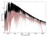 |
Fig. 1 Synthetic spectrum of a solar-like star for Teff = 5770 K and log g = 4.5 (black) generated with BT-Settl models, compared to a synthetic spectrum with a Teff value 310 K lower (brown), which could be representative of a spot. In red we plot the transmission function of the Kepler passband. |
These models include the effects of convection as described by the mixing length theory of turbulent transport (Vitense 1953) characterized by the mixing length parameter α as discussed by Ludwig et al. (1999) using 3D radiative models. Convection has a significant impact on line profiles, which are modified when active regions cross the stellar surface, and hence it is responsible for a significant part of the jitter observed in RV measurements (Meunier et al. 2010a).
A BT-Settl database of spectra is currently available for resolutions defined by a sampling ≥0.05 Å, which is not enough to study line profiles and obtain accurate RV measurements. To perform simulations for RV jitter studies and line profiles, high-resolution spectra presented by Husser et al. (2013) were used instead. The library is also based on the Phoenix code, and the synthetic spectra cover the wavelength range from 500 to 5500 nm with resolutions of R = 500 000 in the optical and near-IR, R = 100 000 in the IR, and Δλ = 0.1Å in the UV. The parameter space covers 2300 K ≤ Teff ≤ 12 000 K, 0.0 ≤ log g ≤ +6.0, −4.0 ≤ [Fe/H]≤ +1.0, and 0.2 ≤ [α/Fe] ≤ + 1.2.
2.1.2. Solar spectra
In addition to synthetic spectra from model atmospheres, observed high-resolution spectra of the Sun were used to test the results obtained with the Phoenix models. The spectra were obtained from a photospheric region and a spot with the one-meter Fourier Transform Spectrometer of the National Solar Observatory located at Kitt Peak; they have a resolution of R ~ 106 covering wavelengths from 390 nm to 665 nm. Figure 2 shows a comparison between the solar observed spectra and synthetic Phoenix spectra from Husser et al. (2013) for a Sun-like star for the quiet photosphere and a spot region. The temperature of the photospheric region was fixed to Teff = 5770 K for the synthetic spectrum, which agrees with most of the features in the observed data. In the case of the spot spectrum, Teff was varied from 4500 to 5500 K and the best agreement was found for 5460 K (temperature contrast ΔTspot = 310 K) when considering the whole wavelength range. This was done by minimizing the root mean square (rms) of the different models divided by the spectrum of the spot. The result is consistent with the measurements made by Eker et al. (2003), who determined ΔTspot ≃ 300 K for the combination of umbra and penumbra by analysing multi-channel fluxes of an equatorial passage of a sunspot.
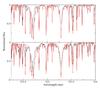 |
Fig. 2 Top: comparison between an observed high-resolution spectrum for the solar photosphere (black) and a Phoenix synthetic spectrum (red) from Husser et al. (2013) using Teff = 5770 K, log g = 4.5 and solar abundances. Bottom: same for the observed spectrum of a spot region (black), now compared with a Phoenix synthetic spectrum of Teff = 5460 K. |
2.2. Data simulation
2.2.1. Model and stellar parameters
The stellar photosphere was divided into a grid of surface elements whose physical and geometrical properties are described individually. The space resolution of the grid is an input parameter of the program, and 1° × 1° size elements were found to be adequate to correctly reproduce most active region configurations and transiting planet effects down to ~ 10-6 photometric precision. A complete list of the input parameters of the program is presented in Table 1. The table also shows the typical values considered for each parameter, based on the grid coverage of the models and on some physical constraints that are discussed below.
The StarSim tool is able to reproduce any possible distribution of active regions that can be defined with the adopted surface grid. Active regions with complex geometric properties can be defined by adding the contribution of small circular regions. The total number of active regions, as well as their surface and time distributions, can be provided as an input by the user or be randomly generated by the program following different statistics defined in the input parameters. The number of regions at a given time depends on a flat distribution between a specified minimum, Nrmin, and a maximum, Nrmax. The sizes of the spots follow a Gaussian distribution, defined by a mean area  and a standard deviation σ(ASn), in units of the total stellar surface. Therefore, the mean filling factor (
 ) over time in the whole stellar surface is determined by the mean number of spots,
  and their mean area by
  (1)We note that this filling factor only varies due to active region evolution and is different from the projected filling factor, which also accounts for the geometric projection of spots that is due to stellar inclination and rotation modulation.
Input parameters.
Although the geometric description of the spots is free (only defined by the properties of the underlying stellar grid), tests were carried out by modelling each active region n as a circular spot of radius RSn surrounded by a corona associated with a facular region that has an external radius  (see Fig. 3), where Q is the ratio between the area of the surrounding faculae and the area of the spot, which is assumed to be the same for all the active regions on the star. Our model does not distinguish between spot umbra and penumbra, but adopts a mean spot contrast at an intermediate temperature, similar to the prescription used by previous approaches (Chapman 1987; Unruh et al. 1999). The model of circular spots surrounded by a corona of faculae has been shown to successfully reproduce spot maps for the Sun (Lanza et al. 2003) and for several low-mass stars with high-precision light curves (Lanza et al. 2009, 2010; Silva-Valio et al. 2010). Solar observations have shown that the contrast and size of faculae change systematically (Chapman 1987), with the value Q decreasing for larger active regions that are more frequent around the maximum of activity (Chapman et al. 2011). Foukal (1998) showed that the relationship between the area of the faculae and the area of the spots is not linear and can vary from Q ~ 2 to Q ~ 10 depending on the size and lifetime of the active regions. In our case, we chose values from Q ~ 3 to Q ~ 8, representing medium- and small-sized spots for the simulations of Sun-like star data. Several studies on the modelling of high-precision light curves conclude that lower values of Q or even Q = 0 (i.e., no faculae) provide the best description of the data for K and early-M dwarfs (Gondoin 2008; Lanza et al. 2010, 2011b). In our work we investigate and discuss the appropriate presence of faculae to be included in the simulations of each particular case.
The geometric distribution of the active regions is not constrained in the StarSim tool, which means that this can be either user defined or generated randomly. In the second case, the longitudes of the active regions are equally distributed over the stellar surface, while the latitudes are distributed in two belts defined by Gaussian functions centred at  . This configuration can be used to simulate butterfly diagram evolution patterns, which are well known for the Sun (Jiang et al. 2011; Vecchio et al. 2012) and several active dwarfs (Katsova et al. 2003; Berdyugina & Henry 2007; Livshits et al. 2003), together with other long-term variations (Pulkkinen et al. 1999). Spot latitudes have also been measured for several stars from observations of spot crossing events (Sanchis-Ojeda & Winn 2011).
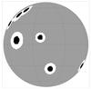 |
Fig. 3 Projected map for an arbitrary distribution of active regions with Q = 3.0. The quiet photosphere is represented in grey, and each active region is modelled as a cold spot (black) and a hotter surrounding area associated with faculae (white). |
Active region evolution can also be modelled with StarSim. This is done by considering a linear increase of the spot sizes with time, followed by a time interval of constant size and a final decay. In the case of selecting a random distribution of the parameters of the active regions, the total typical lifetime of active regions,  , its standard deviation, σ(Ln), and the growth or decay rate, ard, are also specified when configuring the simulation. Spots are known to live for weeks on main-sequence stars and for months in the case of locked binary systems (Hussain 2002; Strassmeier et al. 1994a,b). However, polar star spots have been observed to last for years (Olah & Pettersen 1991). Measurements of the decay rate of sunspots have shown that this decay follows a parabolic area decay law (Petrovay & van Driel-Gesztelyi 1997; Petrovay et al. 1999), although previous studies assumed both linear and non-linear laws (Martinez Pillet et al. 1993). Doppler imaging observations of isolated starspots over time are not yet available in high resolution for other stars. We considered a parabolic law for the decay and the emergence of the active regions, and the evolution rate was set to solar values except for stars where the surface map has been modelled for a long enough time span to estimate spot lifetimes and observe variations in size.
In the current implementation, our simulator is not intended to model each active region as a group of small spots, but to consider it as a single circular spot. We assume that this approach, by considering the appropriate size and evolution of the active regions, generates mostly the same effects on the simulated photometric and spectroscopic data as using a more complicated group-pattern configuration. We adjusted the number and size of active regions so that they agree with the results from the literature, which assumed a two-temperature structure (Henry et al. 1995; Rodonò et al. 2000; Padmakar & Pandey 1999). Solanki & Unruh (2004) discussed the distribution of spot sizes for some Sun-like stars observed with the Doppler imaging technique. Although it is suggested that sizes could follow a lognormal distribution as on the Sun, we did not adopt this distribution because the smaller spots would not cause a significant effect in our simulations compared to large spots, especially for the most active stars where large spots dominate (Solanki & Unruh 2004; Jackson & Jeffries 2013; Strassmeier 2009).
Spot temperatures have only been determined in a few cases, and the inhomogeneity of the results caused by the diversity of techniques make this a still-unconstrained parameter. Most of the current measurements made in main-sequence stars come from Doppler imaging (Marsden et al. 2005; Strassmeier & Rice 1998) or multi-band light-curve modelling (Petrov et al. 1994; O’Neal et al. 2004). The first are limited to young fast-rotating active stars that can present a different kind of activity pattern (Mullan & MacDonald 2001), and it is not clear that these results can be extrapolated to the active regions in Sun-like stars. Berdyugina (2005) showed that on average, the spot temperature contrast ΔTspot depends on the spectral type and is higher for hotter stars. However, spot temperatures appear to be uncorrelated to sizes (Bouvier & Bertout 1989; Strassmeier 1992) or activity cycles (Stix 2002; Albregtsen & Maltby 1981; Penn & MacDonald 2007) in the case of the Sun. In our simulations we assumed the same ΔTspot for all the active regions, which is estimated from a low-order polynomial fit to the data in Berdyugina (2005),  (2)This is consistent with the temperature measurements of the darkest regions of the spot in the case of the Sun (Eker et al. 2003). When possible, we used more accurate determinations of the whole spot region properties based on their spectral signature (see Sect. 3; also Pont et al. 2008, 2013; Sing et al. 2011).
As explained in Sect. 2.1.1, Phoenix models are used to reproduce the spectral signature of faculae in our approach. Faculae are known to be mainly a magnetic phenomenon affecting the intensity of the spectral lines; faculae are best reproduced by NLTE simulations (Carlsson & Stein 1992). The lack of high-resolution models for faculae in the spectral range of our interest prevents us from including them in high-resolution spectra simulations and restricts them to the simulations of broad-band photometric variations (see Sect. 2.2.2). A positive temperature contrast between the faculae and the photosphere ΔTfac ≃ 30−50 K is assumed, as reported by Badalyan & Prudkovskii (1973) from observations of the CO line in faculae and by Livshits & Polonskii (1968) from a more theoretical point of view. Solanki (1993) discussed this extensively and provided references on the weakening of lines in faculae and the ΔTfac that is required to best reproduce the continuum brightness.
A transiting planet can also be introduced in the simulations to investigate activity effects on photometric and radial velocity observations during transits. The planet is modelled as a circular black disk and is described in the same way as a spot with zero flux, but assuming a circular projection on the stellar disk. No planetary atmosphere is considered in the current implementation and so the radius of the planet does not depend on wavelength. The photometric signal for the primary transit is generated from the planet size, the ephemeris, and the orbit orientation (inclination and spin-orbit angles), which are specified as input parameters. The orbital semi-major axis is computed from the orbital period, Pplanet, and the stellar mass, M∗, using Kepler’s third law by assuming M∗ ≫ mplanet. Eccentricity is considered to be zero for all cases in the current model.
Together with the physical parameters of the star-planet system, the spectral range for the output data, the time span of the simulations and the cadence of the data series can be selected. The program generates the resulting time-series spectra and also creates a light curve by multiplying each generated spectrum by a filter passband specified from a database. If preferred, a filter with a rectangular transfer function can be defined and used to study the photometric signal at any desired wavelength range. Finally, the integration time, the telescope collecting area, the efficiency of the instrument, and the target star magnitude are needed to apply photon noise statistics to the resulting fluxes.
2.2.2. Simulating photometric time series
To build the spectrum of the spotted stellar surface, three initial synthetic spectra generated from models with different temperatures are computed for the quiet photosphere, spots, and faculae. The program reads the physical parameters for the three photospheric features of the modelled star and interpolates in Teff within the corresponding model grids to generate the three synthetic spectra: fp(λ),fs(λ), and ff(λ). The rest of the stellar parameters (log g, metallicity, etc.) are not significantly variable over the stellar surface, and specifically not for active regions. Therefore, their precision is not critical for the purpose of our simulations, and the nearest grid values are considered instead of interpolations.
Kurucz (ATLAS9) spectra are computed for the specified parameters that reproduce the photosphere and the spots. These models provide information on the intensity profile of the star, which can be used to compute the limb-darkening factors, I(λ,μ) /I(λ,0). With our approach, this factor is computed separately for every surface element and wavelength. This is done by interpolating within the grid of intensities provided by the Kurucz models. Then, the spectrum of the undarkened surface element (fp(λ) for the quiet photosphere or fs(λ) for the spots) is multiplied by the corresponding limb-darkening factor, Ip(λ,μ) /Ip(λ,0) or Is(λ,μ) /Is(λ,0) (see Eqs. (4), (10), and (14)). In the case of faculae, a different approach is considered because it is known that these areas are brightened near the limb (Frazier & Stenflo 1978; Berger et al. 2007). A limb-brightening law is considered in this case, as presented in Eq. (13).
The code produces time-series data considering the initial and final times and the cadence of the time series specified in the input parameters. For each time step, the evolutionary stage (current size) and the projected position of each active region are computed. This last parameter is obtained from the specified rotation period, P0, and the differential rotation of the star, which is modelled as described by Beck (2000):  (3)where Ω0 is the equatorial rate, Ω⊙ A = 1.698° day-1 and Ω⊙ B = 2.346° day-1 are the coefficients that describe the differential rotation for the Sun (Snodgrass & Ulrich 1990), krot is a factor that sets the differential rotation rate for the star and is specified in the input parameters (the value for the Sun would be krot = 1), and θ is the colatitude.
In a first step, the spectrum for the quiet photosphere is obtained from the contribution of all the surface elements, taking into account the geometry of the element, its projection towards the observer, the corresponding limb-darkening profile, and the RV shift: 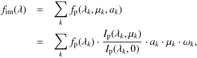 (4)where k is the surface element and μk is the cosine of its projection angle given by
  (5)where θk and φk are the colatitude and longitude coordinates, respectively, and i∗ is the stellar axis inclination.
The factor ωk accounts for the visibility of the surface element and is given by 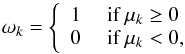 (6)and ak is the area of the surface element, which can be computed from the spatial resolution of the grid (Δα) by
  (7)Finally, λk are the wavelengths including the Doppler shift for the corresponding surface element,
  (8)with
 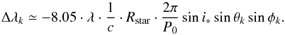 (9)These are computed from the equatorial rotation period given in the input parameters and the stellar radius calculated using its relation with log g and Teff for main-sequence stars.
The flux variations produced by the visible active regions are added to the contribution of the immaculate photosphere when computing the spectrum at each time step j. These are given by ![Mathematical equation: \begin{eqnarray} \Delta f^{\rm ar}_{j}(\lambda)& = & \sum\limits_{k} \left[\left(f_{\rm s}(\lambda_{k}) \cdot J^{kj}_{\rm s}(\lambda_{k})-f_{\rm p}(\lambda_{k}) \cdot J^{kj}_{\rm p}(\lambda_{k})\right) \cdot p^{kj}_{\rm s} \right.\nonumber \\ &&\left.+ \left(f_{\rm f}(\lambda_{k}) \cdot J^{kj}_{\rm f}-f_{\rm p}(\lambda_{k}) \cdot J^{kj}_{\rm p}(\lambda_{k})\right) \cdot p^{kj}_{\rm f}\right], \label{eqdeficit} \end{eqnarray}](/articles/aa/full_html/2016/02/aa25369-14/aa25369-14-eq101.png) (10)where the first term accounts for the flux deficit produced by the spots and the second is the overflux produced by faculae. The quantities
(10)where the first term accounts for the flux deficit produced by the spots and the second is the overflux produced by faculae. The quantities  ,
,  and
and  account for the geometric and the limb-darkening or -brightening factors for the surface element k at the time step j of the simulation, and are given by
 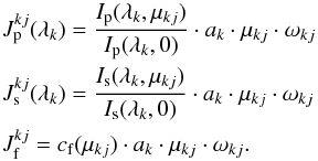 (11)The factors
  and
and  are the fractions of the surface element k covered by spot and faculae, respectively. These amounts are computed for every surface element considering their distance to the centre of all the neighbouring active regions at each observation j. The projection of the surface elements also depends on time, which is given by
 ![Mathematical equation: \begin{equation} \mu_{kj}=\sin i_{*} \sin \theta_{k} \cos \left[\phi_{k} + \Omega(\theta) \cdot (t_{j}-t_{0})\right] + \cos i_{*} \cos \theta_{k}. \label{mu} \end{equation}](/articles/aa/full_html/2016/02/aa25369-14/aa25369-14-eq108.png) (12)Finally, cf(μkj) accounts for the limb brightening of faculae, which is assumed to follow the law used by Meunier et al. (2010a):
(12)Finally, cf(μkj) accounts for the limb brightening of faculae, which is assumed to follow the law used by Meunier et al. (2010a): 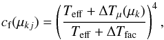 (13)where
 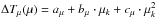 .
.
The coefficients are aμ = 250.9, bμ = −407.4 and cμ = 190.9, so that cf(μkj) ~ 1 at the centre of the disk and ~ 1.16 near the limb for a Sun-like star with ΔTfac = 30 K. This agrees with the parametrizations presented by Unruh et al. (1999). The observations show that the contribution of faculae dominate the irradiance in the case of the Sun, where active regions are ~1.2 times brighter at the limb than at the centre of the stellar disk (Ortiz et al. 2002; Ball et al. 2011; Steinegger et al. 1996).
As explained in Sect. 2.2.1, a transiting planet can be included as a dark circular spot with a constant radius over wavelength (no atmosphere) crossing the stellar disk. For each time step j, the planet position is obtained from the given ephemeris and the flux deficit is computed from the eclipsed surface elements of the star:  (14)where
  is the fraction of the surface element k covered by the planet at time step j. If an active region is partially occulted by the planet, the corresponding spot () and facula () fractions (see Eq. (10)) in the occulted surface elements are computed within the planet-covered fraction () instead.
Finally, the spectrum for the observation j is obtained by adding the contribution of the immaculate photosphere, the active regions, and the transiting planet: 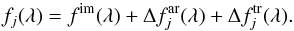 (15)When working with the low-resolution Phoenix spectra to produce a photometric time series, the resulting spectra are multiplied by the specified filter passband (see Fig. 1) to obtain the total flux and to compute the jitter produced by activity at the desired spectral range. The photometric jitter is evaluated by computing the rms of the flux over time for the whole photometric data series.
A comparison between two light curves obtained from Phoenix models and solar observed spectra for the Johnson-V-band is presented in Fig. 4. The simulation covers one rotation period of a Sun-like star with a single circular spot and no faculae. The spot is located on the equator and covers ~ 0.3% of the visible stellar surface. The temperature contrast of the spot, ΔTspot, was fitted considering 10 K steps in the Phoenix spectrum of the spot and minimizing the rms of the residuals between the two light curves. The best solution was found for ΔTspot = 320 K, presenting differences at the 10-5 level, which closely agrees with the contrast found by direct determination from the spectra (see Sect. 2.1.2). We conclude that the small deviations shown by the models for specific spectral lines do not have a significant impact at the required photometric level when considering broad spectral bands.
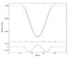 |
Fig. 4 Top panel: comparison between two light curves obtained for a star with Teff = 5777 K, log g = 4.5 and ΔTspot = 320 K from Phoenix BT-Settl models (red) and solar observed spectra (black), by introducing an equatorial spot covering ~ 0.3% of the visible stellar surface. Bottom panel: difference between the two light curves. |
The position of the photocenter on the stellar disk is also computed for each time step j of the simulations. This is implemented for a further investigation of the astrometric jitter caused by the presence of active regions or transiting planets. The astrometric shifts depend on wavelength and are computed separately for the equatorial axis (X) and the spin projected axis of the star (Y) by ![Mathematical equation: \begin{eqnarray} \Delta X^{j}(\lambda)& = &\sum\limits_{k} \left\{f_{\rm p}(\lambda_{k}) \cdot J^{kj}_{\rm p}(\lambda_{k})\cdot x_{kj}\right. \nonumber\\ &&\quad + \left[f_{\rm s}(\lambda_{k}) \cdot J^{kj}_{\rm s}(\lambda_{k})-f_{\rm p}(\lambda_{k})\cdot J^{kj}_{\rm p}(\lambda_{k})\right] \cdot p^{kj}_{\rm s} \cdot x_{kj} \nonumber\\ &&\quad + \left[f_{\rm f}(\lambda_{k})\cdot J^{kj}_{\rm f}-f_{\rm p}(\lambda_{k})\cdot J^{kj}_{\rm p}(\lambda_{k})\right]\cdot p^{kj}_{\rm f}\cdot x_{kj} \nonumber \\ &&\quad\left. + f_{\rm p}(\lambda_{k}) \cdot J^{kj}_{\rm p}(\lambda_{k}) \cdot p^{kj}_{\rm tr} \cdot x_{kj}\right\} \label{astroshX} \end{eqnarray}](/articles/aa/full_html/2016/02/aa25369-14/aa25369-14-eq128.png) (16)and
(16)and ![Mathematical equation: \begin{eqnarray} \Delta Y^{j}(\lambda) &=& \sum\limits_{k}\left \{f_{\rm p}(\lambda_{k}) \cdot J^{kj}_{\rm p}(\lambda_{k})\cdot y_{kj} \right.\nonumber\\ &&\quad + \left[f_{\rm s}(\lambda_{k}) \cdot J^{kj}_{\rm s}(\lambda_{k})-f_{\rm p}(\lambda_{k})\cdot J^{kj}_{\rm p}(\lambda_{k})\right] \cdot p^{kj}_{\rm s} \cdot y_{kj} \nonumber\\ &&\quad + \left[f_{\rm f}(\lambda_{k})\cdot J^{kj}_{\rm f}-f_{\rm p}(\lambda_{k})\cdot J^{kj}_{\rm p}(\lambda_{k})\right]\cdot p^{kj}_{\rm f}\cdot y_{kj} \nonumber \\ &&\quad \left.+ f_{\rm p}(\lambda_{k}) \cdot J^{kj}_{\rm p}(\lambda_{k}) \cdot p^{kj}_{\rm tr} \cdot y_{kj}\right\}, \label{astroshY} \end{eqnarray}](/articles/aa/full_html/2016/02/aa25369-14/aa25369-14-eq129.png) (17)where the quantities
(17)where the quantities  ,
,  and
and  are given by Eq. (11) and xkj and ykj denote the position of the surface element k projected on the X and Y axes, respectively, at the time step j of the simulation. The rest of the variables are defined in Eqs. (4) to (14).
The first term in Eqs. (16) and (17) provides the position of the photocenter for an immaculate photosphere, whereas the second, third, and fourth terms add the contribution of spots, faculae, and planet to the astrometric shifts. As in Eq. (14), the corresponding flux contribution is computed within and subtracted from or , when the planet occults a surface element k that contains a spot or a facula, respectively.
ΔXj(λ)and ΔYj(λ) vectors are finally multiplied by a given instrumental response function or a filter passband to produce astrometry displacement curves. Two simple cases are presented in Fig. 5 for a Sun-like and a K0-type star observed at i = 90°. A single circular active region was considered, consisting of a spot of size ASn = 1.6 × 10⁻³ relative to the stellar surface and a surrounding facular area with Q = 3.0, located on the equator of the star (θ = 90°). The temperature contrast of the spot was set to ΔTspot = 310 K for the Sun-like star and ΔTspot = 250 K for the K0 star (see Sect. 2.2.1 and Berdyugina 2005). The photometric signature can be seen in the top panel, which is dominated by faculae when the active region appears at the edges of the stellar disk (phases ~ 0.3 and ~ 0.7) as an effect of limb brightening, while the dark spot produces a decrease of ~ 0.001 in relative flux units at the centre of the stellar disk (phase ~ 0.5). The astrometric signature (middle panel) peaks at ± 0.001R∗. This jitter would only affect astrometric measurements at the expected precision of the Gaia space mission (Lindegren et al. 2008; Eyer et al. 2013) for main-sequence stars located at 20 pc or closer. A more detailed analysis and discussion of astrometric jitter simulations will be presented in a future paper.
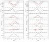 |
Fig. 5 Simulations of an active region located on the equator θ = 90° with a size of ASn = 1.6 × 10⁻³ relative to the stellar surface. The rotation period is 25 days and the inclination is 90°, yielding vsini = 2 km s-1. Left panels: simulated data for a Sun-like star (Teff = 5770 K) and ΔTspot = 310 K. Right panels: the same for a K0 star (Teff = 5000 K) and ΔTspot = 250 K. From top to bottom: photometric (in Johnson V-band), astrometric, RV, FWHM, BIS, and S index variations induced by the active region. The results with surrounding faculae (Q = 3) are shown with black solid lines and those without faculae (Q = 0) are plotted with black dashed lines. The same simulations made with SOAP 2.0 are plotted with red lines. |
2.2.3. Simulating spectroscopic data
A similar method as the one presented in Sect. 2.2.2 is implemented for the simulation of time series data to obtain activity-induced RV curves. A drawback of the method we used is the large volume of data produced when working with high-resolution spectra, which is solved by working in the velocity space, as explained below.
Three synthetic spectra (fp(λ),fs(λ) and ff(λ)) for the given wavelength range are computed for different temperatures corresponding to the quiet photosphere, spots, and faculae by interpolating from the Husser et al. (2013) Phoenix library (see Sect. 2.1.1). The values in the grid that are nearest to the specified ones are considered for the remaining parameters, as done in Sect. 2.2.2. Then, individual CCFs (Cp(v),Cs(v), and Cf(v)) are computed from the three spectra and a template mask consisting of a synthetic spectrum of a slowly rotating inactive star of the same parameters. In the current version of StarSim, the mask templates from the HARPS instrument pipeline (DRS,Cosentino et al. 2012) are used to compute the CCF contribution of the different elements (Pepe et al. 2002, 2004). These are optimized for G2, K5, and M2 type main-sequence stars and consist of a selection of delta-peak lines, whose height corresponds to the line equivalent width.
The global CCF of the projected stellar surface is computed from the contribution of the individual surface elements. First, the signature of the immaculate photosphere is obtained from  (18)where the quantity
  accounts for the intensity and geometric factors of the surface element k,
  (19)The summation covers the whole wavelength range specified for fp(λ).
The shifted velocities, vk, are computed from the contribution of the Doppler shift and the effects of convection,  (20)for l = { p,s,f }, where
  is the contribution from the Doppler shift for the surface element k (see Eq. (9)) and
  is the effect of convective blueshift, which depends on the line depth and can be characterized by studying the line bisectors, which will typically show a distinctive C-shape that is due to granulation in the photosphere (Gray 1992).
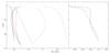 |
Fig. 6 Left panel: line bisectors computed using the full HARPS instrument range (~380−670 nm) from CIFIST 3D model spectra at μ = 1.0 (black solid line), μ = 0.79 (black dashed line), μ = 0.41 (black dot-dashed line), and μ = 0.09 (black dotted line). We also show line bisectors for observed solar spectra for a quiet-Sun region (red solid line) and a spot (red dashed line) and the bisector computed with StarSim from the integrated CCF of an unspotted photosphere of a Sun-like star (blue solid line). Right panel: zoom of the left part of the left plot showing a comparison with the bisectors of the Sun-like stars α Cen A (green solid line) and 18 Sco (orange solid line) observed with the HARPS South instrument (X. Dumusque, private communication). |
The effects of convection in the line profile are included in the Phoenix spectra from Husser et al. (2013) (see Sect. 2.1) assuming a surface element in LTE observed at μ = 1. However, this description is too simple and only valid for surface elements located at the centre of the stellar disk. Therefore, we decided to employ a more sophisticated treatment introducing the convective blueshift from CIFIST 3D models (Ludwig et al. 2009) including NLTE effects. The convection effects of the Phoenix spectra were fitted with a low-order polynomial function to the CCF computed with the full spectral range, and then subtracted. Next, we added the convective blueshift contribution computed from the 3D models. They are available for a Sun-like star and several projection angles ranging from the disk centre to the stellar limb (C. Allende Prieto, priv. comm.). We computed the CCFs and then fitted low-order polynomial functions to the line bisectors for the different available projection angles. Then, we obtained the  ,
,  and
and  for any projection angle μk from a linear interpolation of the available models. In the case of the active regions (i.e., both spot and facula zones), where convection is known to be blocked by strong magnetic fields (see Strassmeier 2009 and references therein), the solar spectra observed with high resolution described in Sect. 2.1.2 were used to compute the shift in the line bisector with respect to the photosphere. This was then scaled with μ and added to the amounts and of the surface elements where a contribution of spot or faculae was present. In this way, the contribution of active regions was redshifted ~ 0.3 km s-1 (see Fig. 6) because convection is inhibited (Dumusque et al. 2014).
Figure 6 shows four of the bisectors computed by using the full HARPS wavelength range (~380−670 nm) from CIFIST 3D model spectra and by using the solar observed spectra for a quiet-Sun region and a spot. The right panel also shows a comparison with the bisectors of 18 Sco and α Cen A, which have very similar physical properties as the Sun and were observed with HARPS at a minimum activity level (X. Dumusque, priv. comm.). They are displayed together with the simulation of the bisector of a spotless photosphere of a Sun-like star generated with StarSim. The differences are below ~10−20 m s-1 and <10 m s-1 for contrasts <0.9, so that the simulated bisectors reproduce the general behavior of the HARPS observations. The differences at the top of the bisector could be due to deviations from the real limb-darkening profile, that is, having more weight at the stellar disk centre would increase the effect of C-shaped lines. Moreover, a better modelling of convection effects on shallow lines would be needed to improve the agreement on this part of the bisector.
The vertical component of the convective velocity produces a maximum shift at the centre of the stellar disk, while the effect is barely visible near the limb where the projected velocity is zero. On the other hand, an apparent redshift of the spectral lines in comparison to the quiet photosphere is observed in spotted and facular areas as convective motions are blocked (Meunier et al. 2010b). Therefore, convection effects will introduce the strongest shift in RV measurements when a dark spot crosses the centre of the stellar disk.
The variations produced by active regions on the observed CCF at each time step j of the simulation are given by ![Mathematical equation: \begin{eqnarray} \Delta C^{\rm ar}_{j}(v) &= & \sum\limits_{k} \left\{\left[C_{\rm s}(v_{k}) \cdot H^{kj}_{\rm s}-C_{\rm p}(v_{k}) \cdot H^{kj}_{\rm p}\right] \cdot p^{kj}_{\rm s} \right. \nonumber \\ &&\left. + \left[C_{\rm f}(v_{k}) \cdot H^{kj}_{\rm f}-C_{\rm p}(v_{k}) \cdot H^{kj}_{\rm p}\right] \cdot p^{kj}_{\rm f}\right\}, \label{eqCdeficit} \end{eqnarray}](/articles/aa/full_html/2016/02/aa25369-14/aa25369-14-eq172.png) (21)where the quantities ,
(21)where the quantities ,  and
and  are computed by
 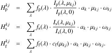 (22)The first term in Eq. (21) provides the spot contribution, while the second is the contribution for the regions with faculae.
The effect of a transiting planet is modelled as a circular dark spot. Therefore, the variations produced on the global CCF can be computed by 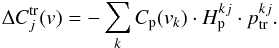 (23)As in Eqs. (14), (16), and (17), if the planet occults part of an active region, the corresponding fraction of the surface is computed within instead of the occulted or .
Finally, the total CCF simulated for the observation j is obtained by adding the contribution of the active regions (Eq. (21)) and the transiting planet (Eq. (23)) to the signature of the unspotted photosphere (Eq. (18)): 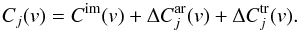 (24)The function Cj(v) is fitted with a Gaussian profile using a least-squares algorithm to obtain an accurate measurement of the peak, which is associated with the RV measurement for the time step j of the simulation. The fit is made for the data contained in a window of width ΔvCCF, specified in the input parameters, around the maximum of Cj(v). A value of 20 to 40 km s-1 for ΔvCCF has been tested to be optimal for the simulations of Sun-like stars. This needs to be adjusted according to the stellar rotation and radius, ensuring that the wings as well as parts of the continuum are inside the window of the CCF. The FWHM of the Gaussian fit is also provided as an output of the simulations because this is related to broadening mechanisms (Gray 1992). Finally, the bisector span is computed at each time step of the simulation from the difference between the mean of the 60 to 90% interval of the bisector of the CCF in Eq. (24) and the 10 to 40% interval. This definition accounts for the inverse slope of the bisector (BIS), as introduced by Queloz et al. (2001), and it is the value most commonly used in recent studies based on HARPS data (Baştürk et al. 2011; Figueira et al. 2013).
Figure 5 shows the spectroscopic measurements simulated for a single active region on a Sun-like (left) and a K0 star (right), including a comparison with simulations obtained with SOAP 2.0 for the same configurations. Inspection of the RV panel (third from the top) shows that the introduction of faculae (Q = 3) notably increases the influence of stellar surface with inhibited convective blueshift, thus producing a symmetric signal. The ~350 m s-1 mean difference between the quiet Sun and sunspot bisectors is the main parameter producing the RV variations. The effects of observed solar bisectors to account for the redshift in the active region introduce asymmetries in the FWHM and the BIS signatures. While they are of the same order, the differences with the SOAP 2.0 simulations in these measurements can be explained by a different approach when modelling the centre-to-limb variations of the bisectors for the quiet photosphere and active regions. While SOAP 2.0 uses the same CCF models across the full disk, in StarSim we use a more sophisticated and accurate approach of modelling the shape of the bisector by interpolating CIFIST 3D models of different μ angles (see Fig. 6). In addition, the ~350 m s-1 redshift of active regions is scaled with μ, accounting for the projection of the convective motion. As discussed in Appendix B of Dumusque et al. (2014), where a simple limb-shift model of spectral lines is implemented, the approach of SOAP 2.0 can produce spurious phase shifts in the spectroscopic measurements.
Figure 7 shows the radial velocity signature of a single active region on a Sun-like star. The effects of rotation (flux) and convection are displayed separately for the case of a spot without faculae (Q = 0) and with surrounding faculae (Q = 3.0). The flux effect dominates the total RV signal for spots, while active regions with faculae produce a convection-dominated signature. While convection is blocked for spots and faculae, the temperature contrast is much higher in the first, so that the effect of rotation is more important. These explanations and results can be generalized to rapid rotators, as shown by Dumusque et al. (2014).
The StarSim tool also computes the level of Ca ii H&K chromospheric emission by means of the S index (Wilson 1978; Vaughan et al. 1978; Duncan et al. 1984). The total emission of the visible surface of the star is computed from the contribution of all the surface elements, again accounting for the surface, projection, and limb-darkening factors of each element (see Eq. (22)). As before, to improve efficiency we first integrated the emission of a quiet star and then added the contribution from the active regions and, if necessary, subtracted the area occulted by transiting planets (similarly to Eqs. (18), (21), (23), and (24) for the CCF). The S emission from the active regions and from the quiet-photosphere elements were estimated from the measurements reported by Baliunas et al. (1995) and Hall et al. (2007) for the quiet Sun (Squiet ~ 0.164) and for the active Sun (Sact ~ 0.2), assuming a ~ 0.3% spot coverage and Q = 0 and Q = 3 (Balmaceda et al. 2009; Foukal 1998; Chapman et al. 2011). Simulated time-series data of the S index for a Sun-like star with a single spot are displayed in the bottom panel of Fig. 5. Considering the previous assumptions, the variability agrees with the measurements by Baliunas et al. (1995), which comprised several complete solar cycles.
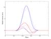 |
Fig. 7 RV shifts produced by a single spot at θ = 90° with a size of ASn = 1.6 × 10⁻³ stellar surfaces on a Sun-like star with i∗ = 90° for a simulation without (Q = 0, in red) and with faculae (Q = 3.0, in blue). The result of simulating a rotating star (Prot = 25 days) without convection is plotted with a dashed line, showing the flux effect. The simulation of a convective star without Doppler shifts is plotted with a dotted line. Both effects are included in the results plotted with a solid line. The HARPS passband is used to compute all the RVs. |
3. Simulated spectral signature of active regions
As presented in Sect. 2, StarSim allows modelling the photometric and spectroscopic variability of an active star with cool starspots and hot faculae modulated by stellar rotation. The spectral signature of active regions is defined as the dependence of the flux variability or photometric jitter introduced by active regions with the equivalent wavelength of the observations. This can only be measured from time series spectroscopy or multi-band photometry of spotted stars and provides the key for estimating spot temperatures and sizes, which remain degenerated when observations in a single photometric band are available. Pont et al. (2013) provided measurements of the temperature contrast of spots in HD 189733 (see also Pont et al. 2008; Sing et al. 2011) by computing the wavelength dependence of the amplitude of the flux increase caused by a spot occultation observed during a planetary transit, yielding ΔTspot ≥ 750 K, which is consistent with a the mean projected filling factor of 1−3% computed from the variability in the MOST photometry (Croll et al. 2007; Miller-Ricci et al. 2008; Boisse et al. 2009).
The method implemented in StarSim allows modelling the spectral signature of spots and faculae from multi-band observations of activity effects. We may adopt the flux rms as an adequate measurement of the variability in a given light curve. Simulations for a test case Sun-like star (Teff = 5777 K, log g = 4.5 and solar abundances) with a rotation period of 25 days were performed to generate time series photometry for 12 different filters, ranging from the visible to the mid-IR (Johnson UBVRI, 2MASS JHK, and Spitzer IRAC bands). The time series photometry covers 75 days with a cadence of 1 day. The stellar surface was populated with a distribution of three to eight active regions composed of spots with an average size  in units of the total stellar surface. Two different scenarios were considered regarding the presence of faculae, assuming Q = 0.0 and Q = 5.0. The temperature contrasts were initially set to ΔTspot = 350 K and ΔTfac = 30 K. The active regions were located at a mean latitude of ± 40° and evolved with a typical lifetime of 40 days.
The resulting photometric signature for each configuration was computed in the Johnson UBVRI, 2MASS JHK, and Spitzer IRAC filter passbands, thus providing the spectral signatures of the active regions computed from ~ 300 to ~ 8000 nm. These are presented in Fig. 8 together with a snapshot of the stellar surface map at the initial time of the simulations without faculae. The same active region map was used for all the simulations. In a first step, a scenario with Q = 0.0 was considered and ΔTspot = 350 K and  were assumed. The resulting spectral signature is plotted in Fig. 8. Then, we scaled the spot areas to ± 50% and searched for the ΔTspot values that preserve the flux rms in the Johnson V-band. We obtained
  K and
K and  K for the enlarged and reduced spots, respectively. The resulting spectral signatures for these two configurations of temperature contrasts and sizes of spots are also plotted in Fig. 8. While the variability differs more than 2 × 10⁻³ (relative flux units) in the ultraviolet, the signature of the spots is barely distinguishable for the three parameter configurations in the remaining spectral range. The results change significantly when faculae are included around the spots, as shown in the bottom panel of Fig. 8. We assumed Q = 5.0, which is slightly lower than the mean solar value (Chapman 1987; Lanza et al. 2003), and ΔTfac = 30 K in all cases. Then, we recomputed the spectral signature for the same three configurations previously described. In this case, the spot temperature contrasts that preserve the photometric variability in the Johnson V-band are
  K and
K and  K. The signature of active regions is dominated by the emission of bright faculae in the near- and mid-infrared, especially for the configurations with the lowest spot temperature contrasts, ΔTspot = 350 K (black line) and ΔTspot = 275 K (red line), as we see an increase in the rms after ~ 1500 nm.
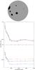 |
Fig. 8 Top panel: map of the initial distribution of active regions as used for the simulations in Sect. 3 for Q = 0.0. Middle panel: spectral signature (flux rms vs. wavelength) for three different configurations of active regions normalized to the same resulting rms in the Johnson V-band: ΔTspot = 310 K and |

These results show that determining the basic spot parameters requires spectrophotometric time series measurements at the 10-4 precision level. On the other hand, the presence and amount of faculae can be more easily measured in the red and near-IR bands, since there the photometric signature of the simulated configurations differ by ~ 10-3.
4. Modelling real data
4.1. Algorithm description
StarSim is intended to generate simulated signals from arbitrary distributions of stellar and activity parameters, as described in Sects. 2.2.2 and 2.2.3, with a better precision than other existing tools. The problem we face here is the so-called inverse problem, consisting of finding the causal factors of an observation. In this case, the aim is obtaining a dynamical spot configuration that fulfils the photometry time series. For active stars, this could be a key step for distinguishing planetary signals, especially those existing in RV data. The method used in StarSim to simulate the stellar surface is also implemented to perform the inverse problem and obtain detailed stellar surface maps that best fit the observed photometric signature produced by n − active regions. The observables are described as  (25)where yi is the measurement at time ti, fi is the model, ak are the stellar parameters, and sj is the configuration of active regions. The generation of the functions fi is described in Sect. 2.2.2 and Sect. 2.2.3 for the photometric and the spectroscopic observables, respectively.
In our case, StarSim performed a Monte Carlo simulated annealing minimization (MC-SA). This is a generic probabilistic global optimizer that allows finding a reasonably good approximation to the optimum in large configuration-space problems. Although this method has been used mainly in discrete spaces, it is also appropriate for continous problems such as the case of continuous parameters of the spot list. One of the significant advantages of this optimization technique is the proven robustness against local minima in noisy surfaces (Kirkpatrick et al. 1983), which makes it an interesting approach to optimize models involving a large number of parameters. The name of the algorithm – and its associated nomenclature – comes from the term “annealing” in metallurgy, a technique involving a scheduled cooling of metals to modify the size of crystals and reduce their defects.
The aim of the fitting process is to find a map of active regions that minimizes the χ2, 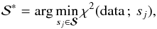 (26)where χ2 is evaluated between the model and the data,
 ![Mathematical equation: \begin{equation} \chi^2 = \sum_{i=1}^{N}\frac{[y_i - f_i]^2}{\sigma_i^2} \label{eqn:chi2_0} , \end{equation}](/articles/aa/full_html/2016/02/aa25369-14/aa25369-14-eq216.png) (27)and σi are the errors associated with de data.
(27)and σi are the errors associated with de data.
The activity map sj is defined as a set of parameters containing the coordinates, initial time, lifetime, and size of a preselected number of active regions, n,
sj= {tinit, tlife, φ (colatitude), λ (longitude), radii }, for j = 1,...,n
where sj is a specific configuration of active regions from all the possible sets,  , and
, and  is the optimal configuration.
More details on the MC-SA procedure are given in Appendix A together with the parameters used in StarSim.
4.2. Current status of StarSim
The StarSim tool is currently capable of generating simulated photometric and spectroscopic signals as described in Sects. 2.2.2 and 2.2.3. It is currently written using a combination of Fortran and C routines. The simulations ran on an Intel Core i7-3770 CPU at 3.40 GHz produced a time series of 1000 phases in 60 seconds for photometric data (see Sect. 2.2.2) of a Sun-like star in the Johnson V-band for a random distribution of four spots. For high-resolution spectroscopic data (see Sect. 2.2.3), the same simulation takes 210 s.
The algorithm for performing the inverse problem by means of a simulated annealing procedure (see Appendix A) is currently only implemented in the case of a single photometric time series. Including RV data and multiple photometric passbands would require a more sophisticated treatment of errors; this is being under consideration for a new version of the tool. At the moment, simultaneous series data for active stars are being studied with StarSim by simulating a grid of RV solutions from the best fit of the photometry. An example including a discussion of the constraints provided by the analysis on the stellar and activity parameters is presented for HD 189733 in next section.
Parameters for the system HD 189733.
5. A case example: HD 189733
5.1. System parameters
The exoplanet host HD 189733 is a bright (V = 7.67 mag) K0V-type star known to present significant rotation modulation in its light curve (Winn et al. 2007) with a period of ~ 11.9 days and to be relatively active, according to the measured chromospheric activity indices (Wright et al. 2004; Moutou et al. 2007). A hot-Jupiter planet with a short period (2.2 days) orbiting this star was first announced by Bouchy et al. (2005). Several studies have reported activity effects on the RV measurements of up to ~ 15 m s-1 (Lanza et al. 2011a; Bouchy et al. 2005) and have obtained information about the stellar surface photosphere from modelling the flux variations (Croll et al. 2007; Lanza et al. 2011a). The parameters for the HD 189733 system that are used in all the simulations in this section are presented in Table 2.
Miller-Ricci et al. (2008) studied the transit timing variations (thereafter TTVs) and the transit depth variations (thereafter TDVs) from six transit observations obtained by MOST, which monitored HD 189733 for 21 days during July – August 2006. No significant effects of spot crossing events were observed at any phase of the transits, but no detailed discussion of possible effects of non-occulted spots was presented. When a transiting planet passes in front of a star spot, the depth of the transit is shallower in a portion of the transit because the planet has crossed a dimmer region of the photosphere. For observations with a low signal-to-noise ratio that cannot resolve the event, this would affect the overall transit depth fit. Moreover, TTVs of ~1 min would be induced if a spot crossing event occurred at the ingress or egress phases of the transit. We refer to Barros et al. (2013) for an extensive discussion. On the other hand, non-occulted spots present during the transit time introduce variations of the stellar flux with chromatic dependence. Thereafter, they can produce a bias in the transit depth measurement and modify the signature of the atmosphere of the planet as studied by transmission spectroscopy. Since a spot is modelled as a cooler region on the stellar surface, its signal will be stronger in the blue, where the flux contrast increases, than in the red.
Pont et al. (2007) described some properties of the starspot groups in HD 189733 from the observation of two spot crossing events. The features observed in the transit light curves show a wavelength dependence and can be explained by the presence of cool regions with ΔTspot ~ 1000 K and a size of ~ 12 000 km to ~ 80 000 km, which corresponds to ASn of ~ 2 × 10⁻⁵ to ~ 6 × 10⁻³ in units of the total stellar surface.
Lanza et al. (2011a) obtained a more detailed map of the active region distribution by modelling MOST photometry covering 30.5 days from July 17 to August 17, 2007, and RV measurements from SOPHIE obtained for the same time span (Boisse et al. 2009). Their approach was based on reconstructing a maximum entropy map with regularization. This allows modelling the longitudinal evolution of active regions over time, but the information on the latitudes is lost, particularly when the inclination of the stellar rotation axis is close to 90°, as is the case for HD 189733. The method therefore tends to assume that the spots are located near the stellar equator and hence adopts the minimum possible size for the spots to simulate the observed variations. The results of Lanza et al. (2011a) showed that the data can be explained by the presence of between two to four active regions, yielding a photometric fit with an rms of 4.86 × 10⁻⁴ in relative flux units and a resulting RV curve that roughly agrees with the observed data (to within a few m s-1). The individual spots cover 0.2 to 0.5% of the stellar disk, and their lifetimes are comparable to or longer than the duration of the MOST observations (i.e., ~ 30 days), while the rise and decay occur over 2−5 days. In this case, the spot contrast is computed assuming a spot effective temperature of 4490 K (i.e., ΔTspot = 560 K). A different spot contrast would imply a change in the absolute spot coverage to explain the same photometric signature (Pont et al. 2007), but it would not have a significant effect on a single-band photometric time series. Fares et al. (2010) measured the equatorial and polar rotation periods and obtained 11.94 ± 0.16 days and 16.53 ± 2.43 days, respectively. This yields a relative amplitude of ΔΩ/Ω = 0.39 ± 0.18, which is very similar to that of the Sun (so we assume krot = 1). Then, the migration rates of spots measured by Lanza et al. (2011a) indicate that most of the spots are located at latitudes ranging from 40° to 80°.
5.2. Activity model
We analysed the MOST photometry dataset from 2007 (Lanza et al. 2011a). After removing the transits, the series contains 414 measurements with a mean error of 1.15 × 10⁻⁵ in relative flux units. The RV data from the SOPHIE spectrograph were obtained from July 13 to August 23, 2007, providing a data set of 33 RV measurements. The combination of these simultaneous data sets represents a great opportunity for testing the method of StarSim for obtaining a surface activity model for HD 189733.
The StarSim program with the minimization method presented in Sect. 4.1 was used to obtain a surface map for HD 189733. In a first approach, the MOST photometric dataset was modelled, no faculae were considered (see Lanza et al. 2011a), and the spot sizes were assumed to evolve with the mean solar growth or decay rate (i.e., ard ≃ 1°, Martinez Pillet et al. 1993; Petrovay et al. 1999). A map of 90 active regions with a grid resolution of 1° × 1° was fitted for their position, time of appearance, and lifetime, while the stellar parameters were fixed to those specified in Table 2. Despite considering a relatively high number of active regions, the minimization algorithm tends to concentrate the spots in groups, as expected. The number was adjusted to reduce the rms of the fit while preventing isolated small spots to appear in the modelled surface. Three maps containing 90 spots were randomly generated and used as initial conditions for three different fitting runs, and the simulated annealing procedure was performed as described in Appendix A to determine the convergence. The final rms of the residuals is 3.8 × 10⁻⁴ in relative flux units for all the solutions, which only present visible differences for the latitudes and sizes of some of the spot groups. The light curve model for the first run is shown in Fig. 9.
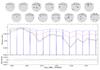 |
Fig. 9 Synthetic light curves generated for HD 189733 with the method described in Sect. 2.2.2, assuming the parameters described in Sect. 5.1 and the modelled activity map for the MOST (black line), 2 MASS J (red line), and IRAC 2 (blue line) passbands. The flux is in relative units with respect to the maximum along the light curve and shows the 14 analysed transit events. Observed data from MOST are plotted with black dots. The projected maps of the stellar surface at the mid-transit times are plotted in the upper part, including a dark grey band that indicates the region of the star occulted by the planet. |
The photometric fit that we obtain is of better quality than those published to date, and our model is able to accurately describe many of the features of the photometry. The distribution of active regions derived from the photometric fit and the parameters defined in Table 2 were adopted to synthesize the RV curve for the same time span and for the instrumental passband of SOPHIE. The result is plotted in Fig. 10 together with the SOPHIE data. The model and the observed RV variations generally agree well, except for the regions around ~HJD 2 454 309 and ~HJD 2 454 327, where a higher evolution rate for the spots is probably needed to reproduce the rapid modulations. However, we were unable to reproduce them when exploring different initial parameters for the active regions, which means that they are either caused by instrumental effects or that these variations are not caused by spots and faculae. The analyses presented by Lanza et al. (2011a) and Aigrain et al. (2012) using photometric spot models were also unable to reproduce the rapid RV variations. When excluding the three measurements between HJD 2 454 307 and 2 454 310, the rms of the residuals of our model is 5.45 m s-1, which improves the results from the previous studies (5.55 m s-1 from Lanza et al. 2011a and 6.6 m s-1 from Aigrain et al. 2012) and is close to the typical instrumental uncertainties of SOPHIE (~5 m s-1).
Another step forward in the analysis would be to include the SOPHIE RVs in the inverse problem and to perform a simultaneous fit. However, several tests indicated that the number of data points and the precision of the velocity data are too low for the fitting algorithm to work properly. As an alternative, we used the RVs to investigate the effect of several parameters that are usually adopted ad hoc or from independent criteria because of the lack of sensitivity of the light curve. The parameters are the zero point of the photometric flux (i.e., immaculate flux level), the stellar equatorial rotation period (Prot), the facula-to-spot area ratio (Q), and the temperature contrast of the active regions.
The StarSim code was used to fit the photometry with the same assumptions as described before and by exploring a grid of possible values for the four parameters in sequential and independent fashion. In this case, a model of 30 active regions was used for simplicity. The results are shown in Fig. 11. The panels on the left show the rms of the photometric fit as a function of the parameter value, while the panels on the right display the simulated RV curves compared with the observed data. As expected, all investigated parameters have very little influence on the quality of the photometric fit except for the spot temperature contrast, which shows a broad, flat minimum around ΔTspots ~ 600 K, in agreement with Lanza et al. (2011a). The variations in the photometric zero point and the rotational period of the star induce phase differences in the simulated RV curves. Figure 11 also shows that the value of Q has a very strong influence on the RV amplitude. The photometric fit, although not very significantly, favours values of Q close to 0, and this also agrees with the modest observed RV variation. The amplitude of the RV signal is also sensitive to the spot temperature contrast. The results of the simulations shown in the right panel d) indicate that ΔTspots ~ 400−500 K closely agree with the SOPHIE data, while higher values show increasing deviations.
We see notable differences in the RV simulations when we adopt different parameters, which indicates that the degeneracies might be partially broken if RV data were considered in the inverse problem. We note that the initial conditions of the distribution of active regions (positions and sizes) are randomly chosen and could also have an impact on the simulated RV curves shown in the right panels of Fig. 11. This is not a concern when the full inverse problem is considered, however, since different random realizations can be used to explore the entire parameter space. In this case, the modelling would allow for a full description of the stellar surface, including active region parameters, and thus a complete characterization of the stellar activity properties. The application of this procedure to a sample of stars would help to understand some key aspects and therefore provide means to correct RV measurements for the undesired effects of stellar activity in a self-consistent way.
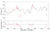 |
Fig. 10 Upper panel: RV model curve generated with StarSim for HD 189733 (black solid line) compared to the SOPHIE data (red dots). Bottom panel: residuals between the data and the model. |
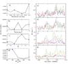 |
Fig. 11 Left panels: rms of the residuals from the fit to the MOST light curve with a model of 30 active regions vs. four stellar parameters. Right panels: simulated RV curves resulting from the models compared to the SOPHIE data (red dots). The four pairs of panels show the dependence of the rms of the light curve fits and the RV signature on a) the zero point of the photometry; b) the stellar rotation period, Prot; c) the facula-to-spot area ratio, Q; and d) the temperature contrast of the spots, ΔTspot. The colour code of the lines in the right panels corresponds to the dots in the left panels. |
5.3. Activity effects in transit photometry
Synthetic light curves for HD 189733 including planetary transits were generated using the method presented in Sect. 2.2.2 for the 12 filters used in Sect. 3 for the same time span as the MOST photometric data modelled in Sect. 5.2. This covers three complete rotation periods of the star (i.e., 14 transits of the exoplanet HD 189733b). The surface map from the photometric model obtained in Sect. 5.2, consisting of 90 spots, was considered for all the simulations. The resulting light curve has a maximum amplitude of ~ 0.012 mag in the Johnson V filter. The light curves for the 2 MASS J and the IRAC 2 passbands are plotted in Fig. 9.
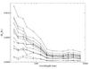 |
Fig. 12 Variations in the transit depth Rp/R∗ vs. the central wavelength of 12 different filters produced by several configurations of spots on the 14 synthetic transits of HD 189733b in the simulated light curves, relative to the transit depth in an unperturbed transit. Data affected by spot crossing events have been removed. |
For each passband, data segments of 2 × T14 (i.e., twice the total duration of the transit) around the transit mid-point were selected for analysis. The out-of-transit baselines at either side of the transit were used to fit a parabolic trend that was subsequently subtracted from the in-transit observations. The data points affected by spot crossing events were removed and not considered for analysis. Then, a Nelson & Davis (1972) model as implemented by Popper & Etzel (1981) was fitted to each individual transit using the JKTEBOP code (Southworth et al. 2004) to measure the transit depth and the mid-transit time. In a first step, precise quadratic limb-darkening coefficients were obtained for each passband by fitting a model to a transit light curve generated for an immaculate photosphere. With these limb-darkening coefficients, the full series of transits was analysed by fitting the planet radius and the zero point of the ephemeris. The rest of the parameters were fixed to those shown in Table 2.
A number of spot crossing events have been detected in HD 189733b transit observations (Miller-Ricci et al. 2008; Sing et al. 2011; Pont et al. 2013). The observed occurrence of these events combined with the assumption that the planet is crossing a typical zone of the stellar surface in terms of spot coverage, leads to an estimate of 1−2% of projected spot filling factor (Sing et al. 2011), which agrees with the results by Lanza et al. (2011a) and the spot maps used in this work. Because the active region map is poorly constrained as a result of the low signal-to-noise ratio of the MOST observations (see Lanza et al. 2011a), and especially because the latitudes of the spots are degenerated, we do not expect all the events from the MOST data to be accurately reproduced by the model for our synthetic data. For this reason, the data affected by spot crossing events were removed before fitting the transit models to study and quantify the chromatic effects of clearly visible spots.
The results of the analysis of synthetic transit data are displayed in Fig. 12, showing the chromatic dependence of the planet radius determination for each transit event. All transits present some level of influence from clearly visible spots. The measurements for Rp/R∗ are normalized at the values obtained for the transit light curve simulated on an unperturbed photosphere.
As the presence of spots in the stellar surface changes the overall transit depth measurement (i.e., the duration of the transit is much shorter than the typical changes in the projected filling factor), there are no significant differences on the measured times of mid-transit. Spots not occulted by the planet introduce a monotonic regular behaviour from the UV to mid-infrared wavelengths. Therefore, the spectral signature of the spots clearly dominates the effects introduced on the transit depth, as seen in Fig. 12. The results for the transit depth measurements are also displayed vs. the projected filling factor of spots (measured at the mid-transit times) in Fig. 13 for the 12 analysed filter passbands. The dispersion in this plot is due to the gaps introduced in the data when removing spot crossing events. For all transit simulations, the effect produced by spots is much stronger in the blue than in the mid-infrared, as a consequence of the spectral signature of the spots. The shift in the transit depth measurement introduced by clearly visible spots is scaled with the instantaneous filling factor, ranging from 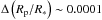 for a nearly unspotted surface (third transit, at HJD ~ 2 454 301.8 in Fig. 9) to ~ 0.001 for a projected filling factor of ~ 3% (tentth transit, near HJD ~ 2 454 319.0). This is an important information to take into account when correcting the transit depths for activity, as observations of HD 189733 show that there is significant variability in the filling factor over time. We note that to obtain the spot filling factors that affect our simulations (shown in Fig. 13), we assumed the maximum of the MOST photometry as the unit of measure for the flux to normalize the light curve (Lanza et al. 2011a). Although the evolution of the spot map we used accurately reproduces the variations, a zero point in the filling factor of spots could be present. This is still unclear from the results shown in Fig. 11, as discussed in Sect. 5.2. However, the statistics of spot crossing events during HST observations and the characteristics of the transmission spectrum in the visible (Sing et al. 2011) indicate that the projected spot filling factor is not much higher than 1−2 %.
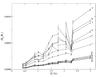 |
Fig. 13 Variations in the transit depth Rp/R∗ vs. the projected filling factor of spots at the mid-transit times for the 12 simulated passbands. |
6. Discussion and conclusions
We presented a method in the form of the StarSim tool for simulating the photosphere of rotating spotted stars. This allowed us to generate synthetic photometric and spectroscopic time series data from a set of given parameters and a library of stellar atmosphere models. The main purposes of this method are characterizing the effects produced by activity in time series observations, especially multi-band studies of exoplanetary transits, and the design of strategies for minimizing activity effects for a search and characterization of exoplanets. Several aspects need to be taken into account to discuss the reliability of the results and their interpretation.
First, we assumed LTE stellar models for the emission of the quiet photosphere and also for the spot and facula regions. This is a limitation imposed by the availability of stellar model libraries with high-resolution spectra. The synthetic spectrum shown in Fig. 2 correctly fits the observed spectrum of a spot and provides a temperature contrast that agrees with most of the values in the literature (see Sect. 2.1). However, certain lines are not well reproduced, which suggests that the spot spectrum is different from a cooler stellar photosphere. No high -resolution observed spectra are currently available for faculae, and the most recent NLTE models for the Sun are those presented by Fontenla et al. (2009). The differences in the spectrum of active regions mainly affect the existence of certain lines, but have no significant impact on the flux when considering a broad range of the spectrum. Therefore, the currently used models are suitable for characterizing activity effects in the observations for most of the photometric instrumentation. Some more considerations of the influence of the models on the different photospheric features will be discussed in a future paper that addresses strategies for correcting RV measurements in active stars. Such RV measurements are usually obtained based on the information content of the lines in the whole observed spectral range. On the other hand, optimized measurements can be made by excluding the spectral lines or ranges that are most affected by activity.
Second, given the requirements of this work, the maps of active regions currently used in our simulations are limited to a model of circular spots with a surrounding facula in the shape of a corona, instead of a more complex structure with groups of small spots. Such simple configurations of active regions have proven to adequately reproduce photometric and spectroscopic signature in active stars (Eker 1994; Lanza et al. 2003; Dumusque et al. 2014; Dumusque 2014). However, StarSim also allows modelling spots of any shape by including an unlimited number of spots of a small size on the stellar surface. Our approach is very similar to that of Lanza et al. (2003) and subsequent papers that used this type of spot maps to model the surface of active stars. In this case, the regularization of the maximum entropy algorithm provides a smooth distribution of active regions instead of a more irregular surface map populated with many small spots.
Third, several assumptions based on solar data are made in our simulations. This has to be kept in mind when using StarSim for stars that are not Sun-like. Indeed, the limb-brightening law implemented for facula regions is a model based on solar observations. The same applies to the rest of the parameters of faculae, such as the temperature contrast. The evolution rates and lifetimes of active regions have only been measured for a few stars from the various techniques that allow modelling of the stellar surface (Hussain 2002; Strassmeier et al. 1994a,b; Petrovay & van Driel-Gesztelyi 1997; Petrovay et al. 1999). While the previous assumptions affect some parameters that can be adjusted when more information from observations is available, our approach to modelling activity effects on convection is more intimately linked to solar observations in all cases. The centre-to-limb convection profile of the quiet photosphere is implemented from solar CIFIST 3D models. In addition, solar high-resolution observations are used to obtain accurate models for the bisector of active regions. Our approach to modelling convection was tested to perform at the ~1 m s-1 precision in some comparisons with Sun-like stars. Finally, the chromospheric emission data produced by our model are based on solar observations of the S index.
An example of the capabilities of the method for characterizing activity effects was presented for the case of a Sun-like star with a typical distribution of active regions. The spectral signature (flux rms vs. wavelength) of the active regions was studied in visible and IR passbands for several configurations of the stellar surface parameters. Different configurations of the temperature contrast and the typical area of the spots were found to show a very similar signature when no faculae are introduced. In the presence of faculae (Q = 5.0, ΔTfac = 30 K), the wavelength dependence is inverted in the red and near-IR wavelengths when the temperature contrast of the spots is < 300 K, which means that the contribution of faculae is dominant. In all cases, the dependence is strong in the visible and near-IR, while no signature is observed in the mid-IR. Real observations of the spectral signature for active stars in visible and near-IR filters may provide new estimates of the facula-to-spot area ratio and the spot parameters.
The effects of clearly visible spots on multiband observations of planetary transits were studied by considering the active Sun-like star HD 189733 with a transiting hot-Jupiter planet. A Monte Carlo simulated annealing minimization algorithm was implemented in StarSim and stellar surface maps were obtained by modelling the MOST photometric data for HD 189733. Several stellar parameters that are commonly assumed were explored for degeneracies by using simultaneous RV data from SOPHIE. We showed that the RV data include some additional information that can break these degeneracies, especially for the physical parameters of the active regions and the stellar surface map.
For the modelled surface map for HD 189733, we synthesised photometric light curves for 14 transits in 12 different passbands from the optical to the mid-IR, covering a variety of spot surface coverages from ~ 0.4% to ~ 3.0%, and we studied the deviations produced on the planet radius measurements. While in the first case the transit depth measurement remains unperturbed up to the 10-4 precision in Rp/R∗ for any filter passband, a strong effect is introduced when the star is moderately spotted. Moreover, the difference is wavelength dependent, being ~ 10-3 in the blue, and only ~ 5 × 10⁻⁴ in the mid-IR. Therefore, biases of the order of 10-3 can be introduced in Rp/R∗ measurements for wavelengths in the optical range if a constant spot filling factor is assumed for the clearly visible spot correction (Sing et al. 2011; Pont et al. 2013; McCullough et al. 2014) instead of considering the appropriate instantaneous spot map. Time series photometry simultaneous to the transit observation campaign would be needed to reproduce the evolution of the filling factor of spots and adequately scale the correction for each transit event. In the near future, space telescopes dedicated to exoplanetary sciences will be able to achieve precisions of ~ 10-4 on the atmosphere measurements of super-Earths (Tessenyi et al. 2012), therefore it is essential to adequately model the spectral signature of activity for these types of observations.
We conclude that the approach we presented to generate synthetic time series data accurately accounts for all the physical processes affecting spectroscopic and photometric variations produced by activity, which currently represents the main obstacle for exoplanet characterization and searches. In fact, our approach can help to model and correct for the effects of activity jitter on photometric and RV observations of extrasolar planets, especially if the system parameters are known and the surface map of the stellar host is simultaneously studied. In comparison with already existing tools to model time series data of active stars (Oshagh et al. 2013a; Boisse et al. 2012; Aigrain et al. 2012; Dumusque et al. 2014), StarSim accurately accounts for the line bisector distortions caused by convective blueshift and convection inhibition in active regions, based on recent 3D atmosphere models. Most of the cited tools assume a simple Gaussian model for the spectral lines. In StarSim we consider atmosphere models to compute the synthetic CCFs and the flux contribution of the visible surface elements of the star. This allows preserving all the spectral information of the variability produced by activity effects. Moreover, our simulations allow studying the effects of the amount of faculae as well as of spot temperature contrasts and sizes on multi-band simultaneous photometry. The methodology is currently being implemented to model fit multi-band photometric and spectroscopic RV observations simultaneously, thus obtaining detailed maps for the characterization of stellar photospheres. Several applications of the method to real observations and to the design of optimized strategies for searching and characterizing exoplanets will be presented in a series of papers in the near future. StarSim will also help to properly account for stellar activity in the detection and characterization of atmospheres in small planets.
Acknowledgments
E.H. and I.R. acknowledge support from the Spanish Ministry of Economy and Competitiveness (MINECO) and the Fondo Europeo de Desarrollo Regional (FEDER) through grants ESP2013-48391-C4-1-R and ESP2014-57495-C2-2-R. C.J. acknowledges the support by the MINECO - FEDER through grants AYA2009-14648-C02-01, AYA2010-12176-E, AYA2012-39551-C02-01 and CONSOLIDER CSD2007-00050. E. H. was supported by a JAE Pre-Doc grant (CSIC).
References
- Aigrain, S., Pont, F., & Zucker, S. 2012, MNRAS, 419, 3147 [NASA ADS] [CrossRef] [Google Scholar]
- Albregtsen, F., & Maltby, P. 1981, Sol. Phys., 71, 269 [NASA ADS] [CrossRef] [Google Scholar]
- Allard, F., Homeier, D., Freytag, B., et al. 2013, Mem. Soc. Astron. It. Suppl., 24, 128 [Google Scholar]
- Baştürk, Ö., Dall, T. H., Collet, R., Lo Curto, G., & Selam, S. O. 2011, A&A, 535, A17 [NASA ADS] [CrossRef] [EDP Sciences] [Google Scholar]
- Badalyan, O. G., & Prudkovskii, A. G. 1973, Soviet Ast., 17, 356 [NASA ADS] [Google Scholar]
- Baliunas, S. L., Donahue, R. A., Soon, W. H., et al. 1995, ApJ, 438, 269 [NASA ADS] [CrossRef] [Google Scholar]
- Ball, W. T., Unruh, Y. C., Krivova, N. A., Solanki, S., & Harder, J. W. 2011, A&A, 530, A71 [NASA ADS] [CrossRef] [EDP Sciences] [Google Scholar]
- Balmaceda, L. A., Solanki, S. K., Krivova, N. A., & Foster, S. 2009, J. Geophys. Research (Space Phys.), 114, 7104 [Google Scholar]
- Barros, S. C. C., Boué, G., Gibson, N. P., et al. 2013, MNRAS, 430, 3032 [NASA ADS] [CrossRef] [Google Scholar]
- Beck, J. G. 2000, Sol. Phys., 191, 47 [NASA ADS] [CrossRef] [Google Scholar]
- Berdyugina, S. V. 2005, Liv. Rev. Sol. Phys., 2, 8 [Google Scholar]
- Berdyugina, S. V., & Henry, G. W. 2007, ApJ, 659, L157 [NASA ADS] [CrossRef] [Google Scholar]
- Berger, T. E., Rouppe van der Voort, L., & Löfdahl, M. 2007, ApJ, 661, 1272 [NASA ADS] [CrossRef] [Google Scholar]
- Boisse, I., Moutou, C., Vidal-Madjar, A., et al. 2009, A&A, 495, 959 [NASA ADS] [CrossRef] [EDP Sciences] [Google Scholar]
- Boisse, I., Bonfils, X., & Santos, N. C. 2012, A&A, 545, A109 [NASA ADS] [CrossRef] [EDP Sciences] [Google Scholar]
- Bouchy, F., Udry, S., Mayor, M., et al. 2005, A&A, 444, L15 [NASA ADS] [CrossRef] [EDP Sciences] [Google Scholar]
- Bouvier, J., & Bertout, C. 1989, A&A, 211, 99 [NASA ADS] [Google Scholar]
- Caffau, E., Ludwig, H.-G., Steffen, M., Freytag, B., & Bonifacio, P. 2011, Sol. Phys., 268, 255 [NASA ADS] [CrossRef] [Google Scholar]
- Carlsson, M., & Stein, R. F. 1992, ApJ, 397, L59 [NASA ADS] [CrossRef] [Google Scholar]
- Chapman, G. A. 1987, ARA&A, 25, 633 [NASA ADS] [CrossRef] [Google Scholar]
- Chapman, G. A., Dobias, J. J., & Arias, T. 2011, ApJ, 728, 150 [NASA ADS] [CrossRef] [Google Scholar]
- Ciardi, D. R., von Braun, K., Bryden, G., et al. 2011, AJ, 141, 108 [NASA ADS] [CrossRef] [Google Scholar]
- Cosentino, R., Lovis, C., Pepe, F., et al. 2012, in SPIE Conf. Ser., 8446, 1 [Google Scholar]
- Croll, B., Matthews, J. M., Rowe, J. F., et al. 2007, ApJ, 671, 2129 [NASA ADS] [CrossRef] [Google Scholar]
- Daassou, A., Benkhaldoun, Z., Ait Moulay Larbi, M., & Elazhari, Y. 2014, ArXiv e-prints [arXiv:1407.1280] [Google Scholar]
- Desort, M., Lagrange, A.-M., Galland, F., Udry, S., & Mayor, M. 2007, A&A, 473, 983 [NASA ADS] [CrossRef] [EDP Sciences] [Google Scholar]
- Dumusque, X. 2014, ApJ, 796, 133 [NASA ADS] [CrossRef] [Google Scholar]
- Dumusque, X., Santos, N. C., Udry, S., Lovis, C., & Bonfils, X. 2011a, A&A, 527, A82 [NASA ADS] [CrossRef] [EDP Sciences] [Google Scholar]
- Dumusque, X., Udry, S., Lovis, C., Santos, N. C., & Monteiro, M. J. P. F. G. 2011b, A&A, 525, A140 [NASA ADS] [CrossRef] [EDP Sciences] [Google Scholar]
- Dumusque, X., Boisse, I., & Santos, N. C. 2014, ApJ, 796, 132 [NASA ADS] [CrossRef] [Google Scholar]
- Duncan, D. K., Frazer, J., Lanning, H. H., et al. 1984, PASP, 96, 707 [NASA ADS] [CrossRef] [Google Scholar]
- Eker, Z. 1994, ApJ, 420, 373 [NASA ADS] [CrossRef] [Google Scholar]
- Eker, Z., Brandt, P. N., Hanslmeier, A., Otruba, W., & Wehrli, C. 2003, A&A, 404, 1107 [NASA ADS] [CrossRef] [EDP Sciences] [Google Scholar]
- Eyer, L., Holl, B., Pourbaix, D., et al. 2013, Central European Astrophysical Bulletin, 37, 115 [NASA ADS] [Google Scholar]
- Fares, R., Donati, J.-F., Moutou, C., et al. 2010, MNRAS, 406, 409 [NASA ADS] [CrossRef] [Google Scholar]
- Figueira, P., Santos, N. C., Pepe, F., Lovis, C., & Nardetto, N. 2013, A&A, 557, A93 [NASA ADS] [CrossRef] [EDP Sciences] [Google Scholar]
- Fontenla, J. M., Curdt, W., Haberreiter, M., Harder, J., & Tian, H. 2009, ApJ, 707, 482 [NASA ADS] [CrossRef] [Google Scholar]
- Fontenla, J. M., Harder, J., Livingston, W., Snow, M., & Woods, T. 2011, J. Geophys. Res., 116, 20108 [CrossRef] [Google Scholar]
- Foukal, P. 1998, ApJ, 500, 958 [NASA ADS] [CrossRef] [Google Scholar]
- Frazier, E. N., & Stenflo, J. O. 1978, A&A, 70, 789 [NASA ADS] [Google Scholar]
- Gondoin, P. 2008, A&A, 478, 883 [NASA ADS] [CrossRef] [EDP Sciences] [Google Scholar]
- Gray, D. F. 1992, The observation and analysis of stellar photospheres (Cambridge University Press) [Google Scholar]
- Hall, J. C., Lockwood, G. W., & Skiff, B. A. 2007, AJ, 133, 862 [NASA ADS] [CrossRef] [Google Scholar]
- Haywood, R. D., Collier Cameron, A., Queloz, D., et al. 2014, MNRAS, 443, 2517 [NASA ADS] [CrossRef] [Google Scholar]
- Henry, G. W., & Winn, J. N. 2008, AJ, 135, 68 [NASA ADS] [CrossRef] [Google Scholar]
- Henry, G. W., Eaton, J. A., Hamer, J., & Hall, D. S. 1995, ApJS, 97, 513 [NASA ADS] [CrossRef] [Google Scholar]
- Hussain, G. A. J. 2002, Astron. Nachr., 323, 349 [NASA ADS] [CrossRef] [Google Scholar]
- Husser, T.-O., Wende-von Berg, S., Dreizler, S., et al. 2013, A&A, 553, A6 [NASA ADS] [CrossRef] [EDP Sciences] [Google Scholar]
- Jackson, R. J., & Jeffries, R. D. 2013, MNRAS, 431, 1883 [NASA ADS] [CrossRef] [Google Scholar]
- Jiang, J., Cameron, R. H., Schmitt, D., & Schüssler, M. 2011, A&A, 528, A82 [NASA ADS] [CrossRef] [EDP Sciences] [Google Scholar]
- Katsova, M. M., Livshits, M. A., & Belvedere, G. 2003, Sol. Phys., 216, 353 [NASA ADS] [CrossRef] [Google Scholar]
- Kipping, D. M. 2012, MNRAS, 427, 2487 [NASA ADS] [CrossRef] [Google Scholar]
- Kirkpatrick, S., Gelatt, C. D., & Vecchi, M. P. 1983, Science, 220, 671 [NASA ADS] [CrossRef] [MathSciNet] [PubMed] [Google Scholar]
- Lagrange, A.-M., Desort, M., & Meunier, N. 2010, A&A, 512, A38 [NASA ADS] [CrossRef] [EDP Sciences] [Google Scholar]
- Lanza, A. F., Rodonò, M., Pagano, I., Barge, P., & Llebaria, A. 2003, A&A, 403, 1135 [NASA ADS] [CrossRef] [EDP Sciences] [Google Scholar]
- Lanza, A. F., Aigrain, S., Messina, S., et al. 2009, A&A, 506, 255 [NASA ADS] [CrossRef] [EDP Sciences] [Google Scholar]
- Lanza, A. F., Bonomo, A. S., Moutou, C., et al. 2010, A&A, 520, A53 [NASA ADS] [CrossRef] [EDP Sciences] [Google Scholar]
- Lanza, A. F., Boisse, I., Bouchy, F., Bonomo, A. S., & Moutou, C. 2011a, A&A, 533, A44 [NASA ADS] [CrossRef] [EDP Sciences] [Google Scholar]
- Lanza, A. F., Bonomo, A. S., Pagano, I., et al. 2011b, A&A, 525, A14 [NASA ADS] [CrossRef] [EDP Sciences] [Google Scholar]
- Léger, A., Rouan, D., Schneider, J., et al. 2009, A&A, 506, 287 [NASA ADS] [CrossRef] [EDP Sciences] [MathSciNet] [Google Scholar]
- Lindegren, L., Babusiaux, C., Bailer-Jones, C., et al. 2008, in IAU Symp., 248, eds. W. J. Jin, I. Platais, & M. A. C. Perryman, 217 [Google Scholar]
- Livshits, M. A., & Polonskii, V. V. 1968, Sov. Astron, 11, 965 [NASA ADS] [Google Scholar]
- Livshits, M. A., Alekseev, I. Y., & Katsova, M. M. 2003, Astron. Rep., 47, 562 [NASA ADS] [CrossRef] [Google Scholar]
- Ludwig, H.-G., Freytag, B., & Steffen, M. 1999, A&A, 346, 111 [NASA ADS] [Google Scholar]
- Ludwig, H.-G., Caffau, E., Steffen, M., et al. 2009, Mem. Soc. Astron. Italiana, 80, 711 [Google Scholar]
- Marsden, S. C., Waite, I. A., Carter, B. D., & Donati, J.-F. 2005, MNRAS, 359, 711 [NASA ADS] [CrossRef] [Google Scholar]
- Martinez Pillet, V., Moreno-Insertis, F., & Vazquez, M. 1993, A&A, 274, 521 [NASA ADS] [Google Scholar]
- McCullough, P. R., Crouzet, N., Deming, D., & Madhusudhan, N. 2014, ApJ, 791, 55 [NASA ADS] [CrossRef] [Google Scholar]
- McQuillan, A., Aigrain, S., & Roberts, S. 2012, A&A, 539, A137 [NASA ADS] [CrossRef] [EDP Sciences] [Google Scholar]
- Melo, C., Santos, N. C., Pont, F., et al. 2006, A&A, 460, 251 [NASA ADS] [CrossRef] [EDP Sciences] [Google Scholar]
- Meunier, N., Desort, M., & Lagrange, A.-M. 2010a, A&A, 512, A39 [NASA ADS] [CrossRef] [EDP Sciences] [Google Scholar]
- Meunier, N., Lagrange, A.-M., & Desort, M. 2010b, A&A, 519, A66 [NASA ADS] [CrossRef] [EDP Sciences] [Google Scholar]
- Miller-Ricci, E., Rowe, J. F., Sasselov, D., et al. 2008, ApJ, 682, 593 [NASA ADS] [CrossRef] [Google Scholar]
- Moulds, V. E., Watson, C. A., Bonfils, X., Littlefair, S. P., & Simpson, E. K. 2013, MNRAS, 430, 1709 [NASA ADS] [CrossRef] [Google Scholar]
- Moutou, C., Donati, J.-F., Savalle, R., et al. 2007, A&A, 473, 651 [NASA ADS] [CrossRef] [EDP Sciences] [Google Scholar]
- Mullan, D. J., & MacDonald, J. 2001, ApJ, 559, 353 [NASA ADS] [CrossRef] [Google Scholar]
- Nelson, B., & Davis, W. D. 1972, ApJ, 174, 617 [NASA ADS] [CrossRef] [Google Scholar]
- Nourani, Y., & Andersen, B. 1998, J. Phys. A, 31, 8373 [NASA ADS] [CrossRef] [Google Scholar]
- Olah, K., & Pettersen, B. R. 1991, A&A, 242, 443 [NASA ADS] [Google Scholar]
- O’Neal, D., Neff, J. E., Saar, S. H., & Cuntz, M. 2004, AJ, 128, 1802 [Google Scholar]
- Ortiz, A., Solanki, S. K., Domingo, V., Fligge, M., & Sanahuja, B. 2002, A&A, 388, 1036 [NASA ADS] [CrossRef] [EDP Sciences] [Google Scholar]
- Oshagh, M., Boisse, I., Boué, G., et al. 2013a, A&A, 549, A35 [NASA ADS] [CrossRef] [EDP Sciences] [Google Scholar]
- Oshagh, M., Santos, N. C., Boisse, I., et al. 2013b, A&A, 556, A19 [NASA ADS] [CrossRef] [EDP Sciences] [Google Scholar]
- Oshagh, M., Santos, N. C., Ehrenreich, D., et al. 2014, A&A, 568, A99 [NASA ADS] [CrossRef] [EDP Sciences] [Google Scholar]
- Padmakar & Pandey, S. K. 1999, A&AS, 138, 203 [NASA ADS] [CrossRef] [EDP Sciences] [Google Scholar]
- Penn, M. J., & MacDonald, R. K. D. 2007, ApJ, 662, L123 [NASA ADS] [CrossRef] [Google Scholar]
- Pepe, F., Mayor, M., Galland, F., et al. 2002, A&A, 388, 632 [NASA ADS] [CrossRef] [EDP Sciences] [Google Scholar]
- Pepe, F., Mayor, M., Queloz, D., et al. 2004, A&A, 423, 385 [NASA ADS] [CrossRef] [EDP Sciences] [Google Scholar]
- Petrov, P. P., Shcherbakov, V. A., Berdyugina, S. V., et al. 1994, A&AS, 107, 9 [NASA ADS] [Google Scholar]
- Petrovay, K., & van Driel-Gesztelyi, L. 1997, Sol. Phys., 176, 249 [NASA ADS] [CrossRef] [Google Scholar]
- Petrovay, K., Martínez Pillet, V., & van Driel-Gesztelyi, L. 1999, Sol. Phys., 188, 315 [NASA ADS] [CrossRef] [Google Scholar]
- Pont, F., Gilliland, R. L., Moutou, C., et al. 2007, A&A, 476, 1347 [NASA ADS] [CrossRef] [EDP Sciences] [MathSciNet] [Google Scholar]
- Pont, F., Knutson, H., Gilliland, R. L., Moutou, C., & Charbonneau, D. 2008, MNRAS, 385, 109 [NASA ADS] [CrossRef] [Google Scholar]
- Pont, F., Sing, D. K., Gibson, N. P., et al. 2013, MNRAS, 432, 2917 [NASA ADS] [CrossRef] [Google Scholar]
- Popper, D. M., & Etzel, P. B. 1981, AJ, 86, 102 [NASA ADS] [CrossRef] [Google Scholar]
- Pulkkinen, P. J., Brooke, J., Pelt, J., & Tuominen, I. 1999, A&A, 341, L43 [NASA ADS] [Google Scholar]
- Queloz, D., Henry, G. W., Sivan, J. P., et al. 2001, A&A, 379, 279 [NASA ADS] [CrossRef] [EDP Sciences] [Google Scholar]
- Robertson, P., & Mahadevan, S. 2014, ApJ, 793, L24 [NASA ADS] [CrossRef] [Google Scholar]
- Rodonò, M., Messina, S., Lanza, A. F., Cutispoto, G., & Teriaca, L. 2000, A&A, 358, 624 [NASA ADS] [Google Scholar]
- Sanchis-Ojeda, R., & Winn, J. N. 2011, ApJ, 743, 61 [NASA ADS] [CrossRef] [Google Scholar]
- Silva-Valio, A., Lanza, A. F., Alonso, R., & Barge, P. 2010, A&A, 510, A25 [NASA ADS] [CrossRef] [EDP Sciences] [Google Scholar]
- Sing, D. K., Pont, F., Aigrain, S., et al. 2011, MNRAS, 416, 1443 [NASA ADS] [CrossRef] [Google Scholar]
- Snodgrass, H. B., & Ulrich, R. K. 1990, ApJ, 351, 309 [Google Scholar]
- Solanki, S. K. 1993, Space Sci. Rev., 63, 1 [NASA ADS] [CrossRef] [Google Scholar]
- Solanki, S. K., & Unruh, Y. C. 2004, MNRAS, 348, 307 [NASA ADS] [CrossRef] [Google Scholar]
- Southworth, J., Maxted, P. F. L., & Smalley, B. 2004, MNRAS, 351, 1277 [NASA ADS] [CrossRef] [Google Scholar]
- Steinegger, M., Brandt, P. N., & Haupt, H. F. 1996, A&A, 310, 635 [NASA ADS] [Google Scholar]
- Stix, M. 2002, Astron. Nachr., 323, 178 [NASA ADS] [CrossRef] [Google Scholar]
- Strassmeier, K. G. 1992, in Robotic Telescopes in the 1990s, ed. A. V. Filippenko, ASP Conf. Ser., 34, 39 [Google Scholar]
- Strassmeier, K. G. 2009, A&ARv, 17, 251 [NASA ADS] [CrossRef] [Google Scholar]
- Strassmeier, K. G., & Rice, J. B. 1998, in Cool Stars, Stellar Systems, and the Sun, eds. R. A. Donahue, & J. A. Bookbinder, ASP Conf. Ser., 154, 2048 [Google Scholar]
- Strassmeier, K. G., Hall, D. S., & Henry, G. W. 1994a, A&A, 282, 535 [NASA ADS] [Google Scholar]
- Strassmeier, K. G., Welty, A. D., & Rice, J. B. 1994b, A&A, 285, L17 [NASA ADS] [Google Scholar]
- Tessenyi, M., Ollivier, M., Tinetti, G., et al. 2012, ApJ, 746, 45 [NASA ADS] [CrossRef] [Google Scholar]
- Triaud, A. H. M. J., Queloz, D., Bouchy, F., et al. 2009, A&A, 506, 377 [NASA ADS] [CrossRef] [EDP Sciences] [Google Scholar]
- Unruh, Y. C., Solanki, S. K., & Fligge, M. 1999, A&A, 345, 635 [NASA ADS] [Google Scholar]
- Vaughan, A. H., Preston, G. W., & Wilson, O. C. 1978, PASP, 90, 267 [NASA ADS] [CrossRef] [Google Scholar]
- Vecchio, A., Laurenza, M., Meduri, D., Carbone, V., & Storini, M. 2012, ApJ, 749, 27 [NASA ADS] [CrossRef] [Google Scholar]
- Vitense, E. 1953, Z. Astrophys., 32, 135 [NASA ADS] [Google Scholar]
- Wilson, O. C. 1978, ApJ, 226, 379 [NASA ADS] [CrossRef] [Google Scholar]
- Winn, J. N., Johnson, J. A., Marcy, G. W., et al. 2006, ApJ, 653, L69 [NASA ADS] [CrossRef] [Google Scholar]
- Winn, J. N., Holman, M. J., Henry, G. W., et al. 2007, AJ, 133, 1828 [NASA ADS] [CrossRef] [Google Scholar]
- Wright, J. T., Marcy, G. W., Butler, R. P., & Vogt, S. S. 2004, ApJS, 152, 261 [NASA ADS] [CrossRef] [Google Scholar]
Appendix A: Simulated annealing procedure
We show here a simple outline of simulated annealing optimization method implemented in StarSim.
-
1.
Draw a random configuration (a list of random spots).
-
Set initial inverse temperature β = β0, where T = 1 /β is defined as the coolingtemperature of the algorithm.
-
Let k = 0 (number of temperature steps).
-
Let nβ = 0 (number of steps for each temperature).
-
-
2.
Make the current configuration φj evolve to a perturbedconfiguration
 by slightly modifying one
randomly selectedparameter of one of the spots.
by slightly modifying one
randomly selectedparameter of one of the spots. -
3.
If
 <χ2(φj),
then accept otherwise accept with probability e−
βΔχ2nβ ←
nβ + 1. If
<χ2(φj),
then accept otherwise accept with probability e−
βΔχ2nβ ←
nβ + 1. If  , go to 2.
 -
4.
Increase the inverse temperature β ← β + δβ according to a cooling schedule.
-
5.
k ← k + 1. If k<kmax go to 2, otherwise go to 6.
-
6.
End.
The great advantage of MC-SA is the ability of avoiding local extrema given an adequate cooling schedule, which is the way the temperature is decreased. Hence, a favourable configuration after a perturbation is always accepted while a disfavourable perturbation can be accepted or refused, according to an exponential probability, making it possible to hillclimb to finally reach the global optimum. There is no consistent rule for choosing an optimal annealing schedule as it strongly depends on the specific problem that is to be optimized. However, a fairly efficient scheme may be determined by trial and error (Kirkpatrick et al. 1983) to obtain a robust minimizer, and fast convergence was found for a Kirkpatrick cooling schedule,  (A.1)in comparison to a linear scheme, both widely used since they were first introduced (Nourani & Andersen 1998). Several trials were carried out to adjust the parameters (T0, α, nβ and k) until proper behaviour was reached. Table A.1 summarizes the values of all MC-SA parameters as configured in StarSim.
Parameters for the MC-SA algorithm used in StarSim.
All Tables
All Figures
|
Fig. 1 Synthetic spectrum of a solar-like star for Teff = 5770 K and log g = 4.5 (black) generated with BT-Settl models, compared to a synthetic spectrum with a Teff value 310 K lower (brown), which could be representative of a spot. In red we plot the transmission function of the Kepler passband. |
| In the text | |
|
Fig. 2 Top: comparison between an observed high-resolution spectrum for the solar photosphere (black) and a Phoenix synthetic spectrum (red) from Husser et al. (2013) using Teff = 5770 K, log g = 4.5 and solar abundances. Bottom: same for the observed spectrum of a spot region (black), now compared with a Phoenix synthetic spectrum of Teff = 5460 K. |
| In the text | |
|
Fig. 3 Projected map for an arbitrary distribution of active regions with Q = 3.0. The quiet photosphere is represented in grey, and each active region is modelled as a cold spot (black) and a hotter surrounding area associated with faculae (white). |
| In the text | |
|
Fig. 4 Top panel: comparison between two light curves obtained for a star with Teff = 5777 K, log g = 4.5 and ΔTspot = 320 K from Phoenix BT-Settl models (red) and solar observed spectra (black), by introducing an equatorial spot covering ~ 0.3% of the visible stellar surface. Bottom panel: difference between the two light curves. |
| In the text | |
|
Fig. 5 Simulations of an active region located on the equator θ = 90° with a size of ASn = 1.6 × 10⁻³ relative to the stellar surface. The rotation period is 25 days and the inclination is 90°, yielding vsini = 2 km s-1. Left panels: simulated data for a Sun-like star (Teff = 5770 K) and ΔTspot = 310 K. Right panels: the same for a K0 star (Teff = 5000 K) and ΔTspot = 250 K. From top to bottom: photometric (in Johnson V-band), astrometric, RV, FWHM, BIS, and S index variations induced by the active region. The results with surrounding faculae (Q = 3) are shown with black solid lines and those without faculae (Q = 0) are plotted with black dashed lines. The same simulations made with SOAP 2.0 are plotted with red lines. |
| In the text | |
|
Fig. 6 Left panel: line bisectors computed using the full HARPS instrument range (~380−670 nm) from CIFIST 3D model spectra at μ = 1.0 (black solid line), μ = 0.79 (black dashed line), μ = 0.41 (black dot-dashed line), and μ = 0.09 (black dotted line). We also show line bisectors for observed solar spectra for a quiet-Sun region (red solid line) and a spot (red dashed line) and the bisector computed with StarSim from the integrated CCF of an unspotted photosphere of a Sun-like star (blue solid line). Right panel: zoom of the left part of the left plot showing a comparison with the bisectors of the Sun-like stars α Cen A (green solid line) and 18 Sco (orange solid line) observed with the HARPS South instrument (X. Dumusque, private communication). |
| In the text | |
|
Fig. 7 RV shifts produced by a single spot at θ = 90° with a size of ASn = 1.6 × 10⁻³ stellar surfaces on a Sun-like star with i∗ = 90° for a simulation without (Q = 0, in red) and with faculae (Q = 3.0, in blue). The result of simulating a rotating star (Prot = 25 days) without convection is plotted with a dashed line, showing the flux effect. The simulation of a convective star without Doppler shifts is plotted with a dotted line. Both effects are included in the results plotted with a solid line. The HARPS passband is used to compute all the RVs. |
| In the text | |
|
Fig. 8 Top panel: map of the initial distribution of active regions as used for the simulations in Sect. 3 for Q = 0.0. Middle panel: spectral signature (flux rms vs. wavelength) for three different configurations of active regions normalized to the same resulting rms in the Johnson V-band: ΔTspot = 310 K and |
| In the text | |
|
Fig. 9 Synthetic light curves generated for HD 189733 with the method described in Sect. 2.2.2, assuming the parameters described in Sect. 5.1 and the modelled activity map for the MOST (black line), 2 MASS J (red line), and IRAC 2 (blue line) passbands. The flux is in relative units with respect to the maximum along the light curve and shows the 14 analysed transit events. Observed data from MOST are plotted with black dots. The projected maps of the stellar surface at the mid-transit times are plotted in the upper part, including a dark grey band that indicates the region of the star occulted by the planet. |
| In the text | |
|
Fig. 10 Upper panel: RV model curve generated with StarSim for HD 189733 (black solid line) compared to the SOPHIE data (red dots). Bottom panel: residuals between the data and the model. |
| In the text | |
|
Fig. 11 Left panels: rms of the residuals from the fit to the MOST light curve with a model of 30 active regions vs. four stellar parameters. Right panels: simulated RV curves resulting from the models compared to the SOPHIE data (red dots). The four pairs of panels show the dependence of the rms of the light curve fits and the RV signature on a) the zero point of the photometry; b) the stellar rotation period, Prot; c) the facula-to-spot area ratio, Q; and d) the temperature contrast of the spots, ΔTspot. The colour code of the lines in the right panels corresponds to the dots in the left panels. |
| In the text | |
|
Fig. 12 Variations in the transit depth Rp/R∗ vs. the central wavelength of 12 different filters produced by several configurations of spots on the 14 synthetic transits of HD 189733b in the simulated light curves, relative to the transit depth in an unperturbed transit. Data affected by spot crossing events have been removed. |
| In the text | |
|
Fig. 13 Variations in the transit depth Rp/R∗ vs. the projected filling factor of spots at the mid-transit times for the 12 simulated passbands. |
| In the text | |
Current usage metrics show cumulative count of Article Views (full-text article views including HTML views, PDF and ePub downloads, according to the available data) and Abstracts Views on Vision4Press platform.
Data correspond to usage on the plateform after 2015. The current usage metrics is available 48-96 hours after online publication and is updated daily on week days.
Initial download of the metrics may take a while.