| Issue |
A&A
Volume 585, January 2016
|
|
|---|---|---|
| Article Number | A87 | |
| Number of page(s) | 13 | |
| Section | Extragalactic astronomy | |
| DOI | https://doi.org/10.1051/0004-6361/201527096 | |
| Published online | 23 December 2015 | |
An X-Shooter composite of bright 1 < z < 2 quasars from UV to infrared⋆,⋆⋆
Dark Cosmology Centre, Niels Bohr Institute, University of Copenhagen, Juliane Maries Vej 30, 2100 Copenhagen, Denmark
e-mail: This email address is being protected from spambots. You need JavaScript enabled to view it.
Received: 30 July 2015
Accepted: 20 October 2015
Abstract
Quasi-stellar object (QSO) spectral templates are important both to QSO physics and for investigations that use QSOs as probes of intervening gas and dust. However, combinations of various QSO samples obtained at different times and with different instruments so as to expand a composite and to cover a wider rest frame wavelength region may create systematic effects, and the contribution from QSO hosts may contaminate the composite. We have constructed a composite spectrum from luminous blue QSOs at 1 < z < 2.1 selected from the Sloan Digital Sky Survey (SDSS). The observations with X-Shooter simultaneously cover ultraviolet (UV) to near-infrared (NIR) light, which ensures that the composite spectrum covers the full rest-frame range from Lyβ to 11 350 Å without any significant host contamination. Assuming a power-law continuum for the composite we find a spectral slope of αλ = 1.70 ± 0.01, which is steeper than previously found in the literature. We attribute the differences to our broader spectral wavelength coverage, which allows us to effectively avoid fitting any regions that are affected either by strong QSO emissions lines (e.g., Balmer lines and complex [Fe II] blends) or by intrinsic host galaxy emission. Finally, we demonstrate the application of the QSO composite spectrum for evaluating the reddening in other QSOs.
Key words: quasars: general / galaxies: ISM / methods: data analysis / techniques: spectroscopic
Based on observations made with telescopes at the European Southern Observatory at La Silla/Paranal, Chile under program 090.A-0147(A).
The quasar composite is only available at the CDS via anonymous ftp to cdsarc.u-strasbg.fr (130.79.128.5) or via http://cdsarc.u-strasbg.fr/viz-bin/qcat?J/A+A/585/A87 Source code and composite is also made public at https://github.com/jselsing/QuasarComposite
© ESO, 2015
1. Introduction
Template spectra built as composites of many carefully selected individual spectra are useful for a wide range of purposes, e.g., detecting features that are too weak to be detected in individual spectra, identifying objects that differ from the template, using in modeling/spectral energy distribution (SED) fitting, etc. Examples of such composite spectra include template spectra of various classes of galaxies (Mannucci et al. 2001; Shapley et al. 2003; Dobos et al. 2012), quasi-stellar object (QSO; Cristiani & Vio 1990; Boyle 1990; Francis et al. 1991; Zheng et al. 1997; Brotherton et al. 2001; Vanden Berk et al. 2001; Telfer et al. 2002; Richards et al. 2006a; Glikman et al. 2006; Lusso et al. 2015) and gamma-ray burst (GRB) afterglows (Christensen et al. 2011). When investigating dust in QSOs or in galaxies along QSO sightlines, template spectra can be used to determine the amount of extinction by artificially reddening the template to match an observed spectrum (e.g., Glikman et al. 2007; Urrutia et al. 2009; Wang et al. 2012; Fynbo et al. 2013; Krogager et al. 2015). The amount of extinction inferred will depend on the assumed extinction curve. Many studies find that Small Magellanic Cloud (SMC)-like extinction provides a good match (Richards et al. 2003; Hopkins et al. 2004). In some cases steeper extinction curves are required (Fynbo et al. 2013; Jiang et al. 2013; Leighly et al. 2014).
The wavelength coverage of a single instrument is always limited, and therefore templates from different telescopes sample different parts of the SED. The redshift distribution of QSOs are exploited to extend the wavelength coverage of a single instrument, rejecting wavelength regions affected by strong atmospheric absorption, but as a consequence, different wavelength regions of the template will be constructed from differing redshift intervals. Several instruments can be combined to extend the wavelength coverage of a single template as is done in Glikman et al. (2006) where SDSS (Gunn et al. 2006) and IRTF, SpeX (Rayner et al. 2003) are combined to cover the range from 2700 Å to 37 000 Å, or several templates can be combined to cover regions of interest as done in Zhou et al. (2010), where the template of Vanden Berk et al. (2001) is stitched together at 3000 Å with the composite by Glikman et al. (2006).
The template by Vanden Berk et al. (2001) is widely used in studies involving QSOs, where it has been very useful as a cross-correlation template to determine redshifts (Stoughton et al. 2002; Rafiee & Hall 2011), as a model for the optical QSO SEDs (Croom et al. 2004; Hopkins et al. 2006, 2007), and for studies of the host galaxies of AGN (Kauffmann et al. 2003). When using the Vanden Berk et al. (2001) template, it is important to know that it contains significant host galaxy contamination, in particular at redder wavelengths (e.g., Fynbo et al. 2013, their Fig. 5). In this paper, we use data from the X-Shooter spectrograph to build a new QSO template that covers the full range from rest-frame Lyβ to 11 350 Å based on bright SDSS QSOs and observed with a single instrument over this spectral range.
In Sect. 3 we describe the sample selection and provide details of the observations. Section 4 describes the construction of the composite spectrum, and Sect. 5 presents the resulting composite. In Sect. 6 we perform a comparison with existing composites and in Sect. 7 offer our conclusion. We use the cosmological parameters from Planck Collaboration XVI (2014) with H0 = 67.77 km s-1 Mpc-1, ΩM = 0.3071, and ΩΛ = 0.6914 throughout the entire paper.
2. Issues with the currently most used template
The currently most widely used QSO template is the SDSS template of Vanden Berk et al. (2001). As described very clearly in that paper, the SDSS composite spectrum shows a significant change to a shallower spectral slope around 5000 Å. This is mainly attributed to contaminating light from the underlying host galaxies. Other effects also contribute, such as the emission from a hot dust component, but the dominating factor is probably the host contamination. Our main motivation for building a QSO template without this problem is the following: a search for dust-reddened QSOs using near-IR (NIR) selection of QSOs has been initiated (Fynbo et al. 2013; Krogager et al. 2015). In the central southern SDSS footprint, Stripe 82 (Annis et al. 2014), about 50 such candidate QSOs have been studied using the New Technology Telescope (NTT).
Although the search was for QSOs reddened by foreground absorber galaxies, most systems turned out to be QSOs reddened by dust in their host galaxies. The optical spectra can be matched well by the SDSS template spectrum reddened by SMC-like extinction curve, but the NIR (rest frame optical) photometry from the UKIRT Infrared Deep Sky Survey (UKIDSS) cannot be simultaneously fitted. The problem is illustrated in Fig. 6 in Fynbo et al. (2013), where they attempt to model the EFOSC2 spectrum of a dust-reddened QSO at z = 1.16 observed in that survey. As seen, the SDSS spectrum and photometry can be matched well with the Vanden Berk template, but the photometry from UKIDSS is much too blue for even the unreddened template. This is not a unique case, but a problem that is seen for all the dust-reddened QSOs found in their search. In the SDSS composite, the QSOs which contribute to the spectrum at >5000 Å have to be at fairly low redshifts (z ≲ 0.5). These QSOs have absolute magnitudes that are three to four magnitudes fainter than bright z> 1.5 QSOs (e.g., Vanden Berk et al. 2001, their Fig. 1). They are also likely to have the brightest rest frame optical host galaxies, so host contamination is not surprising.
By selecting intrinsically brighter QSOs at higher redshifts we should be able to avoid the problem with host contamination. To circumvent the problem of host galaxy contamination, Fynbo et al. (2013) and Krogager et al. (2015) stitched together template spectra from different authors, which increases the wavelength coverage and avoids host galaxy contamination, but by extension introduces different selection effects. The composite by Glikman et al. (2006) is stitched together with the one by Vanden Berk et al. (2001) at 3000 Å and covers the entire range from 0.08–3.5 μm with a single template, but is constructed with different instruments and an intrinsic differing QSO sample across the entire wavelength range. What we present here is a small, well-defined sample selected to cover from Lyβ to Hα and the entirety of the “Small Blue Bump” to effectively determine the continuum level on both sides, which is crucial for normalizing the input spectra. This will effectively also allow us to determine the slope of the far-UV better by having access to more uncontaminated continuum, simply because of the increased wavelength coverage.
Quasars in the composite.
3. Sample description
In order to build a QSO spectrum with no significant host galaxy contamination we select very bright (r ≲ 17) SDSS QSOs at redshifts 1 <z< 2.1 for which host galaxy contamination should be insignificant and where we can use the redshift distribution to cover the regions of strong telluric absorption. Previous QSO templates in the literature have been based on hundreds of spectra, but this is neither possible nor necessary for us. We are mainly interested in tracing the shape of the continuum with negligible host contamination and wide wavelength coverage and for that a smaller sample will suffice. From the 166 583 quasars presented in the SDSS DR10 quasar catalog (Pâris et al. 2014), 173 objects fulfill our selection criteria. Of these quasars, 102 have declinations ≲+ 15° from which we select seven without signs of BAL activity or other strong associated absorption systems. The selected quasars have SDSS spectra and are observable in a single visitor run at the Very Large Telescope (VLT). With this sample, all rest frame wavelengths from Lyα to 8500 Å will be covered by at least four spectra. For all of the spectra we cover the region between [O ii]λ3727 and [O iii]λ5007. This is useful for determination of precise systemic redshifts. The targeted QSOs, their coordinates and redshifts are listed in Table .
Spectroscopic observation of the targets have been carried out using X-Shooter (Vernet et al. 2011), the single-object cross-dispersion echelle spectrograph at the VLT. The observations were carried out 14–16 March, 2013 under ESO programme 090.A-0147(A). Each observation consists of 4 exposures in nodding mode in the sequence ABBA with a total integration time of 1800s per object, simultaneously in the UVB(3100–5500 Å), VIS(5500–10 150 Å) and NIR(10 150–24 800 Å) spectroscopic arms. The nominal resolving power R = λ/ Δλ for our observations is 4350 in the UVB-arm for a slit width of 1.0 arcsec, 7450 and 5300 in the VIS- and NIR arms respectively, for a slit width of 0.9 arcsec. For one observation, slit widths of 1.3 arcsec in UVB and 1.2 arcsec for VIS and NIR have been used thus lowering the nominal resolution. The conditions were photometric, reaching a seeing of 0.66 arcsec as determined from the width of the trace at 7825 Å and therefore the delivered effective resolution will be higher than tabulated. We determine the instrumental spectral FWHM using MOLECFIT (Smette et al. 2015; Kausch et al. 2015) where a model atmosphere is convolved with a Gaussian kernel and a fit of the telluric absorption bands in the visual arm is done, where residuals are minimized with respect to the width of the Gaussian kernel. The size of the kernel used increases linearly with wavelength to keep the resolution constant, as is the case for X-Shooter. The FWHM values are given relative to the central wavelength of the arm, which in the case for the visual arm is at 7825 Å, which we convert to resolving power. Our observations are executed under excellent seeing conditions with corresponding resolutions between 11 000 and 14 500 in the visual arm with an average RVIS = 12 750 – a factor of 1.7 increase compared the nominal resolution.
The data were reduced with the ESO/X-Shooter pipeline v2.5.2 (Modigliani et al. 2010) using the Reflex interface (Freudling et al. 2013). The spectra have been rectified on a grid with 0.2 Å/pixel in the UVB and VIS arm and 0.6 Å/pixel in the NIR arm, thus slightly oversampling even the highest-resolution spectra while minimizing the correlation between adjacent pixels in the rectification. The spectra were extracted by simple integration in the nodding window of the rectified image and were flux calibrated using spectrophotometric standards (Vernet et al. 2009; Hamuy et al. 1994). The seeing during the flux-standard star observations was significantly below the 5 arcsec slit width used for the observations of the spectrophotometric standard stars and slit losses will therefore be negligible. To check the accuracy of the flux calibration the corresponding spectra observed by SDSS (Ahn et al. 2012) are compared to the X-Shooter observations. Slight variations in individual spectra are detected in both flux level and apparent slope at the ~10 per cent level. This can both be attributed to erroneous flux calibration in one of the spectra or intrinsic object variability, which is observed to be of this order (MacLeod et al. 2012; Morganson et al. 2014). We discuss this in more detail in Sect. 6.4.
3.1. Telluric correction
All ground-based observations suffer from atmospheric absorption, which is especially true in the Visual (VIS) and Near-Infra-Red (NIR) arms of X-Shooter where there are regions of telluric absorption from water vapor and other molecules with almost zero transmission. Because of the limited sample-size, it is desirable to avoid simply masking out regions of atmospheric absorption, but rather correct for it. To this end a method based on the method employed in Chen et al. (2014) is developed. To correct for the absorption an exact measure of the transmission of the atmosphere at the time of the observation is needed. The amount of absorption depends heavily on the exact conditions through the atmosphere and these change on very short timescales. Observations of hot B-type dwarf stars are taken within 3 h of the QSO observations, which are then used to generate the atmospheric transmission spectrum.
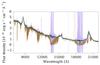 |
Fig. 1 Telluric correction for quasar SDSS1431+0535 where brown is the uncorrected spectrum and purple is the corrected spectrum and teal is the corrected spectrum smoothed by 50 pixels. The regions of pure noise are where the atmospheric transmission is ~zero, thus only leaving noise after correction. Residuals after correction are visible. The noise image is corrected correspondingly and regions severely affected are down-weighted in the weighted combination. |
From observations of a telluric standard star it is possible to calculate the atmospheric transmission spectrum by modeling the intrinsic stellar spectrum. The transmission spectrum is the fractional difference between the model and the observed spectrum. We model the telluric standard by finding the optimal linear combination of templates among the model atmospheres from the Göttingen Spectral Library (Husser et al. 2013). Here the PHOENIX model stellar atmosphere code is used to create a grid of synthetic spectra in terms of effective temperature, metallicity and alpha element enhancement. To find the optimal template we simultaneously fit for the instrumental profile broadening, velocity shift and optimal template using the penalized-pixel fitting software pPXF (Cappellari & Emsellem 2004). For the fitting we exclude all regions of strong telluric absorption since we only want to trace the stellar features. After a transmission spectrum has been constructed from the telluric standard observations, the object observation closest in time is divided by the transmission, thus correcting the absorption. As can be seen in Fig. , the intrinsic object spectrum is recovered relatively well. The regions where the continuum of the telluric standard is not found accurately will produce an erroneous transmission correction and introduce an error in the resulting corrected spectrum. We review the consequences of this in Sect. 6.4.
4. Composite construction
There is no unique way to construct a composite and the final result is influenced by the method employed. In the following we describe how the composite is constructed in this work.
4.1. Determining the redshift
Of crucial importance for the accuracy of the composite is determination of precise redshifts to accurately move the objects to the rest frame. Getting the systemic redshift of quasars from emission lines is complicated by the complex physical structure of the broad line regions in which the broad emission lines are emitted. For the bright quasars selected for our composite many of the prominent high-ionization lines visible will arise in hot clouds with high peculiar velocities and will therefore be affected by systematic line shifts (Tytler & Fan 1992; Richards et al. 2002b; Gaskell & Goosmann 2013). To get a redshift closer to the systemic we choose [O iii]λ5007, arising in the narrow-line region and therefore less affected by systematic offsets (Hewett & Wild 2010). [O iii]λ5007 is situated on a broad Fe-complex and slightly blended with [O iii]λ4959 and Hβ, with Hβ containing both broad and narrow components. This makes it difficult to model the entire emission complex by the three lines alone and therefore only the narrowest component of the [O iii]λ5007-line is used for the fit. This is similar to what is done in Vanden Berk et al. (2001). We mark both sides of the line belonging to [O iii]λ5007 where it starts to become blended, fit a low order polynomial to the edges and subtract the estimated pseudo-continuum. We define a Gaussian in terms of the rest wavelength of [O iii]λ5007 and leave the redshift as a free parameter and fit to the selected region where a weighted minimization of the residuals is done using least squares. The best-fit value and the confidence intervals on the best-fit parameters is determined by resampling the spectrum within the errors and repeating the continuum estimation and the fit on the resampled spectrum 10 000 times. The weights used are the inverse variance,  , where σ is the associated error spectrum. The 1σ confidence intervals on the fit parameters are set by the 16th and 84th percentile of the resampling realizations. Least squares minimization does not guarantee that the global minimum of the residuals will be found, but we check visually that the fits are satisfactory. [O iii]λ5007 is visible in all of our spectra in varying strength so additional refinement is not needed. As a starting guess for the redshift we use redshifts queried from SDSS and all fits are visually inspected to check if the fitted redshift is an improvement on the position of [O iii]λ5007. We show a fit to [O iii]λ5007 in Fig. , where Hβ, [O iii]λ4959 and [O iii]λ5007 are clearly detected and marked on the plot with vertical dashed lines. We transform all redshifts to barycentric standard of rest for consistent comparison with SDSS. For all of our spectra we find slight corrections to the SDSS redshifts, based on the fit to [O iii]λ5007, as is also shown in Table . We note that only one out of seven redshifts agree within the errors, but stress that the measured redshifts are not measured in a consistent manner and therefore offsets are expected. SDSS spectral redshift determinations are based on rest frame UV lines, which are known to exhibit substantial velocity shifts relative to the systemic redshift (Tytler & Fan 1992; Hewett & Wild 2010). The wavelength calibration is accurate to within 1 pixel (Krühler et al. 2015), which translates into a redshift error ≲3 × 10⁻⁵, less than reported errors.
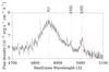 |
Fig. 2 Gaussian fit to [OIII]λ5007 for the object SDSS1354-0013. The red solid line is the linear least squared best fit. Gray dashed lines indicate the position of neighboring lines at the redshift of [OIII]. Only every 10th data point is shown for clarity. |
4.2. Galactic extinction correction
The spectra are all corrected for Galactic extinction. Extinction values are queried from the reddening maps of Schlegel et al. (1998) using the recalibration from Schlafly & Finkbeiner (2011). Extinction values in a 1.5 arcmin radius around the source are extracted from the map yielding four pixels from which an arithmetic average is taken. The reddening law by Fitzpatrick (1999) with optical total-to-selective extinction ratio RV = 3.1 is used to deredden each spectrum. The average value of the reddening for our objects is low, E(B−V) = 0.033, so we expect any residual effect of the Galactic extinction to be minimal.
4.3. Resampling
Before combination of the spectra can be done, the spectra are moved to the local frame. Because of the varying redshifts of the objects, the spectra will have their spectral arms of X-Shooter overlap at different wavelengths and will therefore have varying sampling. X-Shooter, being a cross-dispersion echelle spectrograph, has a non-linear dispersion solution and in order to conserve the most information without oversampling, we need to choose a representative bin size on which to resample our spectra. The largest sampling is in the NIR arm and is 0.6 Å/pix. An average redshift of zavg = 1.6 gives us the conservative bin size of 0.4 Å/pix in the rest-frame. Since our spectra have significantly better resolution than the nominal values and the UVB and VIS arms have a sampling of 0.2 Å/pix we will discard spectral information to make sure that we are not oversampling. We create a wavelength grid from 1000–11 350 Å in steps of 0.4 Å, giving ~16 000 spectral elements. The input spectra are moved to the rest-frame by dividing the wavelengths with (1 + z) and to conserve flux we multiply the flux density with a corresponding (1 + z). The spectra are then interpolated using a linear spline and resampled onto the newly defined common wavelength grid. Since the constituent spectra have different sampling than the target grid, we will introduce additional correlations between neighboring pixels. The high S/N ratio of the individual spectra combined with a goal to find a spectral slope over a very wide wavelength range implies that the interpolated pixel-to-pixel uncertainties does not affect the final results.
4.4. IGM absorption correction
At redshifts higher than z ~ 1.6, the rest-frame coverage of X-Shooter reaches blueward of Lyα and these spectra are therefore affected by Lyα-forest absorption, blueward of the Lyα-line. A common way to correct for this absorption is to obtain a spectrum at a sufficiently high resolution to be able to trace the continuum emission by visual inspection. At z< 2 the Lyα forest absorption is not yet heavily blended (Dall’Aglio et al. 2008), and the X-Shooter resolution allows us to effectively trace the continuum. To recover the continuum we insert points blueward of Lyα where the continuum is visually estimated. We then manually delete points that are not sufficiently smoothly varying, signifying points affected by Lyα-forest absorption. When the points represent the visually estimated continuum, a linear spline is the used to interpolate between the points onto the sampling of the original wavelength array. We then concatenate this new continuum estimate with the original spectrum, at Lyα. The objects SDSS1150-0023, SDSS1236-0331 and SDSS1431+0535 are the ones contributing the composite at these wavelengths.
4.5. Normalisation
Before combination, the spectra needs to be normalized. Depending on the type of features we are interested in and on the combination method employed, there are different ways to achieve this normalization. A popular way to normalize is to order the spectra in increasing wavelength, starting with the lowest redshift, and scale the entire spectrum by the median value of the flux and in the overlapping region with the next spectrum. The spectra are then combined consecutively, always scaling to overlapping region. The region chosen and the order of combination will affect how the final spectrum will look (Francis et al. 1991; Brotherton et al. 2001; Vanden Berk et al. 2001; Glikman et al. 2006). We choose a different normalization method. In principle the variance of the composite at each pixel should reflect the intrinsic variability of constituent spectra, but the region to which we scale will affect the absolute scale of the variance. To make the variance reflect the intra-spectral variability the most, the spectra have been scaled in the region with the least intrinsic continuum variability, which decreases with wavelength, at least up to 6000 Å (Vanden Berk et al. 2004). The region closest to 6000 Å free of contaminating emission is just redward of Hα in the region 7000–7500 Å. Each spectrum has been divided by the median flux in this region and therefore the order in which the combination is done does not matter. Before combination, all spectra have been run through a filter where if the change between neighboring pixels is greater than 10 percent, the pixel is flagged as bad and excluded from the combination. Consecutive comparison is carried out between pixels in order of ascending wavelength. This filtering algorithm is applied to exclude noisy pixels that remain in the spectra after the pipeline processing and pixels affected too strongly by residuals from the telluric absorption correction. We have investigated whether this exclusion changes the shape of the combined continuum and no effect was visible. This way of flagging noisy pixels ensures that we retain as much signal as possible without introducing very noisy isolated pixels. As many as 5 percent of the total number of pixels are rejected in the worst case.
4.6. Combination
Choosing the right combination method is important and different methods can yield slightly different results. The first assumption is that at each pixel of the composite, the constituent spectra have a Gaussian distribution around a sample mean and that this mean reflects the expectation value of the sample. Since we have a relatively small sample, even investigating whether we are sampling from a Gaussian distribution is ambiguous. To make a test for normality, we take the mean value of 100 pixels along each on the constituent spectra and, assuming that the continuum is flat in the region chosen, make a quantile-quantile plot, shown in Fig. . Given that the constituent spectra are normally distributed, the blue points should fall on the red line. From Fig. it is not immediately evident if we are sampling from a normal distribution, but it cannot be excluded. We run a Shapiro-Wilk test where the same 100 pixels from the central part of the spectrum are used. On each individual collection of pixels the test gives us a p-value for the hypothesis test, under the null hypothesis that the sample comes from a normal distribution. With an average p-value over the pixels of p = 0.55 we can at least not reject, that we are sampling from a normal distribution. Since we have no prior reason to expect that we are sampling from a Gaussian distribution and that the distribution is expected to change with wavelength increasing in width as the distance to the normalization region increases, a certain amount of caution is warranted.
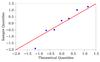 |
Fig. 3 Quantile-quantile plot as a test for normality. An average over 100 pixels in the central regions where the continuum is assumed to be relatively flat is used. The inverse cumulative distribution for the sample is constructed and plotted against the corresponding quantiles for a normal distribution. The red line arises if we are sampling for a normal distribution. Since the points are slightly steeper, this indicates a more dispersed distribution. |
In the case of uncorrelated pixels the minimal variance point estimation for the sample mean is the inverse variance weighted mean, given again that the constituent spectra at each wavelength bin can be treated as stochastic variables that follow a normal distribution  with mean μ and variance
  . The inverse variance weighted mean is calculated as
 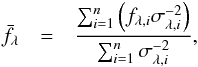 (1)with the variance of the weighted mean given as
  (2)Because we have resampled the pixels to a common pixel scale, additional correlation between adjacent pixels will be introduced both in the flux spectrum and in the error spectrum, meaning that we will underestimate the errors in the resulting composite spectrum where the missed statistical noise will be hiding in pixel-to-pixel variations. Additionally, since our objects are fairly bright, the Poisson noise in our spectra will be non-negligible and thus we are incorporating the pixel values themselves into their weights, which leads to a bias in the result toward spectra of lower signal-to-noise. We check how the combination method employed affects the qualitative features in our spectrum in Sect. 6.4.
4.7. Absolute magnitudes
In order to make a meaningful comparison with other composites and to the parent population of quasars, synthetic apparent magnitudes are calculated and then, using the redshift, converted to absolute magnitudes. Synthetic photometry is the process by which the apparent magnitudes in a bandpass is obtained from a spectrum by convolution with the filter quantum efficiency curve (Bessell 2005). Following Bessell & Murphy (2012) and Casagrande & VandenBerg (2014) we calculate the synthetic AB magnitudes using  (3)where fλ(λ) is the observed flux density in units of erg s-1 cm-2 Å-1 for the spectra and Tx is the total system fractional throughput in band x. The apparent magnitude can then be converted to absolute magnitude using
 ![Mathematical equation: \begin{eqnarray} \label{absmag} M_{\textmd{AB}_x} &=& -5 \log_{10} \left[\frac{D_{\rm L}}{10~\mathrm{pc}} \right] + m_{\textmd{AB}_x} , \end{eqnarray}](/articles/aa/full_html/2016/01/aa27096-15/aa27096-15-eq52.png) (4)with the luminosity distance, DL, calculated using a standard cosmological calculator1. Using the SDSS i-band filter transmission curve2, interpolated to the spectral element size, we get the absolute i-band magnitudes, Mi(z = 0). The largest compilation of quasar absolute magnitudes to date is Pâris et al. (2014), in which the K-corrected, i-band magnitudes normalized at z = 2, Mi(z = 2), for the 166 583 quasars in DR10 are presented. To get the corresponding magnitudes for the composite constituent quasars at z = 2, we follow the prescription from Richards et al. (2006b) in which the absolute magnitude for an observer at z = 0 is converted to that of an observer at z = 2. This is done to minimize the systematic effect on the magnitude of the K-correction arising from the varying continuum slopes of quasars. The farther away that a given quasar is from the normalization redshift, the greater the error from a wrongly assumed continuum slope. Choosing z = 2 as the normalization redshift, which is close to the peak in quasar number density as a function of time (Richards et al. 2006b; Hopkins et al. 2007), minimizes this error. We have not substituted the assumed slope of α = 1.5 with the updated value, for consistency with the comparison sample.
(4)with the luminosity distance, DL, calculated using a standard cosmological calculator1. Using the SDSS i-band filter transmission curve2, interpolated to the spectral element size, we get the absolute i-band magnitudes, Mi(z = 0). The largest compilation of quasar absolute magnitudes to date is Pâris et al. (2014), in which the K-corrected, i-band magnitudes normalized at z = 2, Mi(z = 2), for the 166 583 quasars in DR10 are presented. To get the corresponding magnitudes for the composite constituent quasars at z = 2, we follow the prescription from Richards et al. (2006b) in which the absolute magnitude for an observer at z = 0 is converted to that of an observer at z = 2. This is done to minimize the systematic effect on the magnitude of the K-correction arising from the varying continuum slopes of quasars. The farther away that a given quasar is from the normalization redshift, the greater the error from a wrongly assumed continuum slope. Choosing z = 2 as the normalization redshift, which is close to the peak in quasar number density as a function of time (Richards et al. 2006b; Hopkins et al. 2007), minimizes this error. We have not substituted the assumed slope of α = 1.5 with the updated value, for consistency with the comparison sample.
5. Results
We show the weighted mean composite in Fig. . Characteristic features of quasars are readily visible. We see several prominent emission lines across the entire spectral range, which includes both very broad high-ionization lines and narrower low-ionization lines as is typical of quasar spectra, with both broad and narrow lines superposed with multiple components (Baldwin et al. 1995). We have marked the position and name of the most prominent lines and overplotted them in Fig. . Analyses of the lines are beyond the scope of this paper.
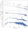 |
Fig. 4 Top panel: composite spectrum with prominent emission lines marked. Upper middle panel: measure of intra-spectrum variability. The standard deviation of the constituent spectra as a function of wavelength, where to normalize the differing slopes between the different spectra, the fitted slope in each of the constituent spectra have been subtracted. Lower middle panel: signal-to-noise ratio. The composite spectrum is divided by the error spectrum, thus directly giving a measure of the signal strength. Bottom panel: number of contributing spectra as a function of wavelength. |
As is often seen, the continuum level is shrouded by a myriad of emission lines, Balmer continuum and Fe-complexes scattered across the entire spectrum, making the intrinsic shape of the continuum difficult to estimate (Elvis 2001). The composite spectrum covers from Lyβ in the bluest part of our spectrum to Paγ in the reddest, where a power law adequately describes the continuum from Lyα and redward. Blueward of Lyα, the spectral continuum changes slope toward a shallower spectral slope. The change in slope is a consequence of the accretion disk mechanism responsible for the continuum emission where the position of the spectral break is set by the temperature of the accretion disk (Pereyra et al. 2006). The correction for Lyα-forest absorption is described in Sect. 4.4. Between ~2000 Å and ~5000 Å, excess emission compared with a pure power law is detected, consistent with the small blue bump (Wills et al. 1985), which consists of a blend of Balmer continuum and Fe ii lines, with both broad and narrow components.
The continuum of a single quasar spectrum is usually modeled as a power law, fλ ∝ λαλ, but a weighted mean spectrum of a sample of power-law continua does not, in general, result in a power law with a slope equal to the mean slope of the individual quasar spectra. In principle, a geometric mean of a sample of power laws should result in a power law with a spectral index being the mean of the individual spectral indices, as is shown in Appendix A. We compare the composite obtained by taking the geometric mean with that obtained by the weighted average and no significant difference is detected between the two composites. We therefore take the weighted mean composite as representative of the constituent spectra. This potential cause of systematic error due to combination methods is investigated more in Sect. 6.4.
Regions free of contaminating line emission are very scarce and fitting a power law to the composite in manually specified regions is not guaranteed to reflect the spectral index of the continuum. A quantitative measure of the shape can be obtained by carefully selecting regions that appear relatively unaffected by line emission in excess of the continuum. The regions that cover the widest wavelength range are: 1300–1350, 1425–1475, 5500–5800, 7300–7500 Å, which we use to fit both with a single power law and a broken one, with a break redward of Hβ at 5000 Å as is reported by other authors (e.g., Vanden Berk et al. 2001). For the single power law we obtain αλ = −1.70, where for a broken power law, we obtain a spectral index αλ = −1.69 below 5000 Å, and αλ = −1.73 above, consistent with a single power law describing the continuum from Lyα to Paγ. The break in Vanden Berk et al. (2001) is attributed to contamination from the host galaxies (Glikman et al. 2006) and adapting the same interpretation, gives support to the assumption about the negligible host galaxy contribution present in the composite presented here. A detailed comparison with existing composites is done in Sect. 2.
5.1. Applicability of the composite
To test the applicability of the composite, it is used to determine the dust content of a sample of three red quasars taken from the High AV QSO (HAQ) survey (Krogager et al. 2015). The HAQ survey consists of quasars selected on the basis of their optical colors in SDSS and near-infrared in UKIDDS to identify the reddest and therefore most dust-extincted quasars which are missed by traditional color selection criteria. A complete description of the sample criteria and the data are presented in Fynbo et al. (2013) and Krogager et al. (2015). The dust content is inferred by reddening the composite with an extinction law parameterized by Gordon et al. (2003) to match the object spectrum. The parameterization allows the redshift of the object quasar and the magnitude of visual extinction, AV, to be found by minimizing the residuals between the object and the composite. A detailed description of the fitting method is given in Krogager et al. (2015). The three quasars have been selected to have varying amounts of extinction and have differing redshifts. We show the result for quasars HAQ2221+0145, HAQ1115+0333 and HAQ2231+0509 in Fig. where the success of matching the composite with quasars of very different shapes is visible. Following Wang et al. (2012), the previous composite used to fit for the dust amount consists of the composite generated by Vanden Berk et al. (2001) stitched together with the composite by Glikman et al. (2006) at 3000 Å. Thus, two different composites built from differing samples have been treated as a single composite. That this has been successful is a testament to the similarity of quasars across a wide range of apparent physical conditions. The values obtained with our composite is entirely consistent with the values published in Krogager et al. (2015), which is encouraging for the previous use of the stitched template. A detailed comparison between the different composites is presented in Sect. 2.
There exists a distribution of slopes for quasar continua and when using the composite presented here, the intrinsic slope of the modeled quasar is highly degenerate with the amount of dust inferred (Reichard et al. 2003). Since attenuation by dust is stronger at shorter wavelengths, extinction introduces a curvature in the spectrum, which is separate from a pure change in slope, see Krawczyk et al. (2015) for a discussion of red vs. reddened quasars.
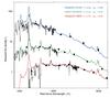 |
Fig. 5 Dust extinction, AV, and redshift has been inferred for three HAQ quasars by fitting for the amount of reddening required to match the template with the observed spectrum. The black spectra are taken at the Nordic Optical Telescope (NOT) using the ALFOSC spectrograph. The black squares are optical ugriz photometric points from SDSS and UKIDSS YJHK bands. For varying amount of extinction at different redshifts, consistent results are found with previous usage of stitched composites. |
5.2. Intra-spectrum variability
To gauge the intra-spectrum variability, the power-law slope of each individual spectrum is subtracted from the flux points at each wavelength thereby removing the variability due to different slopes. The standard deviation is then taken of the normalized spectra, which then reflects the variability of the spectra around the composite. We show the computed normalized variability in Fig. . The normalized sample variability contains both the temporal variability and the intrinsic population variability, which is not possible to separate with single-epoch data. Significant variation is visible in the lines of C iv, Mg ii, [O iii]λ5007 and lines of hydrogen as well as in the Fe ii-complexes centered on Hβ. From C iv to Hβ an increase in continuum variability is observed, likely due to the quasar-to-quasar variability of the small blue bump. In the region blueward of Lyα the fractional variability reaches 60 per cent, attributed to the stochastic nature of the Lyman-α forest.
6. Discussion
The applicability of quasar composites as tools for template matching and dust estimation largely hinges on the ability of the composite to represent an intrinsic target spectrum. The broad usage and success of previous composites largely confirms this ability. That the constructed composites are representative of a large group of differently selected quasars is a testament to the homogeneity of the quasar population and the universality of the emission mechanism. The remarkable uniformity of the average spectral properties across luminosity and redshift indicates very similar underlying physical mechanisms that can be understood in terms of Eigenvector 1 (Boroson & Green 1992; Francis et al. 1992) where the Eddington ratio drives the relative strength of the lines, and orientation effects influences the observed kinematics of the lines (Shen & Ho 2014). The specific local physical conditions that regulate the accretion rate then account for the majority of the inter-quasar variation. In this section, we will investigate whether the targets selected are simply scaled-up version of average quasars, or remarkable in some sense.
6.1. Comparison to global population
The QSOs selected for this study lie amongst the brightest values of Mi(z = 2) compared to the spectroscopically confirmed SDSS QSOs (Shen et al. 2011), which are uniformly selected to ~90 percent completeness (Richards et al. 2002a; Vanden Berk et al. 2005). It is clear that the sample presented here represents some of the brightest quasars existing between redshift 1 and 2. It is therefore potentially a biased subset of the global quasar population. Quasars have previously been shown to exhibit a high degree of homogeneity over many orders of magnitude (Dietrich et al. 2002), but this is only true for quasars resembling average quasars and not exotic sub-types. To ensure that the targets selected for this sample are not outliers in color, the spectrophotometric colors are compared to those of the quasar population presented in Pâris et al. (2014)3. We show the comparison in Fig. . From the magnitudes, we first confirm that the quasars selected here are among the intrinsically brightest visible in i-band with a 2.7 sigma magnitude distance from the mean absolute i-band magnitude, normalized at redshift 2, Mi(z = 2) of the full SDSS quasar catalog for DR10. Despite their luminosities the colors are representative of the subset fulfilling the selection criteria. As a consistency check, the composite generated in this work is used to fit for the dust content of quasars with varying degree of extinction and consistent results were obtained as compared with composites generated from other subsamples of the parent population. For a comparison between SDSS and quasars detected in GALEX, UKIDSS, WISE, 2MASS and Spitzer, see Krawczyk et al. (2013).
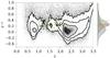 |
Fig. 6 Quasar color, g−i, as a function of redshift, z. The full quasar sample from SDSS DR10 (Pâris et al. 2014) is shown in gray color. Bounding contours show the 0.5, 1, 1.5, 2σ contours of the density of points. The olive points are individual quasars from the SDSS sample which satisfy r< = 17. Overplotted in pink are the quasars contributing to the composite presented here. The quasar colors have been marginalized over in the right side where the tall pink lines are at the position of the composite quasars and the olive shaded area is the kernel density estimation of the distribution of quasars fulfilling the selection criteria. The gray-shaded area is the projection of the DR10 quasar sample. |
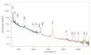 |
Fig. 7 X-Shooter weighted arithmetic mean quasar composite on a linear wavelength scale in light brown. The positions of several prominent emission lines are marked. Overplotted in dark green is the corresponding composite generated from the full sample of SDSS quasars fulfilling the selection criteria and general agreement is observed, albeit with a brighter Balmer continuum in the SDSS-constructed composite. In purple is shown the results from fitting both a pure and a broken power law to the regions specified in Sect. 5 and they are observed to be indistinguishable. |
Because of the high luminosity of the objects presented here, several differences in the properties are expected as compared to those of the global quasar population. The physical scales locally are expected to be larger (Bentz et al. 2013), which will make variability timescales longer and variability magnitudes smaller (Vanden Berk et al. 2004; Schmidt et al. 2012). Black-hole masses as determined from Mg ii increases with luminosity (Wu et al. 2015) which in turn affects the temperature of the accretion disc (Shakura & Sunyaev 1973; Pereyra et al. 2006) and thereby the position of the “big blue bump” and the degree to which the continuum is well modeled by a single power law (see also Lusso et al. 2015, for a discussion). As can be seen from Fig. , the quasars selected for the composite represent average colors for the subset fulfilling the sample cuts. An immediate consequence of this will be that the amount of dust inferred using this composite will be an average content over a statistical sample, because the individual object which is sought modeled, can have an intrinsic quasar continuum shape that is different from what is constructed here (Richards et al. 2003; Hopkins et al. 2004). Populations with intrinsically different spectral slopes exists (Glikman et al. 2012; Krawczyk et al. 2015) and the bias in the inferred amount of extinction is therefore larger in these types of surveys. Since the true intrinsic dereddened quasar color distribution is likely broad with a range of slopes, a caveat of using this composite is that the amount of extinction inferred will be the average amount over a large sample.
6.2. Comparison to the sample population
Because of the low number statistics used for the sample presented in this work, a further bias can be that the targets are not representative of the population fulfilling the cuts imposed in the selection. As highlighted in Fig. , the objects selected here are comparable in color to the full sample fulfilling the selection criteria. To quantify the bias against the selection, we construct a composite in an identical fashion consisting of all SDSS quasars fulfilling the selection criteria. In Fig. we overplot the composite generated from the SDSS spectra of the full sample fulfilling the selection criteria on the one constructed with X-Shooter. It is clear that there are small differences in the shape of the composite constructed from the full sample and the small sample, but qualitatively the shape remains the same. Calculating the power-law slope in each individual SDSS spectrum yields αλ = −1.6 ± 0.3, but this number is difficult to interpret due to the narrow continuum region free of emission lines (1300–1350 Å and 1425–1475 Å). It is reassuring nonetheless that they are consistent within the errors as seen in Table . We investigate the effect of a finite sample size on the combination method in Sect. 6.4.1.
6.3. Comparison to existing composites
We compare the X-Shooter composite to composites from the literature by the following authors: Francis et al. (1991), Vanden Berk et al. (2001), Telfer et al. (2002), Glikman et al. (2006) and Lusso et al. (2015). Francis et al. (1991) generated a composite from 688 LBQS (Large Bright Quasar Survey)-quasars observed mainly with the Multiple Mirror Telescope (MMT). The absolute magnitudes cover ~−22 and ~−28 at a redshift range 0.05 <z< 3.36 subject to a significant Malmquist bias for which the mean absolute magnitude is a strong function of rest-frame wavelength, with the brightest objects contributing at shortest wavelengths and visa versa for the faint objects. The composite by Vanden Berk et al. (2001) consists of 2204 SDSS quasars at zmedian = 1.253 with absolute Mr′-magnitudes between −18.0 and −26.5 and therefore intrinsically fainter and lower redshift objects. Lusso et al. (2015) calculated the Mi(z = 2) mag for the 184 constituent objects in Telfer et al. (2002) observed with FOS, GHRS and STIS onboard the Hubble Space Telescope and find an average Mi(z = 2) ~ −27.5 at z ~ 1.2, which yields a composite of fainter, more nearby sources. For construction of a composite, Glikman et al. (2006) used 27 objects at z ~ 0.25 with an average absolute i-band magnitude Mi ~ −24 observed with IRTF, therefore constituting a fainter, lower redshift sample. Lastly, Lusso et al. (2015) used 53 quasars observed with WFC3 at z ~ 2.4 with absolute i-band magnitudes at redshift 2, Mi(z = 2) ~ −28.5, so of comparable brightness, but at slightly larger distances.
Regardless of the variation across selection criteria, luminosities and redshifts, a remarkable similarity in the overall shape is visible over a wide wavelength range. The simultaneous existence of lines arising in such different environments around objects differing by many orders of magnitude in luminosity is caused by the varying conditions in the emitting clouds which ensure that each ionic species has optimal conditions to produce line emission (Baldwin et al. 1995). Significant differences between the composites are visible blueward of Lyα where different methods for IGM absorption correction has been employed. No correction has been applied in the composites by Francis et al. (1991) and Vanden Berk et al. (2001) and a sharp decrease in continuum flux is detected. Because higher redshift objects contribute mostly at shorter wavelengths, significant Lyα absorption is expected regardless due to the Lyα opacity evolution (Moller & Jakobsen 1990; Madau 1995; Dall’Aglio et al. 2008). The IGM correction of Telfer et al. (2002) is a hybrid in which some manual and some statistical correction has been applied. Lusso et al. (2015) rely on a purely statistical correction that is calculated by integrating the neutral hydrogen column density distribution at z ~ 2.4 measured by Prochaska et al. (2014). The IGM correction in the X-Shooter composite presented here is done in each individual spectrum where resolved lines are interpolated over. Good agreement is found in the Lyα forest region with Telfer et al. (2002), but underestimated as compared to Lusso et al. (2015), which can be seen in the insert in Fig. . As argued by Lusso et al. (2015), an explanation for this discrepancy is the underestimation of the correction needed to account for unidentified Lyman limit absorbers. Due to the resolution of the instrument and the redshifts probed, this should not be a significant effect on the sources observed here. Differences in the emission lines are also visible. This is to be expected due to the highly varying magnitudes of the constituent objects for the different composites where a decreasing equivalent line width is expected with increasing luminosity (Baldwin 1977). Above 5000 Å, a clear discrepancy is visible to the Vanden Berk et al. (2001) composite which is due to host galaxy contamination (Glikman et al. 2006). From the quasars in DR7 (Shen et al. 2011), it is confirmed that this effect is not affecting the X-Shooter composite presented here to a significant degree, due to the extreme luminosities. This is investigated further in Sect. 6.4.6.
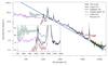 |
Fig. 8 Comparison of different composites. The composites by Lusso et al. (2015), Vanden Berk et al. (2001), Telfer et al. (2002), Francis et al. (1991) are normalized to the X-Shooter composite at ~1450 Å and the composite by Glikman et al. (2006) is normalized to ours at ~3850 Å. Significant differences are visible blueward of Lyα due to differing IGM correction methods. Above 5000 Å significant host galaxy contamination is visible in the composite by Vanden Berk et al. (2001). Overplot in blue is a power law with slope αλ = −1.70 and normalized at ~1450 Å. |
Power law slopes from different composites.
Despite the similarity visible in the direct comparison, it is remarkable that the power-law slope blueward of 10 000 Å is found to be varying by more than 30 per cent between the different authors. We compile the results from the different composites in Table . One likely reason for the discrepancies is the wavelength regions used for the continuum where an increased wavelength coverage allows a better continuum to be selected, especially selecting regions unaffected by Balmer continuum and broad Fe ii complexes. A more direct comparison of the slopes, where an explicit fit to the same regions is made, is not possible due to the different wavelength coverage. A narrow region free of line emission just redward of Lyα is covered by most of the composites in the comparison, but fitting a power law to such a narrow region for a small sample would largely leave the inferred slope dependent on the exact ranges chosen for the fit.
6.4. Systematics
Understanding how systematic effects may affect results is important in making robust conclusions. We list the possible systematics that effect the composite and address each of the points separately to investigate to what degree they affect the final result and their potential consequences.
6.4.1. Combination method
What is sought illustrated with the combination method employed is the central tendency of the selected sample normalized at an optimally chosen region. Since the underlying distribution is unknown, choosing the optimal point estimator for the average flux value is ambiguous. The composite presented in Sect. 5 used the weighted arithmetic mean, which was chosen because it is the maximum likelihood estimator of the mean, given that we are sampling from a normal distribution with independent sampling. This combination method, however, has systematic differences from other methods, especially the danger of biasing the composite toward the highest signal-to-noise spectra.
To test whether we are biased toward high S/N spectra we compare the weighted mean spectrum with the composite created from the median. We perform the comparison by constructing a fractional difference spectrum, which is a ratio between the two composites. There is very good agreement between the two composites with a mean fractional difference of 0.01 ± 0.05 per cent. There are no observed trends with wavelength.
The systematic error in the reported slope due to the different combination methods is assessed by fitting a single power law in the same regions as in Sect. 5 for each combination method and in the constituent spectra. The value of the spectral indices, αλ are shown in Table for the different composites. The value of and error on the slope is obtained by resampling the spectra within the errors and refitting a power law for each realization. The errors used for resampling are the standard deviations of the constituent spectra at each spectral bin and, where available, the statistical errors are added in quadrature. A weighted least squares fit is performed on the 10 000 realizations, and the best-fit value is taken as the mean of the fitted slopes. The reported error is the standard deviation of the sample of inferred slopes. The error on the composites should approach the one reported for αλ measured on the individual spectra which reflect the intrinsic variability of slopes. The standard deviation of the individual slopes is more reasonable and all combination methods are consistent within these errors. The values for the individual mean and individual median differ by a small amount and this could suggest a slight skew in the distribution of slopes, but the low level of discrepancy could also be an artifact of low number statistics. The fact that the fitted slopes are consistent supports the use of the weighted mean composite.
In general the arithmetic mean spectrum is not guaranteed to have a slope with the mean spectral index ⟨ aλ ⟩ of the individual spectra, see Appendix A, but what we see here is a very good agreement. To obtain a spectrum with the mean slope of the individual spectra, the geometric mean does give rise to a slope equaling the mean slope. The low level of discrepancy between the different methods is encouraging to the use of the weighted mean.
6.4.2. Selection effects
Bright quasars with (r ≲ 17) at redshifts 1 <z< 2.1 are not necessarily representative of the intrinsic quasar population (Pâris et al. 2014) and the final composite is not guaranteed to reflect the properties of quasars at different magnitudes or redshifts. Comparison to the parent population yields, in terms of colors, a redder than average selection for the quasars fulfilling the selection criteria for the X-Shooter composite. The objects that fulfill the selection criteria are ~0.2 mag redder than the quasar mean g−i color. This translates into changing a pure power-law slope from −1.6 to −1.9, so toward steeper slope and more blue spectra. Since quasar spectra are more complicated than pure power laws, a more likely explanation for this offset between the full quasar sample and the subset selected here is the shifting of Lyα-line emission into the SDSS g-band, therefore artificially making the continuum appear bluer. A comparison to the composite by Vanden Berk et al. (2001) which consists of lower redshift, intrinsically fainter quasars, shows a high degree of similarity in the general shape and small differences on small scales, see Sect. 2.
6.4.3. Flux calibration
Power law slopes from different combination methods.
As stated in Sect. 3, we find slight variations in both the absolute flux level and spectral slope of the X-Shooter observed spectra compared with those observed with SDSS. Since we are to a high degree seeing limited, we expect the slit loss to be insignificant and potential alternative solutions are investigated. To quantify this effect of variation of the accuracy of our flux calibration compared with the corresponding object spectra obtained with SDSS, we compare the photometry obtained from SDSS with the synthetic magnitudes calculated in Sect. 4.74. We calculate the mean difference between the two magnitudes. There is a clear trend with highest deviations in the u-band and a monotonic decrease in deviations toward z-band, with −0.4 ± 0.3 mags in the u-band to −0.1 ± 0.2 mags in the z-band. This variation is caused by both the accuracy of the flux calibration and the intrinsic quasar variability. Since the slit loss is expected to be wavelength dependent, peaking in the blue, this is consistent with the trend observed. For the intrinsic variability, MacLeod et al. (2012) find a characteristic variation timescale of ~2 yr with an average rest-frame variation of ~0.26 mag – comparable to what is observed here. Recent work by Morganson et al. (2014) confirm the results of Helfand et al. (2000) that quasars are more variable in bluer bands – also consistent to what is found here. Since the mean temporal deviation should average to zero and we find negative mean differences, part of the discrepancy is likely attributed to flux calibration differences. It is difficult to attribute the total variation to either explanation.
6.4.4. Normalization region
Depending on the region selected for normalization of the individual spectra, the distribution of constituent fluxes at any given wavelength changes. This will mostly affect the absolute scale of the composite and the reported inter-spectrum variability as a function of wavelength, but will also cause the value of the composite at a given wavelength to change depending on the choice of central tendency estimator. To investigate how the normalization-window chosen affects the shape of the composite, we have generated composites for varying position of the normalization-window across the entire wavelength range. We have chosen regions clear of strong emission lines. The different combination methods yield slightly varying composites as the relative distribution of the fluxes changes for a changing normalization region. After rescaling the composites to unity at 6850 Å we see very good agreement between the different normalization regions.
We fit a power-law slope to composites generated with varying normalization regions and take the standard deviation of the fitted slopes as the 1σ systematic error due to different normalization regions and find a value of: σn = ± 0.03.
6.4.5. Telluric correction
To test the magnitude of the noise introduced by the telluric correction we construct a composite where instead of correcting for the atmospheric absorption we exclude regions of low transmission, namely the two absorption band at ~14 000 and ~19 000 Å. The effect on the composite is largely an increase in noise in the regions where individual spectra have been masked, but more problematic is the introduction of residual atmospheric absorption in unmasked regions. Since there is significant absorption from ~7000 Å and redward, as is also visible in Fig. , and especially in the NIR arm, masking each individual absorption complex throughout the spectrum is not desirable. The telluric correction method essentially leaves the unaffected region free of change.
6.4.6. Host galaxy contamination.
A geometric composite has been generated in bins of luminosity by Shen et al. (2011) and the evolution of the relative contribution from the host galaxy with luminosity is investigated. It can be seen that the lower luminosity quasars have a spectral break around ~4000 Å, which is lacking at higher luminosities and attributed to host galaxy contamination. We calculate L5100 for the spectra in the composite presented here, using the continuum flux density at 5100 Å and converting to luminosity following Netzer & Trakhtenbrot (2007),  (5)we find and average log L5100 = 46.7 ± 0.1 which is an order of magnitude higher than the highest luminosity bin in Shen et al. (2011) which is assumed to be free of host galaxy contamination. This is consistent with what is found by Hopkins et al. (2007), that host galaxy light is likely a small contribution for quasars brighter than MB ≳ −23. We have selected our quasars to be very bright and at high redshift thereby reducing the spectral contamination from underlying host galaxy light.
7. Conclusion
We have generated a quasar composite covering the entire range from 1000 Å to 11 350 Å based on observations with X-Shooter of seven bright (r ≲ 17) quasars at redshifts 1 <z< 2.1 free of host galaxy contamination. Assuming a power-law continuum, we found a spectral slope of αλ = −1.70 ± 0.01, which is somewhat steeper than for composites presented by other authors. We found a consistent slope within errors for various combination methods. We attributed the discrepancy between the power-law slopes to the different wavelength coverages, where the very wide wavelength coverage of X-Shooter ensures that we can effectively choose regions free of emission lines and line-continuum emission, especially the Balmer continuum and Fe ii-line complexes, i.e., the Small Blue Bump heavily affecting the region from 2000–5000 Å. We applied the composite to fit for the amount of dust in three quasars with varying dust content and found that the amount of visual extinction agrees with what is found using a combination of previously generated composites. A comparison with other composites was done, and a high degree of similarity is highlighted despite the very different selection criteria and reported spectral slopes. We have made the composite and all the code used to generate it available at https://github.com/jselsing/QuasarComposite. We show a portion of the composite values for clarity regarding the format in Table .
Quasar composite spectrum.
Astropy.cosmology.
Acknowledgments
We thank the anonymous referee for a constructive report that improved our manuscript on several important points. We thank Marianne Vestergaard and Jens Hjorth for useful discussions and suggestions. The research leading to these results received funding from the European Research Council under the European Union’s Seventh Framework Program (FP7/2007-2013)/ERC Grant agreement no. EGGS- 278202. L.C. acknowledges support from an YDUN grant DFF – 4090-00079. The Dark Cosmology Centre was funded by the DNRF. This research made use of Astropy, a community- developed core Python package for Astronomy (Astropy Collaboration 2013). The analysis and plotting has been achieved using the Python-based packages Matplotlib (Hunter 2007), Numpy, and Scipy (van der Walt et al. 2011), along with other community-developed packages.
References
- Ahn, C. P., Alexandroff, R., Allen de Prieto, C., et al. 2012, ApJSS, 203, 21 [NASA ADS] [CrossRef] [Google Scholar]
- Annis, J., Soares-Santos, M., Strauss, M. A., et al. 2014, ApJ, 794, 120 [NASA ADS] [CrossRef] [Google Scholar]
- Astropy Collaboration. Robitaille, T. P., Tollerud, E. J. 2013, A&A, 558, A33 [NASA ADS] [CrossRef] [EDP Sciences] [Google Scholar]
- Baldwin, J. A. 1977, ApJ, 214, 679 [NASA ADS] [CrossRef] [Google Scholar]
- Baldwin, J., Ferland, G., Korista, K., & Verner, D. 1995, ApJ, 455, L119 [NASA ADS] [CrossRef] [Google Scholar]
- Bentz, M. C., Denney, K. D., Grier, C. J., et al. 2013, ApJ, 767, 149 [NASA ADS] [CrossRef] [Google Scholar]
- Bessell, M. S. 2005, ARA&A, 43, 293 [NASA ADS] [CrossRef] [Google Scholar]
- Bessell, M., & Murphy, S. 2012, PASP, 124, 140 [Google Scholar]
- Boroson, T. A., & Green, R. F. 1992, ApJS, 80, 109 [NASA ADS] [CrossRef] [Google Scholar]
- Boyle, B. J. 1990, MNRAS, 243, 231 [NASA ADS] [Google Scholar]
- Brotherton, M. S., Tran, H. D., Becker, R. H., et al. 2001, ApJ, 546, 775 [NASA ADS] [CrossRef] [Google Scholar]
- Cappellari, M., & Emsellem, E. 2004, PASP, 116, 138 [NASA ADS] [CrossRef] [Google Scholar]
- Casagrande, L., & VandenBerg, D. A. 2014, MNRAS, 444, 392 [NASA ADS] [CrossRef] [MathSciNet] [Google Scholar]
- Chen, Y.-P., Trager, S. C., Peletier, R. F., et al. 2014, A&A, 565, A117 [NASA ADS] [CrossRef] [EDP Sciences] [Google Scholar]
- Christensen, L., Fynbo, J. P. U., Prochaska, J. X., et al. 2011, ApJ, 727, 73 [NASA ADS] [CrossRef] [Google Scholar]
- Cristiani, S., & Vio, R. 1990, A&A, 227, 385 [NASA ADS] [Google Scholar]
- Croom, S. M., Smith, R. J., Boyle, B. J., et al. 2004, MNRAS, 349, 1397 [NASA ADS] [CrossRef] [Google Scholar]
- Dall’Aglio, A., Wisotzki, L., & Worseck, G. 2008, A&A, 491, 465 [NASA ADS] [CrossRef] [EDP Sciences] [Google Scholar]
- Dietrich, M., Hamann, F., Shields, J. C., et al. 2002, ApJ, 581, 912 [NASA ADS] [CrossRef] [Google Scholar]
- Dobos, L., Csabai, I., Yip, C.-W., et al. 2012, MNRAS, 420, 1217 [NASA ADS] [CrossRef] [Google Scholar]
- Elvis, M. 2001, ApJ, 545, 63 [Google Scholar]
- Fitzpatrick, E. L. 1999, PASP, 111, 63 [NASA ADS] [CrossRef] [Google Scholar]
- Francis, P. J., Hewett, P. C., Foltz, C. B., et al. 1991, A high signal-to-noise ratio composite quasar spectrum, 373, 465 [Google Scholar]
- Francis, P. J., Hewett, P. C., Foltz, C. B., & Chaffee, F. H. 1992, ApJ, 398, 476 [NASA ADS] [CrossRef] [Google Scholar]
- Freudling, W., Romaniello, M., Bramich, D. M., et al. 2013, A&A, 559, A96 [NASA ADS] [CrossRef] [EDP Sciences] [Google Scholar]
- Fynbo, J. P. U., Krogager, J.-K., Venemans, B., et al. 2013, ApJSS, 204, 6 [NASA ADS] [CrossRef] [Google Scholar]
- Gaskell, C. M., & Goosmann, R. W. 2013, ApJ, 769, 30 [NASA ADS] [CrossRef] [Google Scholar]
- Glikman, E., Helfand, D. J., & White, R. L. 2006, A&ARv, 640, 579 [Google Scholar]
- Glikman, E., Helfand, D. J., White, R. L., et al. 2007, ApJ, 667, 673 [NASA ADS] [CrossRef] [Google Scholar]
- Glikman, E., Urrutia, T., Lacy, M., et al. 2012, ApJ, 757, 51 [NASA ADS] [CrossRef] [Google Scholar]
- Gordon, K. D., Clayton, G. C., Misselt, K. A., Landolt, A. U., & Wolff, M. J. 2003, ApJ, 594, 279 [NASA ADS] [CrossRef] [EDP Sciences] [Google Scholar]
- Gunn, J. E., Siegmund, W. a., Mannery, E. J., et al. 2006, AJ, 131, 2332 [NASA ADS] [CrossRef] [Google Scholar]
- Hamuy, M., Suntzeff, N. B., Heathcote, S. R., et al. 1994, PASP, 106, 566 [NASA ADS] [CrossRef] [Google Scholar]
- Helfand, D. J., Stone, R. P. S., Willman, B., et al. 2000, AJ, 121, 1872 [Google Scholar]
- Hewett, P. C., & Wild, V. 2010, MNRAS, 405, 2302 [NASA ADS] [Google Scholar]
- Hopkins, P. F., Strauss, M. a., Hall, P. B., et al. 2004, AJ, 128, 1112 [NASA ADS] [CrossRef] [Google Scholar]
- Hopkins, P. F., Hernquist, L., Cox, T. J., et al. 2006, ApJS, 163, 1 [Google Scholar]
- Hopkins, P. F., Richards, G. T., & Hernquist, L. 2007, ApJ, 654, 731 [NASA ADS] [CrossRef] [Google Scholar]
- Hunter, J. D. 2007, Comput. Sci. Eng., 9, 90 [Google Scholar]
- Husser, T.-O., Wende-von Berg, S., Dreizler, S., et al. 2013, A&A, 553, A6 [NASA ADS] [CrossRef] [EDP Sciences] [Google Scholar]
- Jiang, P., Zhou, H., Ji, T., et al. 2013, AJ, 145, 157 [NASA ADS] [CrossRef] [Google Scholar]
- Kauffmann, G., Heckman, T. M., Tremonti, C., et al. 2003, MNRAS, 346, 1055 [Google Scholar]
- Kausch, W., Noll, S., Smette, A., et al. 2015, A&A, 576, A78 [NASA ADS] [CrossRef] [EDP Sciences] [Google Scholar]
- Krawczyk, C. M., Richards, G. T., Mehta, S. S., et al. 2013, ApJS, 206, 4 [NASA ADS] [CrossRef] [Google Scholar]
- Krawczyk, C. M., Richards, G. T., Gallagher, S. C., et al. 2015, AJ, 149, 203 [NASA ADS] [CrossRef] [Google Scholar]
- Krogager, J.-K., Geier, S., Fynbo, J. P. U., et al. 2015, ApJS, 217, 5 [NASA ADS] [CrossRef] [Google Scholar]
- Krühler, T., Malesani, D., Fynbo, J. P. U., et al. 2015, A&A, 581, A125 [NASA ADS] [CrossRef] [EDP Sciences] [Google Scholar]
- Leighly, K. M., Terndrup, D. M., Baron, E., et al. 2014, ApJ, 788, 123 [NASA ADS] [CrossRef] [Google Scholar]
- Lusso, E., Worseck, G., Hennawi, J. F., et al. 2015, MNRAS, 449, 4204 [NASA ADS] [CrossRef] [Google Scholar]
- MacLeod, C. L., Ivezić, Ž., Sesar, B., et al. 2012, ApJ, 753, 106 [NASA ADS] [CrossRef] [Google Scholar]
- Madau, P. 1995, ApJ, 441, 18 [NASA ADS] [CrossRef] [Google Scholar]
- Mannucci, F., Basile, F., Poggianti, B., et al. 2001, MNRAS, 326, 745 [NASA ADS] [CrossRef] [Google Scholar]
- Modigliani, A., Goldoni, P., Royer, F., et al. 2010, SPIE Astron. Telesc. Instrum., 7737, 773728 [Google Scholar]
- Moller, P., & Jakobsen, P. 1990, A&A, 228, 299 [NASA ADS] [Google Scholar]
- Morganson, E., Burgett, W. S., Chambers, K. C., et al. 2014, ApJ, 784, 92 [NASA ADS] [CrossRef] [Google Scholar]
- Netzer, H., & Trakhtenbrot, B. 2007, ApJ, 654, 754 [NASA ADS] [CrossRef] [Google Scholar]
- Pâris, I., Petitjean, P., Aubourg, É., et al. 2014, A&A, 563, A54 [NASA ADS] [CrossRef] [EDP Sciences] [Google Scholar]
- Pereyra, N. A., Van den Berk, D. E., Turnshek, D. A., et al. 2006, ApJ, 642, 87 [NASA ADS] [CrossRef] [Google Scholar]
- Planck Collaboration XVI. 2014, A&A, 571, A16 [NASA ADS] [CrossRef] [EDP Sciences] [Google Scholar]
- Prochaska, J. X., Madau, P., O’Meara, J. M., & Fumagalli, M. 2014, MNRAS, 438, 476 [NASA ADS] [CrossRef] [Google Scholar]
- Rafiee, A., & Hall, P. B. 2011, ApJS, 194, 42 [NASA ADS] [CrossRef] [Google Scholar]
- Rayner, J., Toomey, D., Onaka, P., et al. 2003, PASP, 115, 362 [NASA ADS] [CrossRef] [Google Scholar]
- Reichard, T. A., Richards, G. T., Schneider, D. P., et al. 2003, AJ, 125, 1711 [NASA ADS] [CrossRef] [Google Scholar]
- Richards, G. T., Fan, X., Newberg, H. J., et al. 2002a, AJ, 123, 2945 [NASA ADS] [CrossRef] [Google Scholar]
- Richards, G. T., Van den Berk, D. E., Reichard, T. A., et al. 2002b, AJ, 124, 1 [NASA ADS] [CrossRef] [Google Scholar]
- Richards, G. T., Hall, P. B., Berk, D. E. V., et al. 2003, AJ, 126, 1131 [NASA ADS] [CrossRef] [Google Scholar]
- Richards, G. T., Lacy, M., StorrieLombardi, L. J., et al. 2006a, ApJS, 166, 52 [Google Scholar]
- Richards, G. T., Strauss, M. A., Fan, X., et al. 2006b, AJ, 131, 2766 [NASA ADS] [CrossRef] [Google Scholar]
- Schlafly, E. F., & Finkbeiner, D. P. 2011, ApJ, 737, 103 [NASA ADS] [CrossRef] [Google Scholar]
- Schlegel, D. J., Finkbeiner, D. P., & Davis, M. 1998, ApJ, 500, 525 [NASA ADS] [CrossRef] [Google Scholar]
- Schmidt, K. B., Rix, H.-W., Shields, J. C., et al. 2012, ApJ, 744, 147 [NASA ADS] [CrossRef] [Google Scholar]
- Shakura, N. I., & Sunyaev, R. A. 1973, A&A, 24, 337 [NASA ADS] [Google Scholar]
- Shapley, a. E., Steidel, C. C., Pettini, M., & Adelberger, K. L. 2003, ApJ, 588, 65 [NASA ADS] [CrossRef] [Google Scholar]
- Shen, Y., & Ho, L. C. 2014, Nature, 513, 210 [NASA ADS] [CrossRef] [Google Scholar]
- Shen, Y., Richards, G. T., Strauss, M. a., et al. 2011, ApJS, 194, 45 [NASA ADS] [CrossRef] [Google Scholar]
- Smette, A., Sana, H., Noll, S., et al. 2015, A&A, 576, A77 [NASA ADS] [CrossRef] [EDP Sciences] [Google Scholar]
- Stoughton, C., Lupton, R. H., Bernardi, M., et al. 2002, AJ, 123, 485 [NASA ADS] [CrossRef] [Google Scholar]
- Telfer, R. C., Zheng, W., Kriss, G. a., & Davidsen, A. F. 2002, ApJ, 565, 773 [NASA ADS] [CrossRef] [Google Scholar]
- Tytler, D., & Fan, X.-M. 1992, ApJSS, 79, 1 [NASA ADS] [CrossRef] [Google Scholar]
- Urrutia, T., Becker, R. H., White, R. L., et al. 2009, ApJ, 698, 1095 [NASA ADS] [CrossRef] [Google Scholar]
- van der Walt, S., Colbert, S. C., & Varoquaux, G. 2011, Comput. Sci. Eng., 13, 22 [CrossRef] [Google Scholar]
- Van den Berk, D. E., Richards, G. T., Bauer, A., et al. 2001, AJ, 122, 549 [NASA ADS] [CrossRef] [Google Scholar]
- Van den Berk, D. E., Wilhite, B. C., Kron, R. G., et al. 2004, ApJ, 601, 692 [NASA ADS] [CrossRef] [Google Scholar]
- Van den Berk, D. E., Schneider, D. P., Richards, G. T., et al. 2005, AJ, 129, 2047 [NASA ADS] [CrossRef] [Google Scholar]
- Vernet, J., Kerber, F., Mainieri, V., et al. 2009, Proc. Int. Astron. Union, 5, 535 [Google Scholar]
- Vernet, J., Dekker, H., D’Odorico, S., et al. 2011, A&A, 536, A105 [NASA ADS] [CrossRef] [EDP Sciences] [Google Scholar]
- Wang, J.-G., Zhou, H.-Y., Ge, J., et al. 2012, ApJ, 760, 42 [NASA ADS] [CrossRef] [Google Scholar]
- Wills, B. J., Wills, D., Netzer, H., & Wills, D. 1985, ApJ, 288, 94 [NASA ADS] [CrossRef] [Google Scholar]
- Wu, X.-B., Wang, F., Fan, X., et al. 2015, Nature, 518, 512 [NASA ADS] [CrossRef] [PubMed] [Google Scholar]
- Zheng, W., Kriss, G. a., Telfer, R. C., Grimes, J. P., & Davidsen, a. F. 1997, ApJ, 475, 469 [NASA ADS] [CrossRef] [Google Scholar]
- Zhou, H., Ge, J., Lu, H., et al. 2010, ApJ, 708, 742 [NASA ADS] [CrossRef] [Google Scholar]
Appendix A: Mean spectral index
We derive that the geometric mean of a sample of power laws equals a power law with the sample mean spectral index. The geometric mean is a type of mean defined as 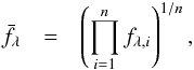 (A.1)where the product is over the individual spectra. We model each spectrum as a power law
 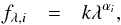 (A.2)and we get by inserting Eq. (A.2) into Eq. (A.1)
 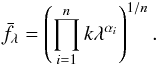 (A.3)We rewrite this expression and make the product a sum in the exponent
 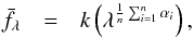 (A.4)where we see that the geometric mean of a sample of power laws is a power law,
  (A.5)with the mean index
  (A.6)
(A.6)
All Tables
All Figures
|
Fig. 1 Telluric correction for quasar SDSS1431+0535 where brown is the uncorrected spectrum and purple is the corrected spectrum and teal is the corrected spectrum smoothed by 50 pixels. The regions of pure noise are where the atmospheric transmission is ~zero, thus only leaving noise after correction. Residuals after correction are visible. The noise image is corrected correspondingly and regions severely affected are down-weighted in the weighted combination. |
| In the text | |
|
Fig. 2 Gaussian fit to [OIII]λ5007 for the object SDSS1354-0013. The red solid line is the linear least squared best fit. Gray dashed lines indicate the position of neighboring lines at the redshift of [OIII]. Only every 10th data point is shown for clarity. |
| In the text | |
|
Fig. 3 Quantile-quantile plot as a test for normality. An average over 100 pixels in the central regions where the continuum is assumed to be relatively flat is used. The inverse cumulative distribution for the sample is constructed and plotted against the corresponding quantiles for a normal distribution. The red line arises if we are sampling for a normal distribution. Since the points are slightly steeper, this indicates a more dispersed distribution. |
| In the text | |
|
Fig. 4 Top panel: composite spectrum with prominent emission lines marked. Upper middle panel: measure of intra-spectrum variability. The standard deviation of the constituent spectra as a function of wavelength, where to normalize the differing slopes between the different spectra, the fitted slope in each of the constituent spectra have been subtracted. Lower middle panel: signal-to-noise ratio. The composite spectrum is divided by the error spectrum, thus directly giving a measure of the signal strength. Bottom panel: number of contributing spectra as a function of wavelength. |
| In the text | |
|
Fig. 5 Dust extinction, AV, and redshift has been inferred for three HAQ quasars by fitting for the amount of reddening required to match the template with the observed spectrum. The black spectra are taken at the Nordic Optical Telescope (NOT) using the ALFOSC spectrograph. The black squares are optical ugriz photometric points from SDSS and UKIDSS YJHK bands. For varying amount of extinction at different redshifts, consistent results are found with previous usage of stitched composites. |
| In the text | |
|
Fig. 6 Quasar color, g−i, as a function of redshift, z. The full quasar sample from SDSS DR10 (Pâris et al. 2014) is shown in gray color. Bounding contours show the 0.5, 1, 1.5, 2σ contours of the density of points. The olive points are individual quasars from the SDSS sample which satisfy r< = 17. Overplotted in pink are the quasars contributing to the composite presented here. The quasar colors have been marginalized over in the right side where the tall pink lines are at the position of the composite quasars and the olive shaded area is the kernel density estimation of the distribution of quasars fulfilling the selection criteria. The gray-shaded area is the projection of the DR10 quasar sample. |
| In the text | |
|
Fig. 7 X-Shooter weighted arithmetic mean quasar composite on a linear wavelength scale in light brown. The positions of several prominent emission lines are marked. Overplotted in dark green is the corresponding composite generated from the full sample of SDSS quasars fulfilling the selection criteria and general agreement is observed, albeit with a brighter Balmer continuum in the SDSS-constructed composite. In purple is shown the results from fitting both a pure and a broken power law to the regions specified in Sect. 5 and they are observed to be indistinguishable. |
| In the text | |
|
Fig. 8 Comparison of different composites. The composites by Lusso et al. (2015), Vanden Berk et al. (2001), Telfer et al. (2002), Francis et al. (1991) are normalized to the X-Shooter composite at ~1450 Å and the composite by Glikman et al. (2006) is normalized to ours at ~3850 Å. Significant differences are visible blueward of Lyα due to differing IGM correction methods. Above 5000 Å significant host galaxy contamination is visible in the composite by Vanden Berk et al. (2001). Overplot in blue is a power law with slope αλ = −1.70 and normalized at ~1450 Å. |
| In the text | |
Current usage metrics show cumulative count of Article Views (full-text article views including HTML views, PDF and ePub downloads, according to the available data) and Abstracts Views on Vision4Press platform.
Data correspond to usage on the plateform after 2015. The current usage metrics is available 48-96 hours after online publication and is updated daily on week days.
Initial download of the metrics may take a while.