| Issue |
A&A
Volume 585, January 2016
|
|
|---|---|---|
| Article Number | A51 | |
| Number of page(s) | 13 | |
| Section | Extragalactic astronomy | |
| DOI | https://doi.org/10.1051/0004-6361/201527046 | |
| Published online | 16 December 2015 | |
An extreme [O III] emitter at z = 3.2: a low metallicity Lyman continuum source
1
INAF–Osservatorio Astronomico di Bologna, via Ranzani 1,
40127
Bologna,
Italy
e-mail:
This email address is being protected from spambots. You need JavaScript enabled to view it.
2
INAF–Osservatorio Astronomico di Roma, via Frascati
33, 00040
Monteporzio,
Italy
3
Departement of Physics and Astronomy, University of
California, Riverside, CA
92507,
USA
4
Harvard-Smithsonian Center for Astrophysics,
Cambridge, MA
02138,
USA
5
INAF–Osservatorio Astronomico di Trieste, via G. B. Tiepolo
11, 34131
Trieste,
Italy
6
Dipartimento di Fisica e Astronomia, Università degli Studi di
Bologna, Viale Berti Pichat
6/2, 40127
Bologna,
Italy
7
Observatoire de Genève, Université de Genève,
Ch. des Maillettes 51,
1290
Versoix,
Switzerland
8
Institute for Astronomy, 2680 Woodlawn Drive, Honolulu, HI
96822,
USA
9
Instituto de Astrofísica de Andalucía,
CSIC, Apartado de correos 3004,
18080
Granada,
Spain
10
Astronomy Department, University of Massachusetts,
Amherst, MA
01003,
USA
Received: 23 July 2015
Accepted: 22 September 2015
Abstract
Aims. Cosmic reionization is an important process occurring in the early epochs of the Universe. However, because of observational limitations due to the opacity of the intergalactic medium to Lyman continuum photons, the nature of ionizing sources is still not well constrained. While high-redshift star-forming galaxies are thought to be the main contributors to the ionizing background at z> 6, it is impossible to directly detect their ionizing emission. Therefore, looking at intermediate redshift analogues (z ~ 2−4) can provide useful hints about cosmic reionization.
Methods. We investigate the physical properties of one of the best Lyman continuum emitter candidate at z = 3.212 found in the GOODS-S/CANDELS field with photometric coverage from the U to the MIPS 24 μm band and VIMOS/VLT and MOSFIRE/Keck spectroscopy. These observations allow us to derive physical properties such as stellar mass, star formation rate, age of the stellar population, dust attenuation, metallicity, and ionization parameter, and to determine how these parameters are related to the Lyman continuum emission.
Results. Investigation of the UV spectrum confirms a direct spectroscopic detection of the Lyman continuum emission with S/N> 5. Non-zero Lyα flux at the systemic redshift and high Lyman-α escape fraction (fesc(Lyα) ≥ 0.78) suggest a low H i column density. The weak C and Si low-ionization absorption lines are also consistent with a low covering fraction along the line of sight. The subsolar abundances are consistent with a young and extreme starburst. The [O iii]λλ4959,5007+Hβ equivalent width (EW) is one of the largest reported for a galaxy at z> 3 (EW( [ O iii ] λλ4959,5007 + Hβ) ≃ 1600 Å, rest-frame; 6700 Å observed-frame) and the near-infrared spectrum shows that this is mainly due to an extremely strong [O iii] emission. The large observed [O iii]/[O ii] ratio (>10) and high ionization parameter are consistent with prediction from photoionization models in the case of a density-bounded nebula scenario. Furthermore, the EW([O iii]λλ4959,5007+Hβ) is comparable to recent measurements reported at z ~ 7−9, in the reionization epoch. We also investigate the possibility of an AGN contribution to explain the ionizing emission but most of the AGN identification diagnostics suggest that stellar emission dominates instead.
Conclusions. This source is currently the first high-z example of a Lyman continuum emitter exhibiting indirect and direct evidences of a Lyman continuum leakage and having physical properties consistent with theoretical expectation from Lyman continuum emission from a density-bounded nebula. A low H i column density, low covering fraction, compact star formation activity, and a possible interaction/merging of two systems may contribute to the Lyman continuum photon leakage.
Key words: galaxies: high-redshift / galaxies: evolution / galaxies: ISM / galaxies: starburst
© ESO, 2015
1. Introduction
One of the most pressing, unanswered questions in cosmology and galaxy evolution is determining which sources are responsible for the reionization of the intergalactic medium (IGM; Robertson et al. 2015) and are capable of keeping it ionized afterwards (Fontanot et al. 2014; Giallongo et al. 2015). Until recently, it was difficult to draw a consistent picture based on the different observational constraints (e.g., reconciling the ionizing background and the galaxy UV luminosity density; Bouwens et al. 2015). However, there are still many unconstrained parameters at z> 6, the most important one probably being the Lyman continuum escape fraction (fesc(LyC); Zackrisson et al. 2013). Unfortunately, it is not possible to directly detect Lyman continuum emission at the epoch of reionization or even in the aftermath (e.g., at any redshift z> 4.5), owing to the very high cosmic opacity (e.g., Worseck et al. 2014).
A number of surveys at 1 <z< 3.5 from the ground and with the Hubble Space Telescope (HST), have looked for ionizing photons by means of imaging or spectroscopy and there have been some claims of detections (Steidel et al. 2001; Shapley et al. 2006; Nestor et al. 2013; Mostardi et al. 2013, 2015). However, careful analysis of some claims combining different instruments (e.g., near-infrared spectroscopy and high spatial resolution probing LyC, Siana et al. 2015) shows that the individual detections must be considered with caution because of the difficulty in eliminating a possible foreground contamination (Vanzella et al. 2010b; Mostardi et al. 2015). Several other surveys reported only upper limits (Siana et al. 2010; Bridge et al. 2010; Malkan et al. 2003; Vanzella et al. 2010b, 2012; Boutsia et al. 2011; Grazian et al. 2015). This could be due to the rarity of relatively bright ionizing sources, as a consequence of the combination of view-angle effects (Cen & Kimm 2015), stochastic intergalactic opacity (Inoue & Iwata 2008; Inoue et al. 2014) and possibly intrinsically low escaping ionizing radiation on average, in the luminosity regime explored so far (L> 0.1 L∗, e.g., Vanzella et al. 2010b).
At higher redshifts, the galaxy contribution to the cosmic ionization budget must be inferred from other properties that correlate with their ability to contribute to ionizing radiation, if such properties exist. This is an open line of research with ground- and space-based facilities. Indirect signatures in the non-ionizing domain have been investigated by performing photoionization and radiative transfer modeling. Low column density and the covering fraction of neutral gas (which regulate the escape fraction of ionizing radiation) are related to a series of possible indicators:
-
the nebular conditions, (i.e., density-bounded or radiation bounded) traced by peculiar line ratios like large [O iii]/[O ii] ratios (e.g., Jaskot & Oey 2014; Nakajima & Ouchi 2014) or a deficit of Balmer emission lines given the inferred star formation rate (SFR) and the UV β slope (Fλ ∝ λβ; Zackrisson et al. 2013);
-
the strength of interstellar absorption lines as a tracer of neutral gas covering fraction (Jones et al. 2012; Heckman et al. 2011);
-
the structure of the Lyα emission line, its width, and its position relative to the systemic redshift (e.g., Verhamme et al. 2015);
-
the morphology and spatial distribution of the star formation activity (e.g., nucleation) which seems to be another property that favors efficient feedback and possibly a transparent medium for ionizing radiation (e.g., Heckman et al. 2011; Borthakur et al. 2014).
While all these features are promising signatures, possibly usable at the redshifts of the reionization, still missing is a direct link between them and the Lyman continuum emission. In this respect there is an ongoing effort to investigate this possible link in a particular class of sources that seems to possess all the above properties. The idea is to look for green pea (GP) galaxies in the nearby Universe. Green peas were discovered in the Galaxy Zoo project (Cardamone et al. 2009). They are small compact galaxies in the SDSS survey at 0.11 <z< 0.36, dominated by strong [O iii]λλ4959,5007 emission (EW( [ O iii ] λλ4959,5007) > 100 Å, up to ~1000 Å). This strong emission is thought to be related to a non-zero ionizing photon escape fraction (e.g., Jaskot & Oey 2014; Nakajima & Ouchi 2014). The typical physical properties of GPs are a low stellar mass (~108.5M⊙<M⋆< 1010.5M⊙), low metallicity (12 + log (O / H) = 8.05 ± 0.14, Amorín et al. 2010, 2012), high sSFR (sSFR = SFR/stellar mass, 1 to 10 Gyr-1, Cardamone et al. 2009), young age (a few Myr), showing Wolf-Rayet signatures (e.g., bumps and He ii ] λ4686 emission line), and extremely large Hα and [O iii]λ5007 equivalent widths. Their strong Lyα emission has recently been observed (Henry et al. 2015); however, no direct LyC signatures have currently been identified in green pea galaxies and the work is still continuing.
Similarly, it would be desirable to find Lyman continuum emitters at even higher redshift, within the first 2 Gyr after the Big Bang (z> 3) and to look for properties and physical mechanisms that allow ionizing photons to escape. Amorín et al. (2014a) report the properties of a z = 3.417 galaxy with possible indirect signature of ionizing photon leakage such as a large [O iii]/[O ii] ratio, but only an upper limit on the Lyman continuum emission. Very recently a class of candidate of strong Hβ+[O iii] emitters has been identified at much higher redshift (z> 6.5) by looking at the Spitzer/IRAC excess in channel 1 or 2 (depending on redshift; Schaerer & de Barros 2010; Ono et al. 2012; Labbé et al. 2013; Smit et al. 2014, 2015; Roberts-Borsani et al. 2015). The redshifts of two of the emitters have been spectroscopically confirmed at z = 7.73 and 8.67 with a combined equivalent width EW(Hβ + [ O iii ] ) ≃ 720 Å and >1000 Å (rest-frame), respectively (Oesch et al. 2015; Roberts-Borsani et al. 2015; Zitrin et al. 2015).
The nature of these objects is not well understood and further investigation is needed, though this will have to wait for the James Webb Space Telescope and extremely large telescopes.
We have identified two Lyman continuum leakers in Vanzella et al. (2015; hereafter V15): Ion1 and Ion2. These galaxies were selected as Lyman continuum emitters through a photometric selection that is based on the comparison between the observed photometric fluxes and colors probing the Lyman continuum emission and predictions from the combination of spectral synthesis models (e.g., Bruzual & Charlot 2003) and intergalactic medium (IGM) transmissions (Inoue et al. 2014).
In this work we present the source with one of the largest [O iii]λλ4959,5007 line equivalent widths currently known (EW ~ 1500 Å, rest-frame) at z> 3 and with a plausible leakage of ionizing radiation. Ultraviolet (VLT/VIMOS), optical, and near-infrared (Keck/MOSFIRE) rest-frame spectroscopy are presented, as well as a detailed multifrequency analysis with the aim of testing the aforementioned signatures of linking Lyman continuum. We also use the extreme line ratios to investigate the nebular conditions. To this end we also compare the observed Ion2 properties with theoretical predictions from photoionization models.
Ion2 shares some of the properties of sources recently identified at much higher redshift (in particular the large EW (Hβ+ [O iii]) and is therefore relevant to reionization, with the advantage of anticipating the rest-frame optical spectroscopic investigation of such extreme objects.
The paper is structured as follows. The spectroscopic and photometric data are described in Sect. 2. In Sect. 3, we present the physical properties derived from the reanalyzed UV spectrum and the newly acquired near-infrared MOSFIRE spectrum, and alongside we present the properties derived from the photometry. We also review previously reported properties (V15) in the light of the new data. In Sect. 4, we discuss a possible active galactic nucleus (AGN) contribution to the observed Ion2 spectra. We summarize our main conclusions in Sect. 5.
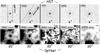 |
Fig. 1 Postage stamps of Ion2 in B435, V606, i775, z850, H160, IRAC 3.5 μm, IRAC 4.5 μm, IRAC 5.8 μm, IRAC 8.0 μm, and MIPS 24 μm. The sizes of the images are 4′′ × 4′′ for the HST bands and 20′′ × 20′′ for the Spitzer bands. |
We adopt a Λ-CDM cosmological model with H0 = 70 km s-1 Mpc-1, Ωm = 0.3, and ΩΛ = 0.7. We assume a Salpeter IMF (Salpeter 1955). All magnitudes are expressed in the AB system (Oke & Gunn 1983).
2. Data
2.1. Spectroscopy
The available low-resolution (LR, R = 180) and medium-resolution (MR, R = 580) VLT/VIMOS spectroscopy covering the spectral ranges 3400–7000 Å and 4800–10 000 Å were obtained during 2005, with 4hr exposure time for both LR and MR spectra. The LR spectrum continuum sensitivity is S/N ~ 0.8 at 3700 Å with 4 h and m(AB) = 26.5 assuming seeing 0.8′′ and airmass 1.2. It is calculated over one pixel along dispersion and 2 × FWHM (full width half maximum) along spatial direction. (Popesso et al. 2009; Balestra et al. 2010). Slit widths of 1′′ were adopted and the median seeing during observations was 0.8′′. We have newly reduced both configurations, in particular focusing on the Lyman continuum emission (LR-spectrum) and the ultraviolet spectral properties in the non-ionizing domain (MR-spectrum). Reduction was done in two ways: as described in Balestra et al. (2010) and the AB–BA method as described in Vanzella et al. (2011, 2014b). Both methods produce consistent results.
Recently, a near infrared spectrum of Ion2 was obtained with Keck/MOSFIRE in March 2015 (PI: Günther Hasinger). Integration time of 32, 32, and 36 min were obtained in the J-, H-, and K-bands, respectively, with the AB–BA dithering pattern of 2.9′′. The adopted slit width was 0.7′′ producing a dispersion of 1.30 Å, 1.63 Å, and 2.17 Å per pixel, in the J-, H-, and K-bands, respectively; the pixels scale along the spatial direction was 0.18′′/pixel. Ion2 was inserted in a mask aimed to target low-z objects as well. The J-band is useful for monitoring low-z emission lines.
Reduction was performed using the standard pipeline1. Briefly, two-dimensional sky-subtracted spectra, rectified and wavelength calibrated, are produced from which the one-dimensional variance weighted spectrum is extracted with a top-hat aperture. The wavelength solution was computed from sky emission lines (e.g., Rousselot et al. 2000) in the three bands reaching an rms accuracy better than 1/20, 1/30, and 1/40 of the pixel size in J-, H-, and K-bands, respectively (typical rms <0.05 Å).
Emission line properties.
Flux calibration was performed by observing the standard star A0V HIP 26577. Given the slit width (0.7′′) and the median seeing conditions during observations (0.85′′), particular care must be devoted to slit losses. For this reason we checked it by using a star included in the same science mask (WISE 895) for which the continuum is very well detected in the entire MOSFIRE wavelength range, and whose J-, H-, and K-band total magnitudes are known from CANDELS (Grogin et al. 2011; Koekemoer et al. 2011) and HUGS photometry (Fontana et al. 2014) with typical S/N> 40. From the star WISE 895 and its near infrared photometry we derive a correction factor for slit losses and possible centering effects of about 50%. With this correction the total line flux (Hβ+[O iii]λλ4959,5007) derived from the MOSFIRE spectrum is fully consistent with the total line flux derived from the SED fit and K-band excess (see Sect. 3.3). Ion2 is composed of two blobs separated by 0.2′′ (see Fig. 12) each one with a half-light radius Re ≃ 0.3 kpc, or less than 0.1′′ at z = 3.212. Therefore, the slit losses for the entire system at the 0.7′′ MOSFIRE entrance slit are modulated primarily by the seeing during observations, which was on average 0.85′′. A correction factor of 1.4 is consistent with the expected fraction of light falling outside the slit for a perfect centering of the target and Gaussian seeing with FWHM = 0.85′′. The correction is also compatible with the discussion in Steidel et al. (2014). Therefore, a correction factor of 1.5 is reasonable in our configuration and observational conditions and include a possible small centering uncertainty.
Line fluxes, errors, and limits from VIMOS and MOSFIRE spectra are given in Table 1.
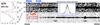 |
Fig. 2 Two-dimensional LR VIMOS UV spectrum of Ion2 with different cuts to emphasize the spectral features Lyα and Lyβ (bottom) and the Lyman continuum λ< 912 Å, in the range 855–910 Å (top, vertical dotted blue lines). On the left, we show the moving average calculated within a rectangular aperture (855−910 Å × 1.25′′, red-dotted rectangle) in the spatial direction divided by its rms on the left side. A signal is detected at λ< 912 Å with S/N> 5. The inset shows the pixel distribution of the background after sky-subtraction in the region 855–910 Å (derived from the S/N spectrum). The distribution is symmetric (skewness = −0.016) with the mean and median close to zero, +0.0057 and −0.014, respectively. No significant systematic effects are present. |
2.2. Photometry
Deep U-band imaging was performed with the VLT/VIMOS instrument providing a 1σ depth of mag ~30 within 1 circular aperture. We refer the reader to Nonino et al. (2009) for a complete description of the data reduction (see also Vanzella et al. 2010a).
The photometry from the U VIMOS band to the Spizter/IRAC 8.0 μm band is taken from the CANDELS GOODS-S multiwavelength catalog (Guo et al. 2013). The optical Hubble Space Telescope images from the Advanced Camera for Surveys (ACS) combine the data from Giavalisco et al. (2004), Beckwith et al. (2006) and Koekemoer et al. (2011). The field was observed in the F435W, F606W, F775W, F814W and F850LP bands. Near-infrared WFC3/IR data combines data from Grogin et al. (2011), Koekemoer et al. (2011) and Windhorst et al. (2011) with observations made in the F098M, F125W, and F160W bands. The VLT/HAWK-I Ks-band imaging are taken from the HUGS survey (Fontana et al. 2014). The Spitzer/IRAC 1 and 2 data are taken from the SCANDELS survey (Ashby et al. 2015), while the IRAC 3 and 4 data are taken from Ashby et al. (2013). Hereafter, we will refer to the filters F435W, F606W, F775W, F814W, F850LP, F098M, F125W, and F160W as B435, V606, i775, I814, z850, Y098, J125, and H160, respectively.
We also checked detection in the Spitzer/MIPS bands and in the Herschel data. As shown in Fig. 1, we are able to put an upper limit to the MIPS 24 μm flux (S/N< 2, mAB = 22.27 ± 0.90, Santini et al. 2009), while it is undetected in Herschel bands (<1.2 mJy, <1.2 mJy, <2.4 mJy in the 70 μm, 100 μm, and 160 μm bands, respectively, 5σ upper limits).
3. Physical properties
3.1. Spectroscopic detection and spatial distribution of the Lyman continuum emission
Spectroscopic detection of stellar Lyman continuum emission at z ~ 3 has been previously claimed for few galaxies (e.g., Steidel et al. 2001; Shapley et al. 2006) but this kind of detection is a difficult task, mainly because of foreground contamination (Vanzella et al. 2010b; Siana et al. 2015; Mostardi et al. 2015), and a clear spectroscopic detection of Lyman continuum emission at high redshift is still missing. The only two spectroscopic detections reported in the literature are from Steidel et al. (2001) in a stack of 29 LBGs (Lyman break galaxies) and individually in a subsequent spectroscopic follow-up in 2 out of 14 LBGs observed by Shapley et al. (2006), dubbed D3 and C49. Vanzella et al. (2010b) performed dedicated simulations to derive the probability of foreground contamination, specifically for the observational setups adopted by Steidel et al. (2001) and Shapley et al. (2006). In both cases, the probability was high enough to raise doubts about their reliability. Subsequently, the two sources with the possible LyC detection of Shapley et al. (2006) were not confirmed as LyC sources. In particular D3 was ruled out by much deeper narrow-band imaging by Iwata et al. (2009) and Nestor et al. (2011), and C49 was excluded from the list of LyC sources after the possible spectroscopic confirmation of a close foreground lower redshift source (Nestor et al. 2013) and finally confirmed to be a z = 2.029 foreground source (Siana et al. 2015). Therefore, at present there are no direct LyC detections from star-forming galaxies, apart from the source reported in the present work.
The VIMOS LR spectrum of Ion2 shows a clear signal detected blueward of the Lyman limit. We performed a careful reanalysis of the Ion2 low-resolution UV spectrum by computing the moving average of the flux at λ< 910 Å and we find a signal with S/N> 5 (Fig. 2). While several systematics can affect the derivation of the LyC signal (e.g., background substraction, Shapley et al. 2006), we use different methods of sky subtraction (the ABBA method and polynomial fitting with different orders) and they all provide consistent results. In particular the same moving average in the LyC region calculated over the S/N two-dimensional spectrum we derived with ABBA method (see Vanzella et al. 2014a) produces stable results with no significant systematics and a signal (>5σ) at the same spatial position of the target. This signal can be interpreted as a direct detection of the Lyman continuum emission, but the presence of the two components in the HST images can cast some doubts on the origin of this detection. However, assuming that the faintest component keeps the same magnitude as the derived B435 magnitude (27.25 ± 0.24; V15) at shorter wavelengths, the average S/N in the range 3600–3840 Å is ~0.5 per pixel (from ETC). Averaging over 20 pixels (as we did in Fig. 2) we would expect S/N ~ 2.2. In addition, the B-band dropout signature of such a component (B − V = 0.62, V15) between the B435 and V606 prevents a possible increased emission approaching the U-band, unless an emission feature is boosting the U-band magnitude. In this case the only possible line would be [O ii]λ3727 which would also imply a certain amount of star formation activity, which in turn would be detectable through Balmer and/or oxygen lines in the wide spectral range probed here. The most likely explanation is that the spectroscopic detection is due to a Lyman continuum emission emerging from the brightest Ion2 component. Furthermore, the ground-based VLT/VIMOS U-band spatial distribution shows that most of the U-band flux is emitted from the brightest component (Fig. 3).
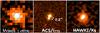 |
Fig. 3 Ground-based VLT/VIMOS U-band observation of Ion2 at a resolution of 0.2′′/pixel (left panel). The contour of the system (derived from the ACS/i775 band, center panel) is indicated and superimposed in blue onto the VIMOS U-image and onto the HAWK-I Ks image (right panel). The cutouts are 2.6′′ × 2.6′′. |
However, the U-band probes both ionizing and non-ionizing photons (λ< 937 Å), so a fraction of the signal is not only due to Lyman continuum photons, and the ground-based observations are clearly limited in terms of resolution, as seen in Fig. 3.
The only way to clarify the exact position and the detailed spatial distribution of the Lyman continuum emission is to perform dedicated HST observations. A proposal to observe Ion2 with HST/F336W (17 orbits) has recently been approved (PI: Vanzella, cycle 23). Hopefully, emission line diagnostics can be used to characterize the gaseous and stellar content of Ion2 and will provide some hints about a Lyman continuum leakage, as discussed in the next section.
From the signal detected at 880−910 Å, we derive the relative fesc(LyC) defined as: 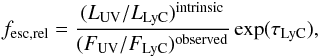 (1)where (LUV/LLyC)intrinsic is the intrinsic UV to ionizing luminosity density, (FUV/FLyC)observed is the observed UV to ionizing flux density, and exp(τLyC) is the LyC attenuation due to the IGM. The signal measured in the LR spectum corresponds to ~26.95 AB magnitude and m1500 = 24.60 is the magnitude observed at 1500 Å rest-frame (using the V606 band corrected for the Lyα flux). The average IGM transmission is 0.54 in the 880−910 Å range (Inoue & Iwata 2008; Inoue et al. 2014) and assuming L1500/L900 = 3 (Nestor et al. 2013), we get:
  (2)If we relax the assumption about the intrinsic L1500/L900 ratio, then fesc,rel increases. Or conversely, assuming the maximum IGM transmission at z = 3.2 (0.74), L1500/L900 must be lower than 6.5 to keep fesc,rel< 1.
3.2. Physical properties of the interstellar medium
As described in Sect. 2, we use VLT/VIMOS and Keck/MOSFIRE spectroscopy to obtain a wide Ion2 spectral coverage with 850 <λ< 5700 Å (rest-frame). The emission line fluxes, FWHMs, and equivalent widths are summarized in Table 1. Several lines are barely detected with signal-to-noise <3 (e.g., Hβ). However, thanks to the well constrained redshift (see below) and because we know the exact wavelength positions of some features, we do not expect strong systematics. This is the case for the Hβ and [O ii]λ3727 lines, whose signatures are indeed at the expected positions.
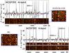 |
Fig. 4 Two- and one-dimensional near-infrared spectra of Ion2 in the MOSFIRE H- and K-band. Two insets show the regions where Hβ and the [O ii]λ3727 doublet are expected from the redshift. The gray stripes in the one-dimensional spectra indicate the position of the sky lines. |
Individual line flux errors were derived using the error spectrum. Additionally, we performed simple simulations to test the error associated with emission line ratios in the MOSFIRE spectrum (Fig. 4). Figure 5 shows the positions where the [O iii]λ5007 observed line has been added to the sky-subtracted spectrum (labeled with numbers from 1 to 10) with different dimming factors (DIM = 1, 3, 10 from top to bottom). This provides a rough estimate of the typical error and S/N ratio of our measurements. For example, the typical error associated with the line ratio is [ O iii ] λ5007 / [ O iii ] λ4959 = 4.1 ± 0.7, which is consistent with the theoretical ratio (2.99) within 1.4σ (if necessary, we fix the ratio to the theoretical value). Furthermore, the [O iii]λ5007 line dimmed by a factor of 10 (bottom panel in Fig. 5) is similar to the observed Hβ 2D spectrum, indicating a likely [O iii]λ5007 to Hβ ratio ≥10. The marginal Hβ detection (with S/N ~ 2) allows us to derive a ratio [ O iii ] / Hβ = 14.7 ± 5.1, while for the [O ii] line the non-detection translates to a 2σ lower limit of [ O iii ] λ5007 / [ O ii ] λ3727 > 10 (uncorrected for dust in both cases). The errors derived with our simulations are fully consistent with those derived from the error spectrum.
The first property derived from emission lines is the spectroscopic redshift. As already reported in V15, the C iii ] λ1906.68−1908.68 transition is clearly detected in the VIMOS MR spectrum (with S/N = 8, Fig. 6). This feature shows a symmetric shape with a relatively large FWHM (=400 km s-1) with respect to other lines like Lyα and [O iii], suggesting that the two components have similar intensities even if they are blended and not resolved. The redshift we derive from C iii ] is fully consistent with the redshift of oxygen lines 4959–5007 Å identified in the MOSFIRE spectrum (see Table 1). This provides a robust estimate of the systemic redshift, z = 3.2127 ± 0.0008.
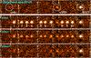 |
Fig. 5 Observed and simulated two-dimensional MOSFIRE spectrum, with the observed [O iii]λ5007 line replicated at different wavelength positions with different dimming factors (DIM). See text. |
We derived the ionization parameter and the oxygen and carbon abundances using a modified version of the HII-CHI-mistry code (Pérez-Montero 2014), adapted to provide metallicity, C/O, and ionization parameter in a Te-consistent framework, based on the comparison of the observed UV and optical nebular lines with a grid of cloudy photoionization models (Ferland et al. 2013). The lines used as input are C ivλ1550, C iii]λ1909, O iii]λ1666, and Hβ, while the C ivλ1550/C iii]λ1909 (sensitive to the ionization parameter), C iii]λ1909/O iii]λ1666 (proportional to C/O), [O iii]λ5007/O iii]λ1666 (sensitive to the electron temperature) and (C ivλ1550+C iii]λ1909)/Hβ ratios are compared with model-based ratios in a χ2-weighted minimization scheme. The derived abundances and the ionization parameter are 12 + log (O / H) = 8.07 ± 0.44, log (C / O) = −0.80 ± 0.13, and log U = −2.25 ± 0.81. We also derive these quantities using all the lines except O iii]λ1666 (S/N ~ 1.7) and we obtain 12 + log (O / H) = 7.79 ± 0.35 and log U = −2.32 ± 0.11 (C/O can not be derived without O iii]λ1666). Both sets of lines lead to low metallicity and a high ionization parameter (in the following, we consider the results obtained with all the line measurements and upper limits). Ion2 metallicity is similar to the typical green pea metallicity (12 + log (O / H) = 8.05 ± 0.14, Amorín et al. 2010). The metallicity and the ionization parameter are also consistent with extreme emission-line galaxies up to z ~ 3.5 (Amorín et al. 2014b,a, 2015). The metallicity of Ion2 is also consistent with the mean metallicity of star-forming galaxies selected through their extreme EW([O iii]) (Maseda et al. 2014; Amorín et al. 2015; Ly et al. 2014). Moreover, the Ion2 C/O ratio is strongly subsolar (C / O⊙ = −0.26Asplund et al. 2009) and is consistent with the trend in C/O vs. O/H for local galaxies (Garnett et al. 1999), which shows a nearly linear increase in C/O with Z> ~0.2 Z⊙. The low O/H and C/O abundances of Ion2 are similar to those found in other strong emission-line galaxies at z ~ 1−3 (e.g., Christensen et al. 2012; Stark et al. 2014; James et al. 2014) and suggest a significant contribution of O and C produced by massive stars, which is also consistent with very young and extreme starbursts.
We compare the metallicity and the ionization parameter with the results presented in Nakajima & Ouchi (2014) in Fig. 7. Overall, Ion2 has a lower metallicity than all other galaxy populations presented in their work and one of the highest ionization parameters. The higher ionization parameter is in line with a possible Lyman continuum leakage that could be explained with a low neutral hydrogen column density. Also, the Ion2 extreme [O iii]λ5007/[O ii] ratio, the metallicity, and the ionization parameter are consistent with cloudy models with a non-zero Lyman continuum escape fraction (Nakajima & Ouchi 2014,Fig. 11)
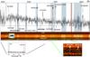 |
Fig. 6 1D and 2D UV VLT/VIMOS MR spectra. The transparent blue stripes indicate the positions of the emission sky lines. The transparent red stripes indicate the telluric molecular sky absorptions bands, B- and A-bands at ~6900 Å and ~7600 Å. In the same panel, three 2D spectra are shown, the reduced, rms and signal-to-noise ratio, from bottom to top. The inset on the left side shows the double-peaked Lya line (from V15). In the bottom right a zoom-in around the He iiλ1640 and O iii]λ1666 positions is shown. Their detections remain tentative. In the bottom left, the 1D spectrum shows the relative Lyα flux in comparison with other lines. |
The identification of Lyman continuum leakage from green pea galaxies is a continuing line of research (e.g., Jaskot & Oey 2014; Nakajima & Ouchi 2014; Borthakur et al. 2014; Yang et al. 2015) and the green pea nature of Ion2 and its LyC leakage represent the first concrete attempt to link these two properties. Ion2 represents an extreme case of green pea galaxy; it is the highest redshift (z> 3), ultra-strong oxygen emitter (with EW( [ O iii ] λλ4959,5007) ~ 1100 Å) currently known. The Lyman continuum leakage observed in Ion2 allows us to investigate the relationship between the LyC leakage and physical and morphological properties. However, as shown in Stasińska et al. (2015), the [O iii]/[O ii] ratio is also related to the specific star formation rate and the metallicity: the [O iii]/[O ii] ratio increases with increasing sSFR and decreasing metallicity. For Ion2, the observed ratio is ≥15 making Ion2 an outlier in the oxygen abundance vs. the [O iii]/[O ii] ratio relation and the EW(Hβ) (i.e., sSFR) vs. the [O iii]/[O ii] ratio (Fig. 2, Stasińska et al. 2015); the Ion2 ratio is higher by ~0.6 dex for the observed EW(Hβ) (Table 1) and the ratio is higher by ~1 dex than galaxies in the SDSS sample with similar metallicities. The Ion2 [O iii]/[O ii] ratio is also higher than expected for the derived stellar mass, SFR, and sSFR (Nakajima & Ouchi 2014). Therefore, we conclude that the extreme [O iii]/[O ii] ratio is due to unusual physical conditions (density-bounded nebula), which imply a low column density of neutral gas, and so favor leakage of ionizing photons (Nakajima & Ouchi 2014).
3.3. Physical properties derived from the photometry
While the emission lines highlight Ion2 ISM physical properties, we also use the photometry to confirm findings such as the large [O iii] emission and derive other physical parameters. From Fig. 8, the jump in the K-band is evident, K = 22.97 ± 0.02 while the continuum level in the adjacent bands, H160, and IRAC Channel 1 is ≃24.15. The Δm ≃ 1.1 magnitude in the HAWKI K-band corresponds to an additional flux of 3.1 × 10⁻¹⁶ erg/s/cm2, which corresponds to an observed equivalent width of 6700 Å (1600 Å rest-frame). The total flux derived for Hβ+[O iii]λλ4959,5007 from the MOSFIRE spectrum (see Table 1) is fully compatible with the flux estimated from the K-band excess (after correcting for slit losses for the three lines, see above). The derived Hβ + [OIII] equivalent width is one of the largest ever observed at z> 2. The measured line ratios among the Hβ+ [O iii]λλ4959,5007 suggest the [O iii]λ5007 rest-frame equivalent width is ≃1100 Å, with a similar value to the few extreme cases reported in the literature at z ~ 1−2 (Atek et al. 2011; Amorín et al. 2014b; Maseda et al. 2014). The [O iii]/Hβ ratio is also higher than the value reported in Holden et al. (2014) for LBGs at z ~ 3.5, while the ratio is higher in this sample than in the local Universe (Brinchmann et al. 2004). At z> 6 large equivalent widths of Hβ+[O iii] have also been reported, measured through photometric excess detected in the Spitzer/IRAC channels (e.g., Finkelstein et al. 2013; Smit et al. 2014; Oesch et al. 2015). While these cases can be spectroscopically investigated only with future facilities, such as the James Webb Space Telescope (JWST) and Extremely Large Telescope class, in our case the MOSFIRE near-infrared spectroscopy has allowed us to access the details of the lines.
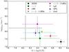 |
Fig. 7 Comparison of the metallicity and ionization parameter (U = q/c) between the mean sample properties from Nakajima & Ouchi (2014) and Ion2 with 1σ uncertainties. Ion2 is compared to local galaxies from the SDSS survey, a galaxy sample at z ~ 1, a Lyman break galaxy (LBG) sample at z ~ 2.5, a Lyman alpha emitter (LAE) sample at z ~ 2.5, local Lyman break analogues (LBAs), LyC emitters, and Green Peas (GPs). See Nakajima & Ouchi (2014) and references therein for a complete description of these samples. |
We derive the SFR from the UV luminosity, Hβ, and Lyα lines (Kennicutt 1998), neglecting dust attenuation (see Appendix B). We get SFR(UV) = 15.6 ± 1.5 M⊙yr-1, 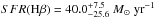 , and SFR(Lyα) = 14.3 ± 1.0 M⊙yr-1. The three SFR indicators are consistent within 68% confidence levels, while SFR(Hβ) is higher than the other two. The resonant nature of Lyα photons prevents us from deriving the SFR precisely with this line (e.g., Atek et al. 2014). On the other hand, the Hβ line is barely detected (Table 1). The higher SFR derived from the Hβ line can be explained if the age of the galaxy is significantly younger than 100 Myr because of the different equilibrium timescales between UV and nebular emission lines. However, this is not the case according to the SED fitting, with an age for Ion2~200 Myr. By comparing SFR(UV) and SFR(Lyα), we derive a Lyman-α escape fraction fesc(Lyα) ≥ 0.78 (fesc(Lyα) ≥ 0.28 by using SFR(Hβ) instead of SFR(UV)). This high Lyα escape fraction can be related to a blue β slope (e.g., Hayes et al. 2014), but also to a low H i column density (NH i ≤ 1018 cm-2; Yang et al. 2015; Henry et al. 2015).
The Ion2 Lyα profile has been described in V15: it exhibits a blue asymmetric tail. A low column density would be consistent with the bluer Lyα emission at the systemic redshift, and also with the high ionization parameter, and so with a leakage of ionizing photons. The star formation activity confined in a small physical volume can also favor the escape of ionizing radiation (e.g., Heckman et al. 2011; Borthakur et al. 2014). Furthermore, detailed analysis of the local blue compact dwarf galaxy NGC 1705 shows that O stars are able to photoionize volumes far from their location (Annibali et al. 2015), which could create density-bounded conditions. Moreover, the spatial density of O stars in NGC 1705 increases toward the center of the galaxy, forming a sort of super star cluster efficient at ionizing its environment. Ion2 could display a similar condition, being spatially resolved but nucleated in the ultraviolet (1400 Å), in which a young super star cluster could be present in the core and significantly contributing (or totally contributing if the AGN is absent) to the ionization field. Interestingly, because Ion2 has two components likely at a similar redshift (Sect. 3.4), the leakage of ionizing photons can also be favored by the merging/interaction of these two components (Rauch et al. 2011).
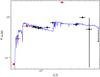 |
Fig. 8 Observed Ion2 SED (black and red dots). We show the best SED fit in blue and the integrated fluxes with blue crosses. We exclude photometric points (in red) affected by the IGM and strong emission lines (Lyα, [O iii]) from the SED fitting. The arrow indicates the 1σ upper limit. |
From SED fitting, we also derive a stellar mass log (M⋆/M⊙) = 9.5 ± 0.2 and an age of the stellar population (since the onset of the star formation) log (Age / yr) = 8.6 ± 0.2. We notice that while the two Ion2 components are separated in the BViz-bands, they are seen as a unique galaxy in the other bands, and the stellar mass is the total stellar mass of the two components. Given the very close separation between the two (0.2′′), we decided to avoid any tentative decomposition and SED fitting of each component individually, especially in the Spitzer/IRAC bands where the pixel size is 1.22′′ and the decomposition is in practice not possible. Using SED fitting and anchoring the best fit to the β slope derived from UV spectrum fitting (Appendix B), we predict the expected observed L(IR)24μm assuming energy balance (i.e., a balance between the energy absorbed in the UV/optical – we integrate over 912 Å to 3 μm – and re-radiated in the IR). The MIPS 24 μm observations probe the PAH feature at 6.2 μm (rest-frame), which can be used to derive the total IR luminosity (i.e., IR luminosity integrated over 8–1000 μm) and then the bolometric SFR (Pope et al. 2008; Rujopakarn et al. 2012). Because the SFR derivation relies on several assumption (star formation history, age, metallicity, IMF, Kennicutt 1998), we rely on the comparison between predicted L(IR)SED and derived L(IR)24μm, rather than relying on a SFR comparison. From the MIPS 24 μm upper limit, we derive 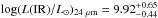 , while from SED fitting we derive
 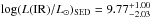 . The SED predicted and observed L(IR) are consistent, but the uncertainties are too large to exclude an AGN contribution to the IR flux. A discussion of a possible AGN contribution is found in Sect. 4.
Ion2 also shows an excess in the IRAC2 band, in comparison with the IRAC1 channel. This excess cannot be explained by emission lines or other features from the two blobs (e.g., a contamination by a strong emission line as Hα would imply z> 5.0 for the emitting galaxy). While we do not have a satisfactory explanation, we note that the rest-frame wavelength interval probed by IRAC2 (9500–11 900 Å) cannot be explored in detail before the launch of JWST. Therefore that part of the spectrum is poorly known, especially for sources in the distant universe. In this work we do not comment further about this feature that, however, does not affect our results. We summarize the physical properties of Ion2 in Table 2.
Ion2 physical properties.
3.4. Properties previously reported: summary
Ion2 was reported as a Lyman continuum emitter candidate in V15. Here, we briefly summarize the Ion2 properties reported in this reference.
Ion2 is a compact source (300 ± 70 parsecs) with two visible components. The presence of these two blobs can be misleading when trying to assess the detection of a possible Lyman continuum emission, because multiple components are often the source of foreground contamination (Vanzella et al. 2010b; Siana et al. 2015; Mostardi et al. 2015). However, BViz magnitudes have been derived for each component after subtracting the close companion with a GALFIT fitting procedure (see V15). The two show the same break between the V606 and B435 bands and the absence of any spurious (low-z) emission line along the wide wavelength range probed here (from 3400 Å up to 24 000 Å) support that the faint component is a physical companion of the brightest one (i.e., at z = 3.2). Furthermore, the slit orientation in the MOSFIRE observation also maximizes the separation in the spatial direction (see Fig. 1), though the seeing FWHM is significantly larger than the separation. Therefore, based on photometric shape and spectroscopic arguments we conclude that the two components are at the same redshift.
Interestingly, the Lyα profile exhibits a double-peaked emission where the bluer component is half of the main red peak and has a redshift consistent with the systemic redshift (z = 3.212, Fig. 9). If the two Lyα components are due to the two Ion2 blobs, we would expect multiple-peaked [O iii] emissions (Kulas et al. 2012), which are not present in the Ion2 MOSFIRE spectrum (see Sect. 3.2). If the observed Lyα photons arise only from the brightest Ion2 component, as discussed above it can be consistent with a low neutral gas column density (e.g., Verhamme et al. 2015) and with the escape of Lyman continuum photons (Behrens et al. 2014). However, a small shift of the maximum of the profile compared to the systemic redshift is expected where there is Lyman continuum emission (i.e., log (NH i) < 18) with a maximum peak separation <300 km s-1 (Verhamme et al. 2015). However, the non-detection of low-ionization absorption lines (e.g., [C ii]λ1334, [Si ii]λ1260) is consistent with a low neutral hydrogen column density allowing the escape of ionizing photons and a low covering fraction along the line of sight (Heckman et al. 2011; Jones et al. 2012, 2013). We possibly detect O i + [ Si ii ] λ1303 with EW = −1.2 ± 0.7 Å and tentatively [ Si ii ] λ1526 with EW = −1.0 ± 0.7 Å. However, the signal-to-noise ratio is low (S/N ~ 2). Assuming a 1σ fluctuation, we can put a lower limit on the EW of non-detected lines as EW> −0.7 Å. This is in line with the results from Shapley et al. (2003) at z ~ 3: galaxies with high Lyα equivalent width exhibit much weaker low-ionization absorption lines than galaxies with low EW(Lyα).
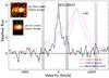 |
Fig. 9 Velocity profiles of [O iii]λ5007 and Lyα lines relative to systemic. The [O iii]λ5007 line is shown in black, the Lyα first order in red, and the Lyα second order with the dashed blue line. The positions and widths of the sky lines are indicated by gray stripes. |
Finally, Ion2 is not detected in the 6 Ms X-ray Chandra image (LX< 2−3 × 1042 erg s-1) and most of the high-ionization emission lines are not detected (e.g., N vλ1240, C ivλ1550). However, from the UV spectrum reanalysis, we report a tentative detection of He iiλ1640 (see Sect. 3.2): this line is barely detected in the ABBA spectrum, but not in the Balestra et al. (2010) spectrum. Furthermore, V15 also reported a possible variability of Ion2. We discuss the possibility of an AGN contribution in Sect. 4.
4. Is Ion2 an AGN?
We now discuss the possibility that the main source of UV ionizing photons is an AGN. First of all, the UV emission is resolved so it is most probably due to the stellar population, not to an AGN. Therefore, an AGN could contribute to the SED but it would not dominate it at all wavelengths.
Unfortunately, we cannot use the Baldwin, Phillips & Terlevich diagram (BPT, Baldwin et al. 1981) to discriminate between star formation and AGN, because Hα and [N ii] emission lines are out of the MOSFIRE wavelength range. Juneau et al. (2011) proposed an alternative to the BPT diagram, with the so-called MEx diagram based on the comparison between stellar mass and [O iii]λ5007/Hβ ratio. The probability that an object is an AGN associated with the MEx diagram is not defined at the Ion2 position (Juneau et al. 2014), although the large [O iii]λ5007-to-Hβ ratio would classify Ion2 as an AGN. Other diagnostic diagrams have been proposed, such as [O iii]λ5007/Hβ vs. [O ii]λ3727/Hβ (Lamareille et al. 2004). In this diagram, Ion2 would also be classified as an AGN because of the large [O iii]λ5007/Hβ ratio. However, for both diagnostics (MEx and [O iii]λ5007/Hβ vs. [O ii]λ3727/Hβ), there is no known AGN at a similar locus to Ion2. Alternatively, photoionization models predict a possible increase in [O iii]/[O ii] with decreasing metallicity and increasing ionization parameter (Nakajima & Ouchi 2014).
As already stated, Ion2 remains undetected even in the 6 Ms X-ray Chandra survey. According to the empirical relation between the [O iii]λ5007 luminosity and the X-ray luminosity (e.g., Panessa et al. 2006), given the extreme [O iii]λ5007 emission the expected X-ray luminosity would be LX ~ 1045 ergs-1 if the [O iii]λ5007 emission is associated with an AGN. Considering the scatter in the L( [ O iii ] λ5007)-LX relation, we can derive a lower limit of LX ≥ 5 × 1043 ergs-1, which would be easily detectable in the 6 Ms Chandra data (with typical S/N> 10), independently of the source position in the X-ray image. However, extremely obscured AGNs can have lower X-ray luminosity than expected from the L( [ O iii ] λ5007)-LX relation, this AGN possibly being Compton-thick AGNs (e.g., Vignali et al. 2010). The infrared and X-ray luminosities derived from the MIPS detection and the 6 Ms upper limit, respectively, can be compared with the properties of known obscured AGN (Lanzuisi et al. 2015): Ion2 properties can only be consistent with a faint and highly obscured AGN (e.g., Lutz et al. 2004).
The large EW([O iii]λ5007) is unusually large for all types of AGNs (Table 1, Caccianiga & Severgnini 2011), while such a large equivalent width has been already reported for some star-forming galaxies at lower redshift (e.g., Atek et al. 2011; van der Wel et al. 2011; Brammer et al. 2012).
The UV spectrum is quite unexplored as a diagnostic for AGN/star-forming galaxies classification, but the observed narrow lines (Table 1) exclude the presence of broad-line AGN. We also compare Ion2 emission line ratios with typical UV emission line ratios in narrow line AGN. Nagao et al. (2006) present the UV spectrum analysis of narrow-line QSOs and narrow-line radio galaxies at 1.2 ≤ z ≤ 3.8 (see also De Breuck et al. 2000). The first evidence against a possible AGN contribution to Ion2 spectra is the lack of C ivλ1550 detection. This line is detected in all AGN types studied in Nagao et al. (2006). The typical line ratio C iii]λ1909/C ivλ1550 is ~0.5 and C ivλ1550 / He iiλ1640 ≥ 1, while we measure >10 and <1 for Ion2 respectively. Narrow-line AGN UV spectra at z ~ 2−3 exhibit a C iii]λ1909/C ivλ1550 ratio close to 1, which is also much lower than the Ion2 ratio (Hainline et al. 2011). The C ivλ1550/C iii]λ1909 ratio can be used to determine the nature of the ionizing source, with C ivλ1550 / C iii ] λ1909 ~ 2 if the ionizing photons are produced by an AGN and C ivλ1550 / C iii ] λ1909 ~ 0.001 if population I stars are the ionizing sources (Binette et al. 2003). The clear C iii]λ1909 detection and the C ivλ1550 non-detection are consistent with a main ionizing source being stars rather than an AGN.
The origin of He iiλ1640 emission in galaxies has been a matter of investigation, possibly produced by massive stars both in the local Universe (e.g., Szécsi et al. 2015; Gräfener & Vink 2015) and at high-redshift (e.g., Cassata et al. 2013; Sobral et al. 2015; Pallottini et al. 2015). He iiλ1640 detection is generally associated with AGN activity, but it has also been reported that He iiλ1640 associated with no C ivλ1550 is a possible feature in star-forming galaxies at z ~ 3 (Cassata et al. 2013). This could be explained by a contribution from population III stars (Sobral et al. 2015). However, as stated in the previous section, the He iiλ1640 detection is tentative.
Summarizing, Ion2 is not detected in the 6 Ms Chandra survey and has no broad lines. The extreme [O iii]/Hβ ratio would lead to considering it an AGN (Lamareille et al. 2004; Juneau et al. 2014), but this ratio can also be explained by extreme ISM physical conditions (Jaskot & Oey 2013; Nakajima & Ouchi 2014). The lack of X-ray detection can be explained as the result of an obscured AGN (Vignali et al. 2010), but the lack of C ivλ1550 detection in the UV spectrum is likely inconsistent with this hypothesis. Therefore, the main argument against an AGN contribution is the lack of the C ivλ1550 emission line. If an AGN contributes to the Ion2 emission, it is likely a faint and obscured AGN with peculiar photoionization conditions (De Breuck et al. 2000).
5. Conclusions
In this paper, we present new observations with the Keck/MOSFIRE near-infrared spectrograph and a new analysis of the UV spectrum of a Lyman continuum emitter candidate. Ion2 is an object at z = 3.212 composed of two distinct blobs that are nucleated and resolved in the rest-frame UV, indicating emission from star-forming regions. Ion2 is also a candidate Lyman continuum emitter with U-band flux consistent with a leakage of ionizing photons (P(fesc(LyC) = 0) < 10-4), as reported in V15. Contamination from foreground galaxies can be ruled out.
Our main results can be summarized as follows:
-
a new analysis of the UV spectrum shows a signal consistent with a direct detection of ionizing photons with S/N> 5 and a relative Lyman continuum escape fraction
 ;
; -
the Lyα emission at the systemic redshift, the high Lyα escape fraction, and the non-detection of low-ionization absorption lines are consistent with a low neutral hydrogen column density, while velocity separation of the two Lyα peaks goes againts expectation (e.g., Verhamme et al. 2015);
-
we find a low metallicity (~1/6 Z⊙), a strongly subsolar C/O ratio, and a high ionization parameter (log U = −2.25) using a Te-consistent method, in good agreement with previous results at z ~ 2−3;
-
Ion2 exhibits one of the largest [O iii]/[O ii] ratios observed at z> 3, and similar large ratios are predicted for galaxies with low metallicities and Lyman continuum leakage (Nakajima & Ouchi 2014);
-
there is no evidence of AGN contribution to Ion2 emission;
-
the Ion2 physical properties (SFR, stellar mass, dust attenuation, strong emission lines) are similar to green peas, and the Ion2 large EW(Hβ+[O iii]λλ4959,5007) is similar to the values derived for LBGs at z> 7.
Ion2 physical properties, morphology, and very strong emission lines make it a possible analog of z ~ 8 LBGs. Furthermore, unlike local analogs (e.g., Heckman et al. 2011), Ion2 probes Lyman continuum emitter properties only ~1.5 Gyr after the reionization epoch. From the very large EW([O iii]λλ4959,5007+ Hβ) observed at high-redshift (Oesch et al. 2015; Zitrin et al. 2015; Roberts-Borsani et al. 2015; Smit et al. 2015), we can speculate that these galaxies have a leakage of ionizing photons.
The direct detection of Lyman continuum emission leave little doubt that Ion2 emits ionizing flux. This galaxy certainly exhibits peculiar properties; however, these properties do not yet allow us to fully discriminate among different possible sources of ionizing radiation: stellar emission, faint and obscured AGN, or other ionizing sources. Only high resolution HST observations of the ionizing radiation can provide useful clues. In the near future, our approved proposal to observe Ion2 with HST/F336W will hopefully shed new light on the nature of this source (PI: Vanzella).
Appendix A: Emission lines dust correction
Emission lines are often dust corrected using the Balmer decrement (Hα/Hβ): the observed ratio between Balmer lines is compared with the expected ratio derived from theory (e.g., Hα/ Hβ = 2.86; Osterbrock 1989), and assuming an attenuation curve, the dust correction is derived at any wavelength (e.g., Kashino et al. 2013; Domínguez et al. 2013; Price et al. 2014; Steidel et al. 2014). Unfortunately, regarding Ion2, the Hα line is outside the MOSFIRE wavelength range and we must rely on the dust attenuation derived from the UV β slope (fλ ∝ λβ; Meurer et al. 1999) or from SED fitting (which basically also relies on the fit of the UV β slope).
Calzetti et al. (2000) derive a relation between the stellar and nebular color excess as,  (A.1)and this relation is often misunderstood as both color excesses being derived with the same attenuation curve. Actually the nebular color excess is derived from a line-of-sight attenuation curve (e.g., Cardelli et al. 1989), while the stellar continuum color excess is derived with the Calzetti curve (Calzetti et al. 2000).
This issue is challenged by contradictory results for the stellar color excess and the nebular color excess at z ~ 2: some studies found results consistent with the misinterpretation described previously (e.g., Förster Schreiber et al. 2009), while others found E(B − V)nebular ~ E(B − V))stellar (e.g., Erb et al. 2006; Reddy et al. 2010; Shivaei et al. 2015). A detailed comparison of a large sample of z ~ 2 star-forming galaxies observed with MOSFIRE and with measured Balmer decrement for most of this sample (Reddy et al. 2015) shows that the relation between E(B − V)nebular and E(B − V)stellar is in fact SFR (and sSFR) dependent (see also de Barros et al. 2015). To derive the emission line attenuation, we use the relation provided by Reddy et al. (2015): 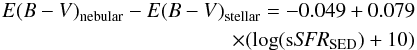 (A.2)Reddy et al. (2015) emphasize that Eq. (A.2) is affected by a large scatter (σ ~ 0.12).
Appendix B: UV β slope and SED fitting procedure
We want to derive the UV β slope as accurately as possible because this quantity is known to be related to the dust attenuation and is also dependent on the age of the stellar population and the star formation history (Leitherer & Heckman 1995; Meurer et al. 1999). To derive the UV β slope, we perform a multiband fitting using the bands between 1500 Å and 2500 Å (Castellano et al. 2012). However, the flux in the z850 band is lower than what we expect from the observed fluxes in the band just blueward and redward z850 (I814 and Y098). We compare theoretical expectation from the MOSDEF attenuation curve and the MW curve (Seaton 1979) with Ion2 observed colors in Fig. B.1. The MW curve exhibits the 2175 Å bump that could explain the flux decrease in the z850 band, while uncertainties are too large to discriminate between a curve with or without the 2175 Å bump. However, Scoville et al. (2015) report that their data are consistent with the presence of the 2175 Å bump, while for Reddy et al. (2015) this presence is only marginal.
We derive the β slope from the UV spectrum, using the wavelength windows described in Calzetti et al. (1994), but excluding the 10th window because it is outside the UV spectrum wavelength coverage. The median flux within each window is calculated and used to fit a linear relation in the observed spectrum, assuming the flux density per unit wavelength Fλ ~ λβ, in units of erg s-1 cm-2 Å-1 (Hathi et al. 2015). The resulting slope is  . It is worth noting that the UV slope from the spectrum is not influenced by the possible 2175 Å bump. The UV slope derived from the spectrum is consistent within 1σ with the β slope derived from multiband fitting of the photometry (−2.20 ± 0.20).
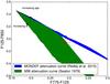 |
Fig. B.1 Range of F775−F125 and F125−F850 colors predicted by BC03 templates and the MOSDEF (Reddy et al. 2015) and MW attenuation curves (Seaton 1979). Ion2 colors are shown by the red square. |
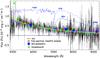 |
Fig. B.2 1D UV spectrum from V15 (black). ACS photometry (blue squares) is shown along with the corresponding transmission curves (V606, i775, I814, and z850, blue dashed lines). We also show the medium-band photometry from the MUSYC survey (green stars, Cardamone et al. 2010). The red dots and associated error bars show the flux derived through the wavelength windows used in Calzetti et al. (1994) to derive the UV β slope. The cyan line denotes the best fit over the Calzetti windows and the violet and yellow lines encompass the 68% uncertainty (β = −2.75, −3.40 and −2.20, respectively). |
Regarding the SED fitting procedure, we use the BC03 templates (Bruzual & Charlot 2003) and we anchor the result to the UV β slope by not taking into account solutions inconsistent with the β slope derived from the UV spectrum within 1σ. We also fix the metallicity to Z = 0.2 Z⊙, which is consistent with the metallicity derived in Sect. 3.2. We test different star formation histories (declining, rising, constant) and attenuation curves (Calzetti, MOSDEF, MW), assuming a Salpeter IMF (Salpeter 1955). The results show that the physical parameters such as stellar mass and age are not strongly affected by the assumptions. Therefore, in this work, we assume a constant star formation history and the MOSDEF attenuation curve. While the β slope is consistent with no or low dust attenuation, we use the relations derived in Reddy et al. (2015) to translate the β slope in color excess. This leads to E(B − V)stellar ≤ 0.04, while the Meurer relation (Meurer et al. 1999) leads to no dust attenuation because of the higher intrinsic β slope in this latter relation.
Created with the Rainbow Navigator tool, https://rainbow.fis.ucm.es/Rainbow_navigator_public/
Acknowledgments
We thank the referee for suggestions that clarify the text and the analysis. We thank M. Tosi, F. Annibali, M. Brusa and H. Atek for useful discussions. We acknowledge the financial contribution from PRIN-INAF 2012. This work has made use of the Rainbow Cosmological Surveys Database, which is operated by the Universidad Complutense de Madrid (UCM), partnered with the University of California Observatories at Santa Cruz (UCO/Lick, UCSC).
References
- Amorín, R. O., Pérez-Montero, E., & Vílchez, J. M. 2010, ApJ, 715, L128 [NASA ADS] [CrossRef] [Google Scholar]
- Amorín, R., Pérez-Montero, E., Vílchez, J. M., & Papaderos, P. 2012, ApJ, 749, 185 [NASA ADS] [CrossRef] [Google Scholar]
- Amorín, R., Grazian, A., Castellano, M., et al. 2014a, ApJ, 788, L4 [NASA ADS] [CrossRef] [Google Scholar]
- Amorín, R., Sommariva, V., Castellano, M., et al. 2014b, A&A, 568, L8 [NASA ADS] [CrossRef] [EDP Sciences] [Google Scholar]
- Amorín, R., Pérez-Montero, E., Contini, T., et al. 2015, A&A, 578, A105 [NASA ADS] [CrossRef] [EDP Sciences] [Google Scholar]
- Annibali, F., Tosi, M., Pasquali, A., et al. 2015, AJ, 150, 143 [NASA ADS] [CrossRef] [Google Scholar]
- Ashby, M. L. N., Willner, S. P., Fazio, G. G., et al. 2013, ApJ, 769, 80 [NASA ADS] [CrossRef] [Google Scholar]
- Ashby, M. L. N., Willner, S. P., Fazio, G. G., et al. 2015, ApJS, 218, 33 [NASA ADS] [CrossRef] [Google Scholar]
- Asplund, M., Grevesse, N., Sauval, A. J., & Scott, P. 2009, ARA&A, 47, 481 [NASA ADS] [CrossRef] [Google Scholar]
- Atek, H., Siana, B., Scarlata, C., et al. 2011, ApJ, 743, 121 [NASA ADS] [CrossRef] [Google Scholar]
- Atek, H., Kunth, D., Schaerer, D., et al. 2014, A&A, 561, A89 [NASA ADS] [CrossRef] [EDP Sciences] [Google Scholar]
- Baldwin, J. A., Phillips, M. M., & Terlevich, R. 1981, PASP, 93, 5 [NASA ADS] [CrossRef] [EDP Sciences] [Google Scholar]
- Balestra, I., Mainieri, V., Popesso, P., et al. 2010, A&A, 512, A12 [NASA ADS] [CrossRef] [EDP Sciences] [Google Scholar]
- Beckwith, S. V. W., Stiavelli, M., Koekemoer, A. M., et al. 2006, AJ, 132, 1729 [NASA ADS] [CrossRef] [Google Scholar]
- Behrens, C., Dijkstra, M., & Niemeyer, J. C. 2014, A&A, 563, A77 [NASA ADS] [CrossRef] [EDP Sciences] [Google Scholar]
- Binette, L., Groves, B., Villar-Martín, M., Fosbury, R. A. E., & Axon, D. J. 2003, A&A, 405, 9 [Google Scholar]
- Borthakur, S., Heckman, T. M., Leitherer, C., & Overzier, R. A. 2014, Science, 346, 216 [NASA ADS] [CrossRef] [Google Scholar]
- Boutsia, K., Grazian, A., Giallongo, E., et al. 2011, ApJ, 736, 41 [NASA ADS] [CrossRef] [Google Scholar]
- Bouwens, R. J., Illingworth, G. D., Oesch, P. A., et al. 2015, ApJ, 811, 140 [NASA ADS] [CrossRef] [Google Scholar]
- Brammer, G. B., Sánchez-Janssen, R., Labbé, I., et al. 2012, ApJ, 758, L17 [NASA ADS] [CrossRef] [Google Scholar]
- Bridge, C. R., Teplitz, H. I., Siana, B., et al. 2010, ApJ, 720, 465 [NASA ADS] [CrossRef] [Google Scholar]
- Brinchmann, J., Charlot, S., White, S. D. M., et al. 2004, MNRAS, 351, 1151 [NASA ADS] [CrossRef] [Google Scholar]
- Bruzual, G., & Charlot, S. 2003, MNRAS, 344, 1000 [NASA ADS] [CrossRef] [Google Scholar]
- Caccianiga, A., & Severgnini, P. 2011, MNRAS, 415, 1928 [NASA ADS] [CrossRef] [Google Scholar]
- Calzetti, D., Kinney, A. L., & Storchi-Bergmann, T. 1994, ApJ, 429, 582 [NASA ADS] [CrossRef] [Google Scholar]
- Calzetti, D., Armus, L., Bohlin, R. C., et al. 2000, ApJ, 533, 682 [NASA ADS] [CrossRef] [Google Scholar]
- Cardamone, C., Schawinski, K., Sarzi, M., et al. 2009, MNRAS, 399, 1191 [NASA ADS] [CrossRef] [Google Scholar]
- Cardamone, C. N., van Dokkum, P. G., Urry, C. M., et al. 2010, ApJS, 189, 270 [NASA ADS] [CrossRef] [Google Scholar]
- Cardelli, J. A., Clayton, G. C., & Mathis, J. S. 1989, ApJ, 345, 245 [NASA ADS] [CrossRef] [Google Scholar]
- Cassata, P., Le Fèvre, O., Charlot, S., et al. 2013, A&A, 556, A68 [NASA ADS] [CrossRef] [EDP Sciences] [Google Scholar]
- Castellano, M., Fontana, A., Grazian, A., et al. 2012, A&A, 540, A39 [NASA ADS] [CrossRef] [EDP Sciences] [Google Scholar]
- Cen, R., & Kimm, T. 2015, ApJ, 801, L25 [NASA ADS] [CrossRef] [Google Scholar]
- Christensen, L., Laursen, P., Richard, J., et al. 2012, MNRAS, 427, 1973 [NASA ADS] [CrossRef] [Google Scholar]
- de Barros, S., Reddy, N., & Shivaei, I. 2015, ApJ, submitted [arXiv:1509.05055] [Google Scholar]
- De Breuck, C., Röttgering, H., Miley, G., van Breugel, W., & Best, P. 2000, A&A, 362, 519 [NASA ADS] [Google Scholar]
- Domínguez, A., Siana, B., Henry, A. L., et al. 2013, ApJ, 763, 145 [NASA ADS] [CrossRef] [Google Scholar]
- Erb, D. K., Steidel, C. C., Shapley, A. E., et al. 2006, ApJ, 647, 128 [NASA ADS] [CrossRef] [Google Scholar]
- Ferland, G. J., Porter, R. L., van Hoof, P. A. M., et al. 2013, Rev. Mex. Astron. Astrophys., 49, 137 [Google Scholar]
- Finkelstein, S. L., Papovich, C., Dickinson, M., et al. 2013, Nature, 502, 524 [NASA ADS] [CrossRef] [Google Scholar]
- Fontana, A., Dunlop, J. S., Paris, D., et al. 2014, A&A, 570, A11 [NASA ADS] [CrossRef] [EDP Sciences] [Google Scholar]
- Fontanot, F., Cristiani, S., Pfrommer, C., Cupani, G., & Vanzella, E. 2014, MNRAS, 438, 2097 [NASA ADS] [CrossRef] [Google Scholar]
- Förster Schreiber, N. M., Genzel, R., Bouché, N., et al. 2009, ApJ, 706, 1364 [NASA ADS] [CrossRef] [Google Scholar]
- Garnett, D. R., Shields, G. A., Peimbert, M., et al. 1999, ApJ, 513, 168 [NASA ADS] [CrossRef] [Google Scholar]
- Giallongo, E., Grazian, A., Fiore, F., et al. 2015, A&A, 578, A83 [NASA ADS] [CrossRef] [EDP Sciences] [Google Scholar]
- Giavalisco, M., Ferguson, H. C., Koekemoer, A. M., et al. 2004, ApJ, 600, L93 [NASA ADS] [CrossRef] [Google Scholar]
- Gräfener, G., & Vink, J. S. 2015, A&A, 578, L2 [NASA ADS] [CrossRef] [EDP Sciences] [Google Scholar]
- Grazian, A., Fontana, A., Santini, P., et al. 2015, A&A, 575, A96 [NASA ADS] [CrossRef] [EDP Sciences] [Google Scholar]
- Grogin, N. A., Kocevski, D. D., Faber, S. M., et al. 2011, ApJS, 197, 35 [NASA ADS] [CrossRef] [Google Scholar]
- Guo, Y., Ferguson, H. C., Giavalisco, M., et al. 2013, ApJS, 207, 24 [NASA ADS] [CrossRef] [Google Scholar]
- Hainline, K. N., Shapley, A. E., Greene, J. E., & Steidel, C. C. 2011, ApJ, 733, 31 [NASA ADS] [CrossRef] [Google Scholar]
- Hathi, N. P., Le Fèvre, O., Ilbert, O., et al. 2015, A&A, submitted [arXiv:1503.01753] [Google Scholar]
- Hayes, M., Östlin, G., Duval, F., et al. 2014, ApJ, 782, 6 [NASA ADS] [CrossRef] [Google Scholar]
- Heckman, T. M., Borthakur, S., Overzier, R., et al. 2011, ApJ, 730, 5 [Google Scholar]
- Henry, A., Scarlata, C., Martin, C. L., & Erb, D. 2015, ApJ, 809, 19 [NASA ADS] [CrossRef] [Google Scholar]
- Holden, B. P., Oesch, P. A., Gonzalez, V. G., et al. 2014, ApJ, submitted [arXiv:1401.5490] [Google Scholar]
- Inoue, A. K., & Iwata, I. 2008, MNRAS, 387, 1681 [NASA ADS] [CrossRef] [Google Scholar]
- Inoue, A. K., Shimizu, I., Iwata, I., & Tanaka, M. 2014, MNRAS, 442, 1805 [NASA ADS] [CrossRef] [Google Scholar]
- Iwata, I., Inoue, A. K., Matsuda, Y., et al. 2009, ApJ, 692, 1287 [NASA ADS] [CrossRef] [Google Scholar]
- James, B. L., Pettini, M., Christensen, L., et al. 2014, MNRAS, 440, 1794 [NASA ADS] [CrossRef] [Google Scholar]
- Jaskot, A. E., & Oey, M. S. 2013, ApJ, 766, 91 [NASA ADS] [CrossRef] [Google Scholar]
- Jaskot, A. E., & Oey, M. S. 2014, ApJ, 791, L19 [NASA ADS] [CrossRef] [Google Scholar]
- Jones, T., Stark, D. P., & Ellis, R. S. 2012, ApJ, 751, 51 [NASA ADS] [CrossRef] [Google Scholar]
- Jones, T. A., Ellis, R. S., Schenker, M. A., & Stark, D. P. 2013, ApJ, 779, 52 [NASA ADS] [CrossRef] [Google Scholar]
- Juneau, S., Dickinson, M., Alexander, D. M., & Salim, S. 2011, ApJ, 736, 104 [NASA ADS] [CrossRef] [Google Scholar]
- Juneau, S., Bournaud, F., Charlot, S., et al. 2014, ApJ, 788, 88 [NASA ADS] [CrossRef] [Google Scholar]
- Kashino, D., Silverman, J. D., Rodighiero, G., et al. 2013, ApJ, 777, L8 [NASA ADS] [CrossRef] [Google Scholar]
- Kennicutt, Jr., R. C. 1998, ARA&A, 36, 189 [Google Scholar]
- Koekemoer, A. M., Faber, S. M., Ferguson, H. C., et al. 2011, ApJS, 197, 36 [NASA ADS] [CrossRef] [Google Scholar]
- Kulas, K. R., Shapley, A. E., Kollmeier, J. A., et al. 2012, ApJ, 745, 33 [NASA ADS] [CrossRef] [Google Scholar]
- Labbé, I., Oesch, P. A., Bouwens, R. J., et al. 2013, ApJ, 777, L19 [NASA ADS] [CrossRef] [Google Scholar]
- Lamareille, F., Mouhcine, M., Contini, T., Lewis, I., & Maddox, S. 2004, MNRAS, 350, 396 [NASA ADS] [CrossRef] [Google Scholar]
- Lanzuisi, G., Perna, M., Delvecchio, I., et al. 2015, A&A, 578, A120 [NASA ADS] [CrossRef] [EDP Sciences] [Google Scholar]
- Leitherer, C., & Heckman, T. M. 1995, ApJS, 96, 9 [NASA ADS] [CrossRef] [Google Scholar]
- Lutz, D., Maiolino, R., Spoon, H. W. W., & Moorwood, A. F. M. 2004, A&A, 418, 465 [NASA ADS] [CrossRef] [EDP Sciences] [Google Scholar]
- Ly, C., Malkan, M. A., Nagao, T., et al. 2014, ApJ, 780, 122 [NASA ADS] [CrossRef] [Google Scholar]
- Malkan, M., Webb, W., & Konopacky, Q. 2003, ApJ, 598, 878 [NASA ADS] [CrossRef] [Google Scholar]
- Maseda, M. V., van der Wel, A., Rix, H.-W., et al. 2014, ApJ, 791, 17 [CrossRef] [Google Scholar]
- Meurer, G. R., Heckman, T. M., & Calzetti, D. 1999, ApJ, 521, 64 [NASA ADS] [CrossRef] [Google Scholar]
- Mostardi, R. E., Shapley, A. E., Nestor, D. B., et al. 2013, ApJ, 779, 65 [NASA ADS] [CrossRef] [Google Scholar]
- Mostardi, R. E., Shapley, A. E., Steidel, C. C., et al. 2015, ApJ, 810, 107 [NASA ADS] [CrossRef] [Google Scholar]
- Nagao, T., Maiolino, R., & Marconi, A. 2006, A&A, 459, 85 [NASA ADS] [CrossRef] [EDP Sciences] [Google Scholar]
- Nakajima, K., & Ouchi, M. 2014, MNRAS, 442, 900 [NASA ADS] [CrossRef] [Google Scholar]
- Nestor, D. B., Shapley, A. E., Steidel, C. C., & Siana, B. 2011, ApJ, 736, 18 [NASA ADS] [CrossRef] [Google Scholar]
- Nestor, D. B., Shapley, A. E., Kornei, K. A., Steidel, C. C., & Siana, B. 2013, ApJ, 765, 47 [NASA ADS] [CrossRef] [Google Scholar]
- Nonino, M., Dickinson, M., Rosati, P., et al. 2009, ApJS, 183, 244 [NASA ADS] [CrossRef] [Google Scholar]
- Oesch, P. A., van Dokkum, P. G., Illingworth, G. D., et al. 2015, ApJ, 804, L30 [Google Scholar]
- Oke, J. B., & Gunn, J. E. 1983, ApJ, 266, 713 [NASA ADS] [CrossRef] [Google Scholar]
- Ono, Y., Ouchi, M., Mobasher, B., et al. 2012, ApJ, 744, 83 [NASA ADS] [CrossRef] [Google Scholar]
- Osterbrock, D. E. 1989, Astrophysics of gaseous nebulae and active galactic nuclei (Mill Valley, CA: University Science Books) [Google Scholar]
- Pallottini, A., Ferrara, A., Pacucci, F., et al. 2015, MNRAS, 453, 2465 [NASA ADS] [Google Scholar]
- Panessa, F., Bassani, L., Cappi, M., et al. 2006, A&A, 455, 173 [NASA ADS] [CrossRef] [EDP Sciences] [Google Scholar]
- Pérez-Montero, E. 2014, MNRAS, 441, 2663 [NASA ADS] [CrossRef] [Google Scholar]
- Pope, A., Chary, R.-R., Alexander, D. M., et al. 2008, ApJ, 675, 1171 [Google Scholar]
- Popesso, P., Dickinson, M., Nonino, M., et al. 2009, A&A, 494, 443 [NASA ADS] [CrossRef] [EDP Sciences] [Google Scholar]
- Price, S. H., Kriek, M., Brammer, G. B., et al. 2014, ApJ, 788, 86 [NASA ADS] [CrossRef] [Google Scholar]
- Rauch, M., Becker, G. D., Haehnelt, M. G., et al. 2011, MNRAS, 418, 1115 [NASA ADS] [CrossRef] [Google Scholar]
- Reddy, N. A., Erb, D. K., Pettini, M., Steidel, C. C., & Shapley, A. E. 2010, ApJ, 712, 1070 [NASA ADS] [CrossRef] [Google Scholar]
- Reddy, N. A., Kriek, M., Shapley, A. E., et al. 2015, ApJ, 806, 259 [NASA ADS] [CrossRef] [Google Scholar]
- Roberts-Borsani, G. W., Bouwens, R. J., Oesch, P. A., et al. 2015, ApJ, submitted [arXiv:1506.00854] [Google Scholar]
- Robertson, B. E., Ellis, R. S., Furlanetto, S. R., & Dunlop, J. S. 2015, ApJ, 802, L19 [NASA ADS] [CrossRef] [Google Scholar]
- Rousselot, P., Lidman, C., Cuby, J.-G., Moreels, G., & Monnet, G. 2000, A&A, 354, 1134 [NASA ADS] [Google Scholar]
- Rujopakarn, W., Rieke, G. H., Papovich, C. J., et al. 2012, ApJ, 755, 168 [NASA ADS] [CrossRef] [Google Scholar]
- Salpeter, E. E. 1955, ApJ, 121, 161 [Google Scholar]
- Santini, P., Fontana, A., Grazian, A., et al. 2009, A&A, 504, 751 [NASA ADS] [CrossRef] [EDP Sciences] [Google Scholar]
- Schaerer, D., & de Barros, S. 2010, A&A, 515, A73 [NASA ADS] [CrossRef] [EDP Sciences] [Google Scholar]
- Scoville, N., Faisst, A., Capak, P., et al. 2015, ApJ, 800, 108 [NASA ADS] [CrossRef] [Google Scholar]
- Seaton, M. J. 1979, MNRAS, 187, 73P [NASA ADS] [CrossRef] [Google Scholar]
- Shapley, A. E., Steidel, C. C., Pettini, M., & Adelberger, K. L. 2003, ApJ, 588, 65 [NASA ADS] [CrossRef] [Google Scholar]
- Shapley, A. E., Steidel, C. C., Pettini, M., Adelberger, K. L., & Erb, D. K. 2006, ApJ, 651, 688 [NASA ADS] [CrossRef] [Google Scholar]
- Shivaei, I., Reddy, N. A., Steidel, C. C., & Shapley, A. E. 2015, ApJ, 804, 149 [NASA ADS] [CrossRef] [Google Scholar]
- Siana, B., Teplitz, H. I., Ferguson, H. C., et al. 2010, ApJ, 723, 241 [NASA ADS] [CrossRef] [Google Scholar]
- Siana, B., Shapley, A. E., Kulas, K. R., et al. 2015, ApJ, 804, 17 [NASA ADS] [CrossRef] [Google Scholar]
- Smit, R., Bouwens, R. J., Labbé, I., et al. 2014, ApJ, 784, 58 [NASA ADS] [CrossRef] [Google Scholar]
- Smit, R., Bouwens, R. J., Franx, M., et al. 2015, ApJ, 801, 122 [NASA ADS] [CrossRef] [Google Scholar]
- Sobral, D., Matthee, J., Darvish, B., et al. 2015, ApJ, 808, 139 [NASA ADS] [CrossRef] [Google Scholar]
- Stark, D. P., Richard, J., Siana, B., et al. 2014, MNRAS, 445, 3200 [NASA ADS] [CrossRef] [Google Scholar]
- Stasińska, G., Izotov, Y., Morisset, C., & Guseva, N. 2015, A&A, 576, A83 [NASA ADS] [CrossRef] [EDP Sciences] [Google Scholar]
- Steidel, C. C., Pettini, M., & Adelberger, K. L. 2001, ApJ, 546, 665 [NASA ADS] [CrossRef] [Google Scholar]
- Steidel, C. C., Rudie, G. C., Strom, A. L., et al. 2014, ApJ, 795, 165 [NASA ADS] [CrossRef] [Google Scholar]
- Storey, P. J., & Zeippen, C. J. 2000, MNRAS, 312, 813 [Google Scholar]
- Szécsi, D., Langer, N., Yoon, S.-C., et al. 2015, A&A, 581, A15 [NASA ADS] [CrossRef] [EDP Sciences] [Google Scholar]
- van der Wel, A., Straughn, A. N., Rix, H.-W., et al. 2011, ApJ, 742, 111 [NASA ADS] [CrossRef] [Google Scholar]
- Vanzella, E., Giavalisco, M., Inoue, A. K., et al. 2010a, ApJ, 725, 1011 [NASA ADS] [CrossRef] [Google Scholar]
- Vanzella, E., Siana, B., Cristiani, S., & Nonino, M. 2010b, MNRAS, 404, 1672 [NASA ADS] [Google Scholar]
- Vanzella, E., Pentericci, L., Fontana, A., et al. 2011, ApJ, 730, L35 [NASA ADS] [CrossRef] [Google Scholar]
- Vanzella, E., Guo, Y., Giavalisco, M., et al. 2012, ApJ, 751, 70 [NASA ADS] [CrossRef] [Google Scholar]
- Vanzella, E., Fontana, A., Pentericci, L., et al. 2014a, A&A, 569, A78 [NASA ADS] [CrossRef] [EDP Sciences] [PubMed] [Google Scholar]
- Vanzella, E., Fontana, A., Zitrin, A., et al. 2014b, ApJ, 783, L12 [NASA ADS] [CrossRef] [Google Scholar]
- Vanzella, E., de Barros, S., Castellano, M., et al. 2015, A&A, 576, A116 [NASA ADS] [CrossRef] [EDP Sciences] [Google Scholar]
- Verhamme, A., Orlitová, I., Schaerer, D., & Hayes, M. 2015, A&A, 578, A7 [NASA ADS] [CrossRef] [EDP Sciences] [Google Scholar]
- Vignali, C., Alexander, D. M., Gilli, R., & Pozzi, F. 2010, MNRAS, 404, 48 [NASA ADS] [Google Scholar]
- Windhorst, R. A., Cohen, S. H., Hathi, N. P., et al. 2011, ApJS, 193, 27 [NASA ADS] [CrossRef] [Google Scholar]
- Worseck, G., Prochaska, J. X., O’Meara, J. M., et al. 2014, MNRAS, 445, 1745 [NASA ADS] [CrossRef] [Google Scholar]
- Yang, H., Malhotra, S., Gronke, M., et al. 2015, ApJ, submitted [arXiv:1506.02885] [Google Scholar]
- Zackrisson, E., Inoue, A. K., & Jensen, H. 2013, ApJ, 777, 39 [NASA ADS] [CrossRef] [Google Scholar]
- Zitrin, A., Labbé, I., Belli, S., et al. 2015, ApJ, 810, L12 [NASA ADS] [CrossRef] [Google Scholar]
All Tables
All Figures
|
Fig. 1 Postage stamps of Ion2 in B435, V606, i775, z850, H160, IRAC 3.5 μm, IRAC 4.5 μm, IRAC 5.8 μm, IRAC 8.0 μm, and MIPS 24 μm. The sizes of the images are 4′′ × 4′′ for the HST bands and 20′′ × 20′′ for the Spitzer bands. |
| In the text | |
|
Fig. 2 Two-dimensional LR VIMOS UV spectrum of Ion2 with different cuts to emphasize the spectral features Lyα and Lyβ (bottom) and the Lyman continuum λ< 912 Å, in the range 855–910 Å (top, vertical dotted blue lines). On the left, we show the moving average calculated within a rectangular aperture (855−910 Å × 1.25′′, red-dotted rectangle) in the spatial direction divided by its rms on the left side. A signal is detected at λ< 912 Å with S/N> 5. The inset shows the pixel distribution of the background after sky-subtraction in the region 855–910 Å (derived from the S/N spectrum). The distribution is symmetric (skewness = −0.016) with the mean and median close to zero, +0.0057 and −0.014, respectively. No significant systematic effects are present. |
| In the text | |
|
Fig. 3 Ground-based VLT/VIMOS U-band observation of Ion2 at a resolution of 0.2′′/pixel (left panel). The contour of the system (derived from the ACS/i775 band, center panel) is indicated and superimposed in blue onto the VIMOS U-image and onto the HAWK-I Ks image (right panel). The cutouts are 2.6′′ × 2.6′′. |
| In the text | |
|
Fig. 4 Two- and one-dimensional near-infrared spectra of Ion2 in the MOSFIRE H- and K-band. Two insets show the regions where Hβ and the [O ii]λ3727 doublet are expected from the redshift. The gray stripes in the one-dimensional spectra indicate the position of the sky lines. |
| In the text | |
|
Fig. 5 Observed and simulated two-dimensional MOSFIRE spectrum, with the observed [O iii]λ5007 line replicated at different wavelength positions with different dimming factors (DIM). See text. |
| In the text | |
|
Fig. 6 1D and 2D UV VLT/VIMOS MR spectra. The transparent blue stripes indicate the positions of the emission sky lines. The transparent red stripes indicate the telluric molecular sky absorptions bands, B- and A-bands at ~6900 Å and ~7600 Å. In the same panel, three 2D spectra are shown, the reduced, rms and signal-to-noise ratio, from bottom to top. The inset on the left side shows the double-peaked Lya line (from V15). In the bottom right a zoom-in around the He iiλ1640 and O iii]λ1666 positions is shown. Their detections remain tentative. In the bottom left, the 1D spectrum shows the relative Lyα flux in comparison with other lines. |
| In the text | |
|
Fig. 7 Comparison of the metallicity and ionization parameter (U = q/c) between the mean sample properties from Nakajima & Ouchi (2014) and Ion2 with 1σ uncertainties. Ion2 is compared to local galaxies from the SDSS survey, a galaxy sample at z ~ 1, a Lyman break galaxy (LBG) sample at z ~ 2.5, a Lyman alpha emitter (LAE) sample at z ~ 2.5, local Lyman break analogues (LBAs), LyC emitters, and Green Peas (GPs). See Nakajima & Ouchi (2014) and references therein for a complete description of these samples. |
| In the text | |
|
Fig. 8 Observed Ion2 SED (black and red dots). We show the best SED fit in blue and the integrated fluxes with blue crosses. We exclude photometric points (in red) affected by the IGM and strong emission lines (Lyα, [O iii]) from the SED fitting. The arrow indicates the 1σ upper limit. |
| In the text | |
|
Fig. 9 Velocity profiles of [O iii]λ5007 and Lyα lines relative to systemic. The [O iii]λ5007 line is shown in black, the Lyα first order in red, and the Lyα second order with the dashed blue line. The positions and widths of the sky lines are indicated by gray stripes. |
| In the text | |
|
Fig. B.1 Range of F775−F125 and F125−F850 colors predicted by BC03 templates and the MOSDEF (Reddy et al. 2015) and MW attenuation curves (Seaton 1979). Ion2 colors are shown by the red square. |
| In the text | |
|
Fig. B.2 1D UV spectrum from V15 (black). ACS photometry (blue squares) is shown along with the corresponding transmission curves (V606, i775, I814, and z850, blue dashed lines). We also show the medium-band photometry from the MUSYC survey (green stars, Cardamone et al. 2010). The red dots and associated error bars show the flux derived through the wavelength windows used in Calzetti et al. (1994) to derive the UV β slope. The cyan line denotes the best fit over the Calzetti windows and the violet and yellow lines encompass the 68% uncertainty (β = −2.75, −3.40 and −2.20, respectively). |
| In the text | |
Current usage metrics show cumulative count of Article Views (full-text article views including HTML views, PDF and ePub downloads, according to the available data) and Abstracts Views on Vision4Press platform.
Data correspond to usage on the plateform after 2015. The current usage metrics is available 48-96 hours after online publication and is updated daily on week days.
Initial download of the metrics may take a while.