| Issue |
A&A
Volume 584, December 2015
|
|
|---|---|---|
| Article Number | A110 | |
| Number of page(s) | 16 | |
| Section | Planets and planetary systems | |
| DOI | https://doi.org/10.1051/0004-6361/201526921 | |
| Published online | 01 December 2015 | |
How do giant planetary cores shape the dust disk?
HL Tauri system
Institut für Astronomie und Astrophysik, Kepler Center, Universität Tübingen, Auf der Morgenstelle 10, 72076 Tübingen, Germany
e-mail: This email address is being protected from spambots. You need JavaScript enabled to view it.
Received: 9 July 2015
Accepted: 2 October 2015
Abstract
Context. We have been observing, thanks to ALMA, the dust distribution in the region of active planet formation around young stars. This is a powerful tool that can be used to connect observations with theoretical models and improve our understanding of the processes at play.
Aims. We want to test how a multiplanetary system shapes its birth disk and to study the influence of the planetary masses and particle sizes on the final dust distribution. Moreover, we apply our model to the HL Tau system in order to obtain some insights on the physical parameters of the planets that are able to create the observed features.
Methods. We follow the evolution of a population of dust particles, treated as Lagrangian particles, in two-dimensional locally isothermal disks where two equal-mass planets are present. The planets are kept in fixed orbits and they do not accrete mass.
Results. The outer planet plays a major role in removing the dust particles in the co-orbital region of the inner planet and in forming a particle ring which have a steeper density gradient close to the gap edge respect to the single-planet scenario, promoting the development of vortices. The ring and gap width depend strongly on the planetary mass and particle stopping times, and for the more massive cases on the ring clumps in few stable points that are able to collect a high mass fraction. The features observed in the HL Tau system can be explained through the presence of several massive cores that shape the dust disk where the inner planet(s) have a mass of the order of 0.07 MJup and the outer one(s) of the order of 0.35 MJup. These values can be significantly lower if the disk mass turns out to be less than previously estimated. By decreasing the disk mass by a factor of 10, we obtain similar gap widths for planets with a mass of 10 M⊕ and 20 M⊕ for the inner and outer planets, respectively. Although the particle gaps are prominent, the expected gaseous gaps are barely visible.
Key words: accretion, accretion disks / hydrodynamics / planet-disk interactions / protoplanetary disks / stars: pre-main sequence
© ESO, 2015
1. Introduction
The planetary cores of giant planets form on a timescale of ~1 Myr. In this relatively short time span, a huge number of processes take place, allowing a swarm of small dust particles to grow several order of magnitudes in size and mass before the gas disk disappears. Until now, the only observational constraints that we had to test planet formation models were the gas and dust emissions from protoplanetary nebulae on large scales (of the order of ~100 au) and the final stage of planet formation through the detection of full-fledged planetary systems. Thanks to the recent advent of a new generation of radio telescopes, like the Atacama Large Millimeter Array (ALMA), we are starting to obtain pristine images of the formation process itself that resolve the dust component of protoplanetary disks in the region of active planet formation around young stars.
An outstanding example of this giant leap in the observational data is the young HL Tau system, imaged by ALMA in Bands 3, 6, and 7 (respectively at wavelengths 2.9, 1.3, and 0.87 mm) with a spatial resolution of up to 3.5 au. Several features can be seen in the young protoplanetary disk, but the most striking is the presence of several axysimmetric rings in the mm dust disk (ALMA Partnership et al. 2015). Although different mechanisms can be responsible of the observed features (Flock et al. 2015; Zhang et al. 2015), the most straightforward explanation for the ring formation, in the sense that others mechanism require specific initial conditions that reduce their general applicability, is the presence of several planetary cores that grow in their birth disk and shape its dust content. In order to have a particle concentration at a particular region, we need a steep pressure gradient in the gaseous disk which can trap “sufficiently” decoupled particles by changing their migration direction. A long-lived high-pressure region can be created even by small mass planets (Paardekooper & Mellema 2004), which can effectively carve a deep dust gap and concentrate particles at the gap edges and at corotation in tadpole orbits (Paardekooper 2007; Fouchet et al. 2007).
The aim of this paper is to test how two giant planetary cores shape the dust disk in which they are born, implementing a particle population in the 2D hydro code fargo (Masset 2000), and study the influence of the planetary masses and particle sizes on the final disk distribution. Moreover, we apply our model to the HL Tau system in order to obtain some insights on the physical parameters of the planets creating the observed features.
This paper is organised as follows. In Sect. 2 we discuss under which physical conditions a planet is capable of opening a gap in the dust and gaseous disk in order to define the important physical scales for our model. In Sect. 3 we define the model adopted for the gas drag. The setup of our simulations is explained in Sect. 4, and the main results are outlined in Sect. 5. Finally, in Sect. 6 we discuss our results and their implications and limitation, while the major outcomes are highlighted in Sect. 7.
2. Background
In order to set up our model, we need first to determine the minimum mass of a planetary core that is able to open up a gap in the gaseous and dust disk for a given set of disk parameters, and the timescale of this opening. In particular, we want to understand the influence of the different physical processes modelled on the outcome of the simulation.
2.1. Theory of gap formation
The theory of gap formation in gaseous disks has been studied extensively in the past, and there are a set of general criteria that a planet must fulfil in order to carve a gap. However, the process of opening a gap in the dust disk is more complicated to model since it depends strongly on the coupling between the dust and the gaseous media, and this problem has been tackled only recently.
2.1.1. Gaseous gap
The torque exchange between the disk and the planet adds angular momentum to the outer disk regions and removes it from the inner ones. As a result, the disk structure is modified in the regions close to the planet and, given a minimum core mass and enough time, a gap develops.
The timescale needed to open a gap of half width xs can be roughly estimated from the impulse approximation (Lin & Papaloizou 1979). The total torque acting on a planet of mass Mp and semi-major axis a due to its interaction with the outer disk of surface density Σ is (Lin & Papaloizou 1979; Papaloizou & Terquem 2006) 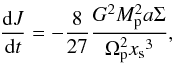 (1)where
  is the planet orbital frequency around a star of mass M⋆. The angular momentum that must be added to the disk in order to remove the gas inside the gap is
 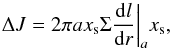 (2)where
  is the gas specific angular momentum. Thus, the gap opening time can be estimated as
 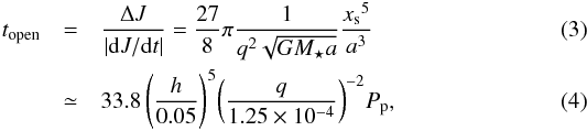 where q = Mp/M⋆ is the planet-to-star mass ratio, and we assumed that the minimum half width of the gap should be xs = H, where H is the effective disk thickness and h = H/r is the normalised disk scale height. All values are evaluated at the planet location and the final estimate of the opening time is given in units of the planet orbital time Pp. Although this is a rough estimate, it has been shown with more detailed descriptions that the order of magnitude obtained is correct.
Based on this criterion and given enough time, even a small core can open a gap in an inviscid disk, but we need to quantify the magnitude of the competing factors that act to prevent or promote its development to obtain a better estimate of the gap opening timescale and the minimum mass ratio.
Thermal condition.
The assumption made for the minimum gap half width in Eq. (3) is necessary to allow non-linear dissipation of waves generated by the planet (Korycansky & Papaloizou 1996) and to avoid dynamical instabilities at the planet location (Papaloizou & Lin 1984); these conditions are necessary to clear the regions close to the planet location. This condition, called thermal condition, translates into a first criterion for opening up a gap for a 2D disk (Masset et al. 2006), 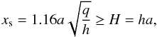 (5)which corresponds to a minimum planet to star mass ratio of
 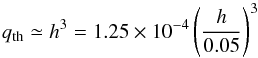 (6)and a related thermal mass
  (7)
(7)
Viscous condition.
The viscous diffusion acts to smooth out sharp radial gradients in the disk surface density and prevents the gap clearing mechanism. The time needed by viscous forces to close up a gap of width xs is given by the diffusion timescale for a viscous fluid, which can be derived directly from the Navier-Stokes equation in cylindrical polar coordinates (see e.g. Armitage 2010) 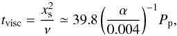 (8)where ν is the kinematic viscosity and
  is the Shakura-Sunyaev parameter that measures the efficiency of angular momentum transport due to turbulence.
The minimum mass qvisc needed to open a gap in a viscous disk is obtained by comparing the opening time due to the torque interaction, Eq. (3) with the viscous closing time Eq. (8) (Lin & Papaloizou 1986, 1993): 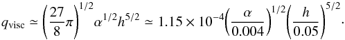 (9)Thus, for the parameters chosen, the viscous condition is very similar to the thermal condition.
Generalised condition.
A more general semi-analytic criterion that takes into account the balance between pressure, gravitational, and viscous torques for a planet on a fixed circular orbit has also been derived (Lin & Papaloizou 1993; Crida et al. 2006), 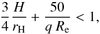 (10)where rH = a(q/ 3)1/3 is the Hill radius and Re is the Reynolds number. Using the previous relation and plugging in the parameters used in our analysis, we found that the minimum mass ratio is q ≃ 10-3. However, this criterion was derived for low planetary masses in low viscosity disks, and the behaviour might be considerably different if these parameters are changed. Moreover, this condition defines a gap as a drop in the mass density to 10% of the unperturbed density at the planet’s location, but even a less dramatic depletion of mass affect planet-disk interaction and so it could be detected.
2.1.2. Dust gap
In order to create a gap in the dust disk we need a radial pressure structure induced by the planet. A very shallow gap in the gas will also change the drift speed of the dust particles significantly (Whipple 1972; Weidenschilling 1977) favouring the formation of a particle gap. Thus, the minimum mass needed to open up a gap in the dust disk is a fraction of the one needed to clear a gap in the gas. Paardekooper & Mellema (2004, 2006) performed extensive 2D simulations, treating the dust as a pressureless fluid (a good approximation for tightly coupled particles), and they found that a planet more massive than 0.05 MJup = 0.38 Mth can open a gap in a mm-sized disk. Furthermore, the dust gap opening time for this lower mass case was 50 Pp, which is about half the timescale needed to open a gas gap. Previous studies also found a clear dependence of the gap width with the core mass, where larger planets open wider gaps (Paardekooper & Mellema 2006; Zhu et al. 2014). Finally, there are some contrasting results regarding the dependence of the gap width on the particle size (Paardekooper & Mellema 2006), but it seems that for less coupled particles the gap is wider for larger particles (Fouchet et al. 2007).
3. Model
As a result of drag forces, solid particles and gaseous molecules exchange momentum. This effect depends strongly on the condition of the gas and on shape, size, and velocity of the particle. For the sake of simplicity we limit ourselves to spherical particles. The drag force always acts in the direction opposite to the relative velocity.
The regime that describes a particular system is defined by any two of three non-dimensional parameters. The Knudsen number K = λ/s is the ratio of two characteristic length scales of the system: the mean free path of the gas molecules λ and the particle size s. The Mach number M = vr/cs is the ratio between the relative velocity between particles and gas vr and the gas sound speed cs. Finally, the Reynolds number Re is related to different physical properties of the particle and gaseous media,  (11)where νm is the gas molecular viscosity, defined as
  (12)here m0 and
  are the mass and mean thermal velocity of the gas molecules and σ is their collisional cross section.
There are two main regimes of the drag forces: the Stokes regime and the Epstein regime.
3.1. Stokes regime
For small Knudsen numbers, the particles experience the gas as a fluid. The drag force of a viscous medium with density ρg(rp) acting on a spherical dust particle with radius s can be modelled as (Landau & Lifshitz 1959)  (13)where the drag coefficient CD is defined for the various regimes described above as (Whipple 1972; Weidenschilling 1977)
  (14)for low Mach numbers; however, high values are not expected for our choice of the parameter space in this regime.
3.2. Epstein regime
For small Knudsen numbers, the interaction between particles and single gas molecule becomes important. It can be modelled as (Epstein 1924)  (15)
(15)
3.3. General law
The transition between the Epstein and Stokes regimes occurs for a particle of size s = 9λ/ 4, which in our case is an m size particle in the inner disk, where the mean free path of the gas molecules is defined as (Haghighipour & Boss 2003) ![Mathematical equation: \begin{equation} \lambda = \frac{m_0}{\pi a_0^2\rho_\mathrm{g}(r)} = \frac{4.72 \times 10^{-9}}{\rho_\mathrm{g}} [{\rm cm}] \end{equation}](/articles/aa/full_html/2015/12/aa26921-15/aa26921-15-eq65.png) (16)for a molecular hydrogen particle with a0 = 1.5 × 108 cm. To model a broad range of particles sizes we adopt a linear combination of Stokes and Epstein regimes (Supulver & Lin 2000; Haghighipour & Boss 2003),
(16)for a molecular hydrogen particle with a0 = 1.5 × 108 cm. To model a broad range of particles sizes we adopt a linear combination of Stokes and Epstein regimes (Supulver & Lin 2000; Haghighipour & Boss 2003),  (17)where the factor f is related to the Knudsen number and is defined as
  (18)
(18)
3.4. Stopping time
An important parameter to evaluate the strength of the drag force is the stopping time ts, which can be defined as  (19)where ms is the mass of the single dust particle of density ρs and, in the Epstein regime, the stopping time can be expressed as
  (20)It is also useful to derive a non-dimensional stopping time (or Stokes number) as
  (21)
(21)
4. Setup
We used the fargo code (Masset 2000; Baruteau & Masset 2008), modified in order to take into account the evolution of partially decoupled particles. An infinitesimally thin disk around a star resembling the observed HL Tau system (Kwon et al. 2011) is modelled. Thus, the vertically integrated versions of the hydrodynamical equations are solved in cylindrical coordinates (r,φ,z) centred on the star where the disk lies in the equatorial plane (z = 0). The resolution adopted in the main simulations is 256 × 512 with 250 000 dust particles for each size, although we also tried doubling the resolution to test whether our results were resolution dependent.
4.1. Gas component
The initial disk is axisymmetric and extends from 0.1 to 4 in code units, where the unit of length is 25 au. The gas moves with azimuthal velocity given by the Keplerian speed around a central star of mass 1 (0.55 M⊙), corrected for the rotating velocity of the coordinate system. We assume no initial radial motion of the gas since a thin Keplerian disk is radially in equilibrium as gravitational and centrifugal forces approximately balance because the pressure effects are small. The initial surface density profile is given by  (22)where Σ0 is the surface density at r = 1 such that the total disk mass is equal to 0.24 (0.13 M⊙) in order to match the value found by Kwon et al. (2011). The disk is modelled with a locally isothermal equation of state, which keeps the initial temperature stratification constant throughout the whole simulation. We assumed a constant aspect ratio H/r = 0.05, which corresponds to a temperature profile
  (23)We introduce a density floor of Σfloor = 10-9 Σ0 to prevent numerical problems. For the inner boundary we applied a zero-gradient outflow condition, while for the outer boundary we adopted a non-reflecting boundary condition. In addition, to maintain the initial disk structure in the outer parts of the disk we implemented a wave killing zone close to the boundary (de Val-Borro et al. 2006),
  (24)where ξ represents the radial velocity, angular velocity, and surface density. These physical quantities are damped towards their initial values on a timescale given by τ and R(r) is a linear ramp-function decreasing from 1 to 0 from r = 3.6 to the outer radius of the computational domain. The details of the implementation of the boundary conditions can be found in Müller et al. (2012). For the viscosity we adopt a constant α viscosity α = 0.004. We discuss the gravitational stability of this initial configuration in Appendix A.
4.2. Dust component
The solid fraction of the disk is modelled with 250 000 Lagrangian particles for each size considered. We study particles with sizes of mm,cm,dm, and m and internal density ρd = 2.6 g/cm3. The initial surface density profile for the dust particles is flat  (25)This choice was made in order to have a larger reservoir of particles in the outer disk; at the beginning of the simulation the planets grow slowly and so are unable to filter particles efficiently. The particles were introduced at the beginning of the simulation, and they were evolved with two different integrators depending on their stopping times. Following the approach by Zhu et al. (2014), we adopted a semi-implicit leapfrog-like (drift-kick-drift) integrator in polar coordinates for larger particles, and a fully implicit integrator for particles well coupled to the gas. For the interested reader, we have included in Appendix B the detailed implementation of the two integrators. In this work we do not take into account the back-reaction of the particle on the gaseous disk since we are only interested in the general structure of the dust disk and not in the evolution of dust clumps. Furthermore, for the sake of simplicity and to speed up our simulations, we do not consider the effect of the disk self-gravity on the particle evolution. This could be, in principle, an important factor for the young and massive HL Tau system, although no asymmetric structures related to a gravitationally unstable disk are observed. Finally, we do not consider particle diffusion by disk turbulence, which could be important to prevent strong clumping of particles (Baruteau, priv. comm.), and it will be the subject of a future study. In Fig. 1 we plotted the stopping times calculated at the beginning of the simulations for the various particle species modelled. The smaller particles (cm- and mm-sized) are strongly coupled to the gas in the whole domain, while dm-sized particles approach a stopping time of order unity in the outer disk, and m particles in the inner part where we can also see a change in the profile due to the passage from the Epstein to the Stokes drag regime.
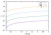 |
Fig. 1 Stopping time at the beginning of the simulation for the different particle sizes modelled. |
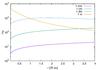 |
Fig. 2 Radial drift velocity profile at the equilibrium for the different particle sizes modelled. |
The transition between the Epstein and Stokes regimes is clearly visible in Fig. 2 where the radial drift velocity at equilibrium is plotted for the different particle sizes in the whole domain. As the particles approach a stopping time of order unity their radial velocity grows, so the highest value is associated with the dm particles in the outer disk and the m-sized particles in the inner parts. Furthermore, owing to the transition between the two drag regimes, the profile of the curves rapidly changes from cm- to m-sized particles. We note that when the planet starts to clear a gap, the gas surface density inside it drops, and thus the stopping time of particles in horseshoe orbit can increase up to 2 orders of magnitude (Paardekooper & Mellema 2006). The transition between the different drag regimes is then expected not only in the inner part of the disk but also near the planet co-orbital regions.
4.3. Planets
We embed two equal-mass planets that orbit their parent star in circular orbits with semi-major axes a1 = 1 and a2 = 2. Their masses range from 1 Mth = 0.07 MJup to 10 Mth = 0.7 MJup. Mass accretion is not allowed, and the planets do not feel the disk, so their orbital parameters remain fixed during the whole simulation. The gravitational potential of the planets is modelled through a Plummer-type prescription, which takes into account the vertical extent of the disk and avoids the numerical problems related to a point-mass potential. We used a smoothing value of ϵ = 0.6 H as this describes the vertically averaged forces very well (Müller et al. 2012). To prevent strong shock waves in the initial phase of the simulations, the planetary core mass is increased slowly over 20 orbits. Table 1 summarises the parameters of the standard model. With these values the gaps are not expected to overlap, even for the highest mass planet, because from Eq. (5) we have xs ≃ 0.18, thus  (26)The simulations were run for 600 orbital times of the inner planet, which corresponds to ~200 orbits of the outer planet, i.e. to ~105 yr, which is a consistent amount of time for a planetary system around a young star like HL Tauri which is only 106 yrold.
Models.
5. Results
5.1. Massive core (10 Mth)
Based on the criteria of gap opening reviewed in Sect. 2, two 10 Mth planets should rapidly open up a gap in the gas and dust disk. We study in detail the disk evolution for these massive cores; we focus on particle concentration, which happen mainly at gap edges.
In the following analysis the region of high surface density between the two planets is referred to as the ring. It will have an inner and outer edge, which correspond to the outer edge of the inner gap and the inner edge of the outer gap, respectively. Furthermore, there will be the outer edge of the outer gap and the inner edge of the inner gap. The study of the various gap edges, where there is an abrupt change in the surface density profile, is important since they are potentially unstable regions where gas and particles could collect, thus changing the final surface density distribution of the disk.
5.1.1. Gas distribution
The inner planet has already opened a clear gap after 100 orbits (Fig. 3, top panel) where, as expected by the general criterion of Crida et al. (2006), the surface density is an order of magnitude lower than its unperturbed value. Meanwhile, the outer planet is still opening its gap since it has a longer dynamical timescale.
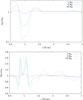 |
Fig. 3 Gas surface density (top panel) and vorticity profile (bottom panel) after 100 orbits. |
The steep profile in the surface density close to the ring’s inner edge can trigger a Rossby wave instability (RWI, Li et al. 2001). This instability gives rise to a growing non-axisymmetric perturbation consisting of anticyclonic vortices. A vortex is able to collect a high mass fraction and it can significantly change the final distribution of gas and dust in the disk. An important parameter to study when considering the evolution of vortices is the gas vorticity, which is defined as  (27)We show its profile in Fig. 3 (bottom panel) and its 2D distribution in Fig. 4 (bottom panel). Comparing the 2D distributions of vorticity and surface density (Fig. 4), we see that vorticity peaks where the gap is deeper, and low vorticity regions appear at the centre of spiral arms created by the planets and close to the ring’s inner edge.
The development of vortices due to the presence of a planet has been studied extensively. However, their evolution in a multiplanet system has not yet been addressed. From Fig. 4 we see that the outer planet substantially perturbs the co-orbital region of the inner one. There are two competing factors that need to be taken into account to estimate the lifetime of a vortex. On the one hand vortex formation is promoted by the enhanced surface density gradient at the ring location due to the combined action of both planets that push away the disk from their location. On the other hand, the periodic close encounters of the outer planet with the vortices enhance the eccentricity of the dust particles trapped in it, favouring their escape and thus depleting the solid concentration inside the vortex.
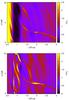 |
Fig. 4 Gas surface density (top panel) and vorticity distribution (bottom panel) at the end of the simulation for the massive cores case. |
The capacity of particles collected by a vortex is closely linked to its orbital speed. If a vortex has a Keplerian orbital speed, then dust particles with the same orbital frequency will remain in the vortex for many orbits and slowly drift to its centre as a result of the drag forces. On the other hand, a particle in a vortex orbiting with a non-Keplerian frequency will experience a Coriolis force in the Keplerian reference frame and, if the drag force is unable to counteract it, the particle will leave the vortex (Youdin 2010).
The evolution of vortices can be also studied from the dynamics of coupled particles, which closely follow the gas dynamics. From the analysis of cm-sized particles near the ring’s inner edge (Fig. 5), we can see that after 50 orbits two vortices are already visible and they last for several tens of orbits. The outer planet stretches the vortices periodically, and as a result they slowly shrink in size.
In order to see if the vortices that develop in our simulation are capable of collecting a large fraction of particles, in Fig. 5 we plot the vortices in a co-moving frame with the disk at r = 1.3. The two vortices follow the Keplerian speed within a few percentage points, thus they are potentially able to trap a consistent fraction of particles.
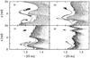 |
Fig. 5 Distribution of cm-sized particles at different time steps (50, 60, 70, 80 orbital times) at the ring’s inner edge for the massive cores case. The evolution of two vortices in a frame co-moving with the disk at 1.3 au is shown. The vortex centre orbits the central star with a velocity close to the background Keplerian speed, which promotes particle trapping inside the vortex. |
The influence of the outer planet on the development of RWI at the gap edge is studied by running a different model with only one massive planet (M = 10 Mth) at r = 1.0 (Fig. 6). The particle concentration near the inner ring is weaker in the single core simulation. As a result, the vortices that form are less prominent and their lifetime is shorter, even though the perturbation to the ring’s inner edge is smaller than in the dual core simulation.
 |
Fig. 7 Dust normalised surface density distribution for the m- (first panel), dm- (second panel), cm- (third panel), and mm-sized (fourth panel) particles disk and two equal-mass 10 Mth cores at r = 1,2 at four different times (50, 100, 300, 600 orbital times) for each case. |
5.1.2. Particle distribution
The evolution of the normalised surface density of the various dust species is shown in Fig. 7. The inner and outer planets rapidly carve (the first 50 orbits) a particle gap, except for the most coupled particles simulated (mm-sized), which are cleared on a longer timescale for the outer planet (see Fig. 7, fourth panel). As stated before, this behaviour is only due to the longer dynamical timescale of the outer planet, and it closely follows the evolution of the gas in the outer gap.
A significant fraction of particles clump in the co-orbital region with the inner planet for several hundred periods. However, they are finally disrupted by the tidal interaction with the outer planet which excite their eccentricities, causing a close fly-by with the inner planet. The only particles that remain for the whole simulated period in the co-orbital region are the m-sized ones, even though they are perturbed and a significant mass exchange between the two Lagrangian points (L4 and L5) takes place (see Fig. 7, first panel and Fig. 8, bottom right panel). The outer planet is also able to keep a fraction of particles in the co-orbital region for longer timescale, though they are much more dispersed than the Lagrangian points. Moreover, in all simulations the L4 Lagrangian point is the most populated.
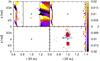 |
Fig. 8 Particle distribution near the inner massive planetary core location for mm- (top left), cm- (top right), dm- (bottom left), and m-sized (bottom right) particles at the end of the simulation. The velocity vectors of the particles with respect to the planet are shown and the colour scale highlights the radial velocity component. |
The ring, which forms between the two gaps, quickly becomes very narrow and it stabilises in a position close to the 5:3 mean motion resonance (MMR) with the inner planet that seems to be a stable orbit. As shown in Fig. 9, the particles in the ring clump around five symmetric points which gain a high mass.
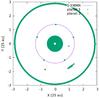 |
Fig. 9 Distribution of dm-sized particles at the end of the simulation of the two massive cores. The particle ring between the two planets shrinks with time until it clumps in a few stable points that form a pentagon-like structure with an orbit close to the 5:3 MMR with the inner planet at r = 1.4. |
There are visible vortices in the particle distribution in the first hundred orbits for the cm-sized particles at the inner ring edge (third panel). Although these structures are prominent in the particle distribution of cm-sized dust, they are not visible in the other dust size distributions mainly because the ring quickly becomes very narrow for larger particles and so there is no time for them to be trapped in the vortex.
The velocity components of the particles shown in Fig. 8 highlight the strong perturbations due to the spiral arm generated by the outer planet which mainly affects the most coupled particles and the gas. The bodies passing close to the planet location, as in the meter case shown in Fig. 8 (bottom right panel), gain a high velocity component that is represented by the long black arrow.
Finally, the particle distributions at the end of the simulation (see Fig. 8) show the dependence of gap width on particle size. The mm-sized particles (Fig. 8, top left panel) reach a region closer to the planet where we overplot the minimum half-gap width as calculated from Eq. (5), showing that the dynamics of the smallest particles closely follow that of the gas. The other particles have increasingly larger gaps. The dm-sized particles (Fig. 8, bottom left panel) have almost completely cleared the gap region since they have a stopping time closer to one near the planet’s location and thus their evolution is faster.
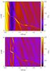 |
Fig. 10 Gas surface density (top panel) and vorticity distribution (bottom panel) at the end of the intermediate mass cores simulation. |
5.2. Intermediate mass core (5 Mth)
The intermediate mass planet should still open up a gap in the gaseous disk, but on a much longer timescale, since from Eq. (3) the opening timescales is q-2.
5.2.1. Gas distribution
From the density profile of Fig. 3 (first panel) we can see that after 100 orbits there is a visible gap opened by the inner planet, even if it is considerably shallower than the massive cores case, as it is for the vorticity profile (second panel). The outer planet still perturbs the co-orbital region of the inner one (Fig. 10), but its magnitude is reduced and it has barely modified the unperturbed surface density distribution at its location.
Even though the influence of the outer planet is less dramatic than the more massive case, the reduction of the steepness of the surface density profile hinders the development of vortices near the ring’s inner edge.
5.2.2. Particle distribution
The intermediate mass inner planet carves a gap in the dust disk after 50 orbits for all the particle sizes (Fig. 11). Instead, after 50 orbits the outer planet is able to clean its gap only for the most decoupled particles (dm and m), while it takes 300 orbits to clean a gap in the cm particles (third panel), and it has only opened a partial gap in the mm-sized particles disk at the end of the simulation (fourth panel). The dm particles (second panel) have the highest migration speed in the outer disk, as expected from Fig. 2, and after 300 orbits they are all distributed in narrow regions at the gap edges and in co-orbital region with the outer planet. On the other hand, the cm particles (third panel) are more coupled to the gas and the outer planet has not yet carved a gap that is able to confine them in the outer regions of the disk at the end of the simulation. Thus, after 600 orbits we observe that they engulf the planet gap (third panel, last screenshot).
The dependence of the gap width on particle size is highlighted in Fig. 12 where we can see a strong difference between the mm particle gap, which follows the gas dynamic and remains close to the location of the half-gap width (xs) overplotted on the first panel and the gap width of the other particles.
The interaction between the two planets on the long term disrupts the particles clumping around the stable Lagrangian points, as in the more massive case. At the end of the simulation only the m and mm particles (Fig. 12) are still present in the co-orbital region, preferably at the L5 point.
The clumping of particles in few stable points at the ring location is still visible in the intermediate mass case, but only in the m, and dm cases (first and second panels of Fig. 11). Furthermore, some vortices form in the outer part of the particle disk of cm dust (third panel of Fig. 11). However, they are numerical artefacts because the disk’s outer edge is initialised with a sharp density profile cut, which in the long term favours the development of vortices.
 |
Fig. 11 Dust normalised surface density distribution for the m- (first panel), dm- (second panel), cm- (third panel), and mm-sized (fourth panel) particles disk and two equal-mass 5 Mth cores at r = 1,2 at four different times (50, 100, 300, 600 orbital times) for each case. |
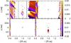 |
Fig. 12 Particle distribution near the inner intermediate mass planetary core location for mm- (top left), cm- (top right), dm- (bottom left) and m-sized (bottom right) particles at the end of the simulation. The velocity vectors of the particles with respect to the planet are shown and the colour scale shows the relative radial velocity. |
5.3. Low mass core (1 Mth)
Finally, we explore the low mass core scenario in order to study a case where the particle ring between the two planets does not clump into a few stable points and the gaps carved by planets remain narrow, as is seen in the HL Tau system.
5.3.1. Gas distribution
Figure 3 (top panel) shows that both the inner and outer planets are not massive enough to clear a gap in the gaseous disk within the simulated time. From the 2D distribution of the surface density and vorticity (Fig. 13) it is possible to see that the presence of the two planets slightly changes the unperturbed state of the gaseous disk (where the scale has been changed with respect to the plots of the more massive cases in order to highlight the small differences).
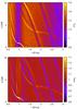 |
Fig. 13 Gas surface density (top panel) and vorticity distribution (bottom panel) at the end of the simulation for the two low mass cores. |
5.3.2. Particle distribution
Although the gas profile is not changed considerably owing to the small mass of the planets, they are able to open up clear gaps in the dust disk in the first 50 orbits for m- and dm-sized particles (Fig. 14), while it takes 100 orbits for the cm-sized particles and at the end of the simulation it is still clearing the gap for most of the coupled particles. As stated before, this process takes longer for the outer planet, which is able to open a clear gap only at the end of the simulation for all but the mm-sized particles where only a partial gap is barely visible.
 |
Fig. 14 Dust normalised surface density distribution for the m- (first panel), dm- (second panel), cm- (third panel), and mm-sized (fourth panel) particles disk and two equal-mass 1 Mth cores at r = 1,2 at four different times (50, 100, 300, 600 orbital times) for each case. |
A significant fraction of particles remains in the co-orbital region with both the inner and outer planet for the whole period simulated. As found for the massive core case, their density is higher at the L4 point. Also in this case, the dm size particles are the ones with the fastest dynamical evolution and it is possible to see in Fig. 14 (third panel) that after 300 orbits the outer disk engulfs the outer planet’s co-orbital region, which is unable to filtrate those particles effectively. In this case, the ring between the two planets does not clump in a small number of stable points; it remains wide for the whole simulation, though it shrinks with time and its width depends on the particle size (Fig. 15, top panel).
From Fig. 14 (first panel) it is also possible to see the formation of ripples just outside the location of the outer planet. This effect can be seen also from the final eccentricity distribution of the m-sized particles (Fig. 15, bottom panel). This behaviour is due to the eccentricity excitation of particles that passes close to the planet’s location. For less coupled particles, the interaction with the gas takes several orbital time steps to smooth out the eccentricity, thus these typical structures form. This effect is only visible in the low mass cores simulation since the particle gap is narrower, thus the particles get closer to the planet and the excitation of their eccentricity is higher.
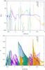 |
Fig. 15 Particle surface density (top panel) and eccentricity profile (bottom panel) at the end of the simulation for the different particle species. |
In Fig. 16 we focused on the gap structure close to the inner planet location for the different particle sizes at the end of the simulation. We also overplot the minimum gap half-width xs to test whether this condition is met for the most coupled particles that follow the gas dynamics. From the distribution of mm-sized particles we can see that the gap is opened exactly at the location of the minimum gap half-width, and there is still a lot of material in the horseshoe region. The gap is considerably wider for the cm-sized particles.
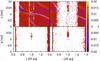 |
Fig. 16 Particle distribution near the inner low mass planetary core location for mm- (top left), cm- (top right), dm- (bottom left), and m-sized (bottom right) particles at the end of the simulation. The velocity vectors of the particles with respect to the planet are shown and the colour scale shows the relative radial velocity. |
Finally, in Fig. 17 we highlight the constant mass transfer that take place through the inner planet location for the most coupled particles that are not effectively filtered by the less massive planet. We plot the radial velocity of the particles with a colour scale to emphasise the flow in both directions.
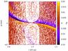 |
Fig. 17 Mass transfer through the planet position of mm-sized particles for the 1 thermal mass planet, which is unable to effectively filtrate them. The particles are plotted together with their velocity vectors and the colour scale indicates their radial velocities. |
6. Discussion
6.1. Path to a second generation of planets
The possibility of creating the conditions for a second generation of planets by a massive core has already been studied in the past. However, the combined action of a multiplanetary system can achieve the same goal from less massive first generation planets. As we show in Sect. 5.1, two 10 Mth = 0.7 MJup can trigger vortex formation which are more prominent and live longer than the single mass case. However, these vortices appear to be a transient effect; they develop after more than 80 orbits of the inner planet and last until 120 orbits, thus it is difficult to relate this behaviour to an initial condition effect and it does not depend on the timescale over which the planets are grown in the simulation. Furthermore, vortex formation depends on viscosity and can persist for longer times in low viscosity disks. Although the main dust collection driver is the ring generated by the combined action of the two planets, vortices can create some characteristic observable features, locally enhancing the dust surface density. Moreover, for both the massive and intermediate mass cores, the particle ring clumps into a few symmetric points close to the 5:3 MMR which are stable for several hundred orbits. Taking a dust-to-gas mass ratio of 0.01, we found that the mass collected in these stable points can reach several Earth masses. However, we note that this strong mass clumping might be reduced by the introduction of particle diffusion due to disk turbulence.
6.2. Comparison with previous work
This is one of the first studies on dust evolution and filtration in a multiple planet system, thus there is no direct comparison with similar setups. However, recently Zhu et al. (2014) have performed an extensive analysis of the dust filtration by a single planet in a 2D and 3D disk from which we have taken some ideas and so is the natural test comparison for the different outcomes of our analysis.
One first interesting comparison between the two results is the possibility of forming vortices at the gap edges, taking into account that in the Zhu et al. (2014) scenario vortex development was favoured by the choice of a non-viscous disk. Even if for a single planet the vortices are hindered, we found that the presence of an additional planet can enhance the density at the ring location and can promote the development of vortices. Moreover, we obtain the ripple formation again as in Zhu et al. (2014) for decoupled particles close to the planet location.
Zhu et al. (2014) also found a direct proportionality between the gap width and the planet mass, where a 9 MJup induced a vortex at the gap edge at a distance more than twice the planet’s semi-major axis. Although we have not modelled such high mass planets we did obtain a similar outcome for our parameter space.
In our simulation we do not find the presence of strong MMR that aids the gap clearing since we do not model particles with stopping times greater than ~5, thus the coupling with the gas disrupts the MMR . They become important only when the gas surface density is highly depleted, such as in the ring between planets for the high mass cases, where a 5:3 MMR with the inner planet is found to be a stable location.
Furthermore, as observed in Ayliffe et al. (2012) there is a strong correlation between particle size and particle gap, where the most coupled particles reach regions closer to the planet and can be accreted by the planet or can migrate to the inner disk, while less coupled particles are effectively filtrated by the planet.
6.3. Comparison with observations
Pre-transitional disks are defined observationally as disks with gaps. These features are observed in many cases in the sub-mm dust emission and there is no evidence that the gaseous emission follows the same pattern. The observation of transitional and pre-transitional disks highlights different physical behaviours that need to be explained. A major problem is the coexistence of a significant accretion rate onto the star (up to the same order as common T Tauri stars, CTTS) with dust cleared zones, and the absence of near-infrared (NIR) emission. One of the most plausible explanations is the presence of multiple giant planets that can create a common gap and thus enhance the accretion rate across them, exchanging torque with the disk while depleting the dust component through a filtration mechanism that, together with dust growth, can explain the absence of a strong NIR emission in (pre-)transitional disks compared to full disks (Zhu et al. 2012). For a full review of the topic see Espaillat et al. (2014).
In the HL Tau system, although several rings have been observed in its dust emission, it still has a very high accretion rate onto the star Ṁ = 2.13 × 10⁻⁶M⊙/yr (Robitaille et al. 2007). This is proof that, at least in this system, the rings observed in the dust emission are not related to rings in the gas distribution.
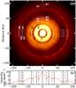 |
Fig. 18 Top panel: deprojected image from the mm continuum of HL Tau. Bottom panel: cross-cuts at PA = 138° through the peak of the mm continuum of HL Tau ALMA Partnership et al. (2015). |
Since we found that a wide ring is observed in our simulations only for the small mass case and that a clear gap is visible for the outer planet only in the intermediate and massive core cases, we choose to run a different model with an inner small mass core and an outer intermediate mass core in order to compare the outcome of our simulations with the HL Tau system. We rescaled the system and ran a different simulation to compare it to the real one, placing the inner planet at 32.3 au corresponding to the D2 gap (see Fig. 18, top panel) and the outer one at 64.6 au, keeping the 2:1 ratio, which is close to the location of B5. Comparing the 2D surface density distribution at the end of the simulation with the deprojected image in the continuum emission and their slices (Figs. 18, 19) we can outline several shared features and differences. The gap created by the inner planet has a very similar configuration to the one observed. On the other hand there are no clear visible features inside its orbit in the observed image, while a variety of inner structures are visible in the output of the simulation. These features are mainly due to the inner wave generated by the planet. The strong gap that is visible close to the star is instead not physical and is related to the inner boundary condition. In the outer part of the disk, several differences can be noted. The most important is the high surface density in the horseshoe region, which is related to our choice of an initial flat profile for the particle distribution. Although this approximation was chosen to extend the simulated time in order to prevent a fast depletion of material from the outer disk, it also favoured the dust trapping by the outer planet. Moreover, the particle ring is more depleted than in the observed image. Thus, we expect that the planetary mass responsible for the observed outer gap should be slightly smaller than the one adopted in this simulation. We also note the strong depletion of dust particles just inside the outer planet location due to its dust filtration mechanism, which is clear from the bottom panel of Figure 18. Because of this effect, in a multiplanetary system a planet is not necessary located where the gap is deeper, but it could be at the rim of the gap preventing the particles of a certain size from crossing its location.
However, except for these differences given by our initial choice of the parameter space, the structures obtained from the simulations are similar to what is observed.
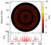 |
Fig. 19 Top panel: final mm-dust surface density distribution for an inner low mass core and an outer intermediate mass core. Bottom panel: relative surface density distribution. |
6.4. Dependence on the disk surface density
The dynamical evolution of dust particles is closely linked to their stopping time, which is directly related to the disk surface density through Eq. (20), for the Epstein regime. Thus, if we decrease the disk surface density by a factor of 10 in order to stabilise the disk in the isothermal case (see Appendix A for a study of the disk stability with a more realistic equation of state), we need to lower the particle size by the same factor to reobtain the same particle dynamics. On the other hand, if we want to keep the particle’s size fixed, so that we can compare our results with the ALMA continuum images, we need to decrease the planetary mass since the gap width depends on the particle stopping time. We tried a different choice of the parameter space to obtain a similar output with a much smaller disk mass and planetary mass cores. In Fig. 20 we show a run with a disk mass of 1/10 of the test case. The width of the gap created by two planets is similar, as outlined in the bottom panel. However, in this case the planetary mass adopted to open such narrow gaps in the particle disk are much lower: ~10 and ~20 M⊕ for the inner and outer planet, respectively. These lower values of the planetary masses prove that the ability of planets to open gaps in the dust disk is widely applicable, and increases the likelihood of the planetary origin through core accretion in this young system at large radii (~60 au). It will be crucial to define the disk mass more accurately in order to constrain the particle dynamics and the planetary mass growing inside their birth disk.
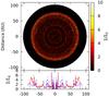 |
Fig. 20 Top panel: dust distribution for the mm-sized particles disk and two planetary cores of ~10 and ~20 M⊕ after 250 orbits of the inner planet. Bottom panel: relative surface density distribution (red solid curve) where the distribution of the higher disk mass case (from Fig. 19 has been overplotted (blue dashed curve). |
7. Conclusion
We implemented a population of dust particles into the 2D hydro code fargo (Masset 2000) to study the coupled dynamic of dust and gas. The dust is modelled through Lagrangian particles, which permits us to cover the evolution of both small dust grains and large bodies within the same framework. In particular we studied dust filtration in a multiplanetary system to obtain some observable features that can be used to interpret the observations made by modern infrared facilities like ALMA . From the analysis of our simulations we have found that the outer planet
-
affects the co-orbital region of the inner one exciting the particlesin the Lagrangian points (L4 and L5), which are effectivelyremoved in the majority of the cases;
-
increases the surface density in the region between them, creating a particle ring that can clump into a small number of symmetric points, collecting a mass up to several Earth masses;
-
promotes the development of vortices at the ring’s inner edge, increasing the steepness of the surface density profile.
Moreover, when the planets are not massive enough to create a narrow particle ring between the planets, its width depends on the particle size. This could be a potentially observable feature that can link the ring formation with the presence of planets. Furthermore, we confirmed previous results regarding the particle gap, which develops much more quickly than the gaseous one, and is wider for higher mass planets and more decoupled particles.
The features observed in the HL Tau system can be explained by the presence of several massive cores, or lower mass cores depending on the adopted surface density, that shape the dust disk. We find that the inner planet(s) should be of the order of 1 Mth = 0.07 MJup to open a small gap in the dust disk while keeping a wide particle ring. The outer one(s) should have a mass of the order of 5 Mth = 0.35 MJup to open a visible gap. These values are in agreement with those found by Kanagawa et al. (2015), Dipierro et al. (2015), Dong et al. (2015). We note that decreasing the disk surface density by a factor of 10 reduces the planetary mass needed to open the observed gaps to a value of 10 M⊕ and 20 M⊕ for the inner and outer planets, respectively. These reduced values render the planet formation through core accretion more reliably in the young HL Tau system. Although the particle gaps observed are prominent, the expected gaseous gaps would be barely visible.
The limitations of this work are the lack of particle back-reaction on the gas, self-gravity of the disk, and particle diffusion. Furthermore, we did not model the accretion of particles onto the planet and planet migration. These approximation were chosen in order to study the global evolution of particle distribution with different stopping times and different planet masses, without increasing excessively the computation time. Although the disk is very massive, the asymmetric features typical of a gravitationally unstable disk are not observed in the continuum mm observations that should correctly describe the gas flow, thus we do not expect the real system to be subject to strong perturbations due to its self-gravity. The particle-back reaction plays an important factor when studying the evolution of particle clumps, but it is not expected to change the global dust distribution significantly. However, particle diffusion could have an important role both in reducing the dust migration and in preventing strong clumping of particles. We are planning to relax these approximations in future works, and to run more accurate simulations and test the contribution of the individual physical process on the final dust filtration and distribution. Moreover, we limited our analysis to the peculiar case of equal-mass planets on a fixed orbit, and changing each one of these conditions can result in a very different outcome. The possibility of evolving the simulations further in time was considered since the outer planets were not able to open up a clear gap for the less massive cases. However, in all cases they are able to open only a very shallow gap, so the possible influence on the subsequent evolution of the particles close to their position is not expected to be significant. Furthermore, since we modelled the system for ~105 yr around a young star (~106 yr), and we needed to form the planetary cores in the first place, it does not seem unrealistic to observe a planet at ~60 au that is still in the gap clearing phase.
Acknowledgments
We thank an anonymous referee for his useful comments and suggestions. G. Picogna acknowledges the support through the German Research Foundation (DFG) grant KL 650/21 within the collaborative research program “The first 10 Million Years of the Solar System”. Some simulations were performed on the bwGRiD cluster in Tübingen, which is funded by the Ministry for Education and Research of Germany and the Ministry for Science, Research and Arts of the state Baden-Württemberg, and the cluster of the Forschergruppe FOR 759 “The Formation of Planets: The Critical First Growth Phase” funded by the DFG.
References
- ALMA Partnership, Brogan, C. L., Pérez, L. M., et al. 2015, ApJ, 808, L3 [NASA ADS] [CrossRef] [Google Scholar]
- Armitage, P. J. 2010, Astrophysics of Planet Formation (Cambridge University Press) [Google Scholar]
- Ayliffe, B. A., Laibe, G., Price, D. J., & Bate, M. R. 2012, MNRAS, 423, 1450 [NASA ADS] [CrossRef] [Google Scholar]
- Bai, X.-N., & Stone, J. M. 2010, ApJSS, 190, 297 [NASA ADS] [CrossRef] [Google Scholar]
- Baruteau, C., & Masset, F. S. 2008, AJ, 672, 1054 [Google Scholar]
- Crida, A., Morbidelli, A., & Masset, F. S. 2006, Icarus, 181, 587 [Google Scholar]
- de Val-Borro, M., Edgar, R. G., Artymowicz, P., et al. 2006, MNRAS, 370, 529 [NASA ADS] [CrossRef] [Google Scholar]
- Dipierro, G., Price, D., Laibe, G., et al. 2015, MNRAS, 453, L73 [NASA ADS] [CrossRef] [Google Scholar]
- Dong, R., Zhu, Z., & Whitney, B. 2015, ApJ, 809, 93 [NASA ADS] [CrossRef] [Google Scholar]
- Epstein, P. S. 1924, Phys. Rev., 23, 710 [NASA ADS] [CrossRef] [Google Scholar]
- Espaillat, C., Muzerolle, J., Najita, J., et al. 2014, Protostars and Planets VI, 497 [Google Scholar]
- Flock, M., Ruge, J. P., Dzyurkevich, N., et al. 2015, A&A, 574, A68 [NASA ADS] [CrossRef] [EDP Sciences] [Google Scholar]
- Fouchet, L., Maddison, S. T., & Murray, J. R. 2007, A&A, 474, 1037 [NASA ADS] [CrossRef] [EDP Sciences] [Google Scholar]
- Haghighipour, N., & Boss, A. P. 2003, AJ, 583, 996 [Google Scholar]
- Kanagawa, K. D., Muto, T., Tanaka, H., et al. 2015, ApJ, 806, L15 [NASA ADS] [CrossRef] [Google Scholar]
- Korycansky, D. G., & Papaloizou, J. C. B. 1996, ApJSS, 105, 181 [NASA ADS] [CrossRef] [Google Scholar]
- Kwon, W., Looney, L. W., & Mundy, L. G. 2011, ApJ, 741, 3 [NASA ADS] [CrossRef] [Google Scholar]
- Landau, L. D., & Lifshitz, E. M. 1959, Fluid mechanics (Pergamon Press) [Google Scholar]
- Li, H., Colgate, S. A., Wendroff, B., & Liska, R. 2001, ApJ, 551, 874 [NASA ADS] [CrossRef] [Google Scholar]
- Lin, D. N. C., & Papaloizou, J. C. B. 1979, MNRAS, 186, 799 [NASA ADS] [CrossRef] [Google Scholar]
- Lin, D. N. C., & Papaloizou, J. C. B. 1986, ApJ, 309, 846 [NASA ADS] [CrossRef] [Google Scholar]
- Lin, D. N. C., & Papaloizou, J. C. B. 1993, in Protostars and Planets III, eds. E. H. Levy, & J. I. Lunine (University of Arizona Press), 749 [Google Scholar]
- Masset, F. S. 2000, A&AS, 141, 165 [NASA ADS] [CrossRef] [EDP Sciences] [Google Scholar]
- Masset, F. S., D’Angelo, G., & Kley, W. 2006, ApJ, 652, 730 [NASA ADS] [CrossRef] [Google Scholar]
- Müller, T. W. A., Kley, W., & Meru, F. 2012, A&A, 541, A123 [NASA ADS] [CrossRef] [EDP Sciences] [Google Scholar]
- Nakagawa, Y., Sekiya, M., & Hayashi, C. 1986, Icarus, 67, 375 [NASA ADS] [CrossRef] [Google Scholar]
- Paardekooper, S.-J. 2007, A&A, 462, 355 [NASA ADS] [CrossRef] [EDP Sciences] [Google Scholar]
- Paardekooper, S.-J., & Mellema, G. 2004, A&A, 425, L9 [NASA ADS] [CrossRef] [EDP Sciences] [Google Scholar]
- Paardekooper, S.-J., & Mellema, G. 2006, A&A, 453, 1129 [NASA ADS] [CrossRef] [EDP Sciences] [Google Scholar]
- Papaloizou, J. C. B., & Lin, D. N. C. 1984, ApJ, 285, 818 [NASA ADS] [CrossRef] [Google Scholar]
- Papaloizou, J. C. B., & Terquem, C. 2006, Rep. Progr. Phys., 69, 119 [NASA ADS] [CrossRef] [Google Scholar]
- Robitaille, T. P., Whitney, B. A., Indebetouw, R., & Wood, K. 2007, ApJS, 169, 328 [NASA ADS] [CrossRef] [Google Scholar]
- Supulver, K. D., & Lin, D. N. C. 2000, Icarus, 146, 525 [NASA ADS] [CrossRef] [Google Scholar]
- Weidenschilling, S. J. 1977, MNRAS, 180, 57 [NASA ADS] [CrossRef] [Google Scholar]
- Whipple, F. L. 1972, in From Plasma to Planet, ed. A. Elvius (Stockholm: Wiley), 211 [Google Scholar]
- Youdin, A. N. 2010, in Physics and Astrophysics of Planetary Systems, eds. T. Montmerle, D. Ehrenreich, & A.-M. Lagrange, EAS Publ. Ser., 41, 187 [Google Scholar]
- Zhang, K., Blake, G. A., & Bergin, E. A. 2015, ApJ, 806, L7 [NASA ADS] [CrossRef] [Google Scholar]
- Zhu, Z., Nelson, R. P., Dong, R., Espaillat, C., & Hartmann, L. 2012, ApJ, 755, 6 [NASA ADS] [CrossRef] [Google Scholar]
- Zhu, Z., Stone, J. M., Rafikov, R. R., & Bai, X.-N. 2014, ApJ, 785, 122 [NASA ADS] [CrossRef] [Google Scholar]
Appendix A: Disk stability
The disk parameters adopted in this work were selected to match the observational data (Kwon et al. 2011). We point out that the disk-to-star mass ratio is relatively high and, in the locally isothermal approximation, it is gravitationally unstable in the outer regions considering its Toomre parameter 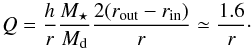 (A.1)However, the isothermal equation of state is usually a poor representation of the temperature distribution in the disk, especially for the inner regions of protoplanetary disks around young stars. To validate this model we ran an additional hydro simulation in which we include a more realistic equation of state where the radiative transport and radiative cooling are included. From Fig. A.1 it is clear that the more appropriate equation of state prevents the disk from becoming even partially unstable. The different equation of state could in principle affect the gap opening timescale; however, the long term evolution of the particle dynamics is not expected to vary significantly. Moreover, the important parameter in our study is the stopping time of the particles, so the results obtained remain valid for different values of the surface density profile, scaling accordingly the dust size, as discussed in Sect. 6.4.
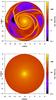 |
Fig. A.1 Disk surface density after 20 inner planetary orbits for the isothermal case (top panel) and fully radiative case (bottom panel) where the self-gravity of the disk is considered. |
Appendix B: Integrators
In order to model the dynamics of the particle population in our simulations we tried different integrators.
Appendix B.1: Semi-implicit integrator in polar coordinates
To follow the dynamics of particles that are well-coupled with the gas and that have a stopping time much smaller than the time step adopted to evolve the gas dynamics, we adopted the semi-implicit leapfrog (drift-kick-drift) integrator described in Zhu et al. (2014) in polar coordinates. This method guarantees the conservation of the physical quantities for the long term simulations performed in this paper, and at the same time it is faster than an explicit method.
Scheme
Half Drift:
![Mathematical equation: \appendix \setcounter{section}{2} \begin{eqnarray} && v_{{R},n+1} = v_{{R},n} \\[1.5mm] && l_{n+1} = l_n \\[1.5mm] && R_{n+1} = R_n + v_{{R},n}\frac{\mathrm{d}t}{2} \\[1.5mm] && \phi_{n+1} = \phi_{n}+\frac{1}{2}\left( \frac{l_n}{R_n^2}+\frac{l_{n+1}} {R_{n+1}^2}\right) \frac{\mathrm{d}t}{2}; \end{eqnarray}](/articles/aa/full_html/2015/12/aa26921-15/aa26921-15-eq153.png) Kick:
Kick: ![Mathematical equation: \appendix \setcounter{section}{2} \begin{eqnarray} && R_{n+2} = R_{n+1} ~~~~~~~~~~~~~~~~~~~~~~~~~~~~~~~~~~~~~~~~~~~~~~~~~~~~~~~~~~~~~~~~~~~~~~~~~~~~~~~~~~~~~~~~~~~~~~~\\[1.5mm] && \phi_{n+2} = \phi_{n+1} \\[1.5mm] && l_{n+2} = l_{n+1} + \frac{{\rm d}t}{1+\frac{\mathrm{d}t}{2t_{\mathrm{s},n+1}}} \left[-{\left(\frac{\partial\Phi}{\partial\phi}\right)}_{n+1} + \frac{v_{\mathrm{g,\phi},n+1}R_{n+1}-l_{n+1}}{t_{\mathrm{s},n+1}} \right] \\[1.5mm] && v_{{R},n+2} = v_{{R},n+1} + \frac{{\rm d}t}{1+\frac{\mathrm{d}t}{2t_{\mathrm{s},n+1}}} \Bigg[ \frac{1}{2}\Bigg( \frac{l_{n+1}^2}{R_{n+1}^3}+ \frac{l_{n+2}^2}{R_{n+2}^3} \Bigg)- \Bigg( \frac{\partial\Phi}{\partial R} \Bigg)_{n+1} \\[1.5mm] & &\qquad\qquad +~\frac{v_{\mathrm{g,R},n+1}-v_{{R},n+1}} {t_{\mathrm{s},n+1}} \Bigg]; \end{eqnarray}](/articles/aa/full_html/2015/12/aa26921-15/aa26921-15-eq154.png) Half Drift:
Half Drift: ![Mathematical equation: \appendix \setcounter{section}{2} \begin{eqnarray} && v_{{R},n+3} = v_{{R},n+2} \\[1.5mm] && l_{n+3} = l_{n+2} \\[1.5mm] && R_{n+3} = R_{n+2} + v_{{R},n+3}\frac{\mathrm{d}t}{2} \\[1.5mm] && \phi_{n+3} = \phi_{n+2}+\frac{1}{2}\left( \frac{l_{n+2}}{R_{n+2}^2}+\frac{l_{n+3}} {R_{n+3}^2}\right) \frac{\mathrm{d}t}{2}; \end{eqnarray}](/articles/aa/full_html/2015/12/aa26921-15/aa26921-15-eq155.png) where vR is the radial velocity, l the angular momentum, R the cylindrical radius, and φ the polar angular coordinate. The index n shows the step at which the various quantities are considered. Further information regarding to the integrator can be found in Zhu et al. (2014).
where vR is the radial velocity, l the angular momentum, R the cylindrical radius, and φ the polar angular coordinate. The index n shows the step at which the various quantities are considered. Further information regarding to the integrator can be found in Zhu et al. (2014).
Appendix B.2: Fully-implicit integrator in polar coordinates
For particles with stopping times much smaller than the numerical time step, the drag term can dominate the gravitational force term, causing the numerical instability of the integrator. Thus, it is necessary to adopt a fully implicit integrator following Bai & Stone (2010), Zhu et al. (2014)
Scheme
Predictor step: ![Mathematical equation: \appendix \setcounter{section}{2} \begin{eqnarray} && R_{n+1} = R_n + v_{{R},n} \mathrm{d}t \\[2mm] && \phi_{n+1} = \phi_n+\frac{l_n}{R_n^2} \mathrm{d}t; \end{eqnarray}](/articles/aa/full_html/2015/12/aa26921-15/aa26921-15-eq161.png) Shift:
Shift: ![Mathematical equation: \appendix \setcounter{section}{2} \begin{eqnarray} && v_{{R},n+1} = v_{{R},n} + \frac{{\diff t}/2} {1+\diff t{\left( \frac{1}{2t_{\mathrm{s},n}} + \frac{1}{2t_{\mathrm{s},n+1}} + \frac{\diff t}{2t_{\mathrm{s},n}t_{\mathrm{s},n+1}} \right)}} \nonumber\\ & &\qquad \qquad \times~ \Bigg[ -{\left(\frac{\partial\Phi}{\partial R}\right)}_n -\frac{v_{{R},n}-v_{\mathrm{g,R},n}}{t_{\mathrm{s},n}} +\frac{l_n^2}{R_n^3} + \Bigg( -{\left(\frac{\partial\Phi}{\partial R}\right)}_{n+1} \nonumber \\ & &\qquad \qquad -~\frac{v_{{R},n}- v_{\mathrm{g,R},n+1}}{t_{\mathrm{s},n+1}} +\frac{l_{n+1}^2}{R_{n+1}^3} \Bigg) {\left(1+\frac{\diff t}{t_{\mathrm{s},n}}\right)} \Bigg] ; \\ && l_{n+1} = l_{n} + \frac{{\diff t}/2} {1+\diff t\left(\frac{1}{2t_\mathrm{s,n}}+\frac{1} {2t_{\mathrm{s},n+1}}+ \frac{\diff t}{2t_{\mathrm{s},n}t_{\mathrm{s},n+1}}\right)} \nonumber \\ & &\qquad \quad \times~ \Bigg[ -{\left(\frac{\partial\Phi}{\partial \phi}\right)}_n -\frac{l_n - R_n v_{\mathrm{g,\phi},n}}{t_{\mathrm{s},n}} +\Bigg( -{\left(\frac{\partial\Phi}{\partial \phi} \right)}_{n+1} \nonumber \\ & &\qquad \quad -~\frac{l_n - R_{n+1} v_{\mathrm{g,\phi},n+1}} {t_{\mathrm{s},n+1}} \Bigg) {\left(1+\frac{\diff t}{t_{\mathrm{s},n}}\right)} \Bigg]; \end{eqnarray}](/articles/aa/full_html/2015/12/aa26921-15/aa26921-15-eq162.png) Corrector step:
Corrector step: 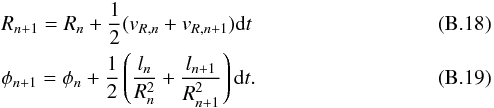
Appendix C: Particle tests
To test the numerical integrators described in Sect. B, we did an orbital test and the drift test proposed by Zhu et al. (2014).
Appendix C.1: Orbital tests
We release one dust particle at r = 1, φ = 0, with vφ = 0.7, and integrate it for 20 orbits. The time steps Δt are varied between 0.1 and 0.01 in units of the orbital time. The results are shown in Fig. C.1. The particle follows an eccentric orbit with e = 0.51. The time steps are Δt = 0.1, compared with the orbital time (2π). The precession observed occurs because even symplectic integrators cannot simultaneously preserve angular momentum and energy exactly. The advantage of the semi-implicit scheme is that it preserves geometric properties of the orbits, while the fully implicit integrator does not. For comparison, the orbit is also calculated with an explicit integrator, but with a much smaller time step Δt = 0.01, showing no visible precession. This behaviour is also found with the implicit schemes reducing the numerical time step. Since Δt = 0.01 is normally the time step used in our planet-disk simulations, our integrators are quite accurate even if we integrate the orbit of particles having moderate eccentricity.
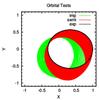 |
Fig. C.1 Orbital evolution of a dust particle released at r = 1, φ = 0, with vφ = 0.7 for the different integrators adopted in the simulations (red and green curves) compared to the solution from an explicit integrator (black curve). |
Appendix C.2: 2D drift tests
We model a 2D gaseous disk in hydrostatic equilibrium with Σ ∝ r-1 and release particles with different stopping times from r = 1. The radial domain is [ 0.5,3 ] with a resolution in the radial direction of 400 cells. The drift speed at the equilibrium is given by (Nakagawa et al. 1986) 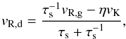 (C.1)where vR,g is the gas radial velocity, η is the ratio of the gas pressure gradient to the stellar gravity in the radial direction, and we consider vR,g = 0 since we are at equilibrium. Figure C.2 shows the evolution of the particle radial velocity in the first ten orbits for the implicit (red) and semi-implicit (grey) integrators together with the analytic solution (black) obtained from Eq. (C.1). The particle drift speed reaches almost immediately the expected drift speed. The semi-implicit integrator reaches the equilibrium speed on a longer timescale than the fully implicit one only for the lower stopping time (smaller particles).
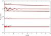 |
Fig. C.2 Evolution of the particle drift speed in the first ten orbits for particles with different stopping times. The analytic solution obtained from Eq. (C.1) is plotted with a black line, while the drift speed obtained from the semi-implicit and fully implicit integrators are displayed with red and grey lines, respectively. |
All Tables
All Figures
|
Fig. 1 Stopping time at the beginning of the simulation for the different particle sizes modelled. |
| In the text | |
|
Fig. 2 Radial drift velocity profile at the equilibrium for the different particle sizes modelled. |
| In the text | |
|
Fig. 3 Gas surface density (top panel) and vorticity profile (bottom panel) after 100 orbits. |
| In the text | |
|
Fig. 4 Gas surface density (top panel) and vorticity distribution (bottom panel) at the end of the simulation for the massive cores case. |
| In the text | |
|
Fig. 5 Distribution of cm-sized particles at different time steps (50, 60, 70, 80 orbital times) at the ring’s inner edge for the massive cores case. The evolution of two vortices in a frame co-moving with the disk at 1.3 au is shown. The vortex centre orbits the central star with a velocity close to the background Keplerian speed, which promotes particle trapping inside the vortex. |
| In the text | |
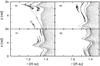 |
Fig. 6 Same as Fig. 5 but for a single massive core at r = 1. |
| In the text | |
|
Fig. 7 Dust normalised surface density distribution for the m- (first panel), dm- (second panel), cm- (third panel), and mm-sized (fourth panel) particles disk and two equal-mass 10 Mth cores at r = 1,2 at four different times (50, 100, 300, 600 orbital times) for each case. |
| In the text | |
|
Fig. 8 Particle distribution near the inner massive planetary core location for mm- (top left), cm- (top right), dm- (bottom left), and m-sized (bottom right) particles at the end of the simulation. The velocity vectors of the particles with respect to the planet are shown and the colour scale highlights the radial velocity component. |
| In the text | |
|
Fig. 9 Distribution of dm-sized particles at the end of the simulation of the two massive cores. The particle ring between the two planets shrinks with time until it clumps in a few stable points that form a pentagon-like structure with an orbit close to the 5:3 MMR with the inner planet at r = 1.4. |
| In the text | |
|
Fig. 10 Gas surface density (top panel) and vorticity distribution (bottom panel) at the end of the intermediate mass cores simulation. |
| In the text | |
|
Fig. 11 Dust normalised surface density distribution for the m- (first panel), dm- (second panel), cm- (third panel), and mm-sized (fourth panel) particles disk and two equal-mass 5 Mth cores at r = 1,2 at four different times (50, 100, 300, 600 orbital times) for each case. |
| In the text | |
|
Fig. 12 Particle distribution near the inner intermediate mass planetary core location for mm- (top left), cm- (top right), dm- (bottom left) and m-sized (bottom right) particles at the end of the simulation. The velocity vectors of the particles with respect to the planet are shown and the colour scale shows the relative radial velocity. |
| In the text | |
|
Fig. 13 Gas surface density (top panel) and vorticity distribution (bottom panel) at the end of the simulation for the two low mass cores. |
| In the text | |
|
Fig. 14 Dust normalised surface density distribution for the m- (first panel), dm- (second panel), cm- (third panel), and mm-sized (fourth panel) particles disk and two equal-mass 1 Mth cores at r = 1,2 at four different times (50, 100, 300, 600 orbital times) for each case. |
| In the text | |
|
Fig. 15 Particle surface density (top panel) and eccentricity profile (bottom panel) at the end of the simulation for the different particle species. |
| In the text | |
|
Fig. 16 Particle distribution near the inner low mass planetary core location for mm- (top left), cm- (top right), dm- (bottom left), and m-sized (bottom right) particles at the end of the simulation. The velocity vectors of the particles with respect to the planet are shown and the colour scale shows the relative radial velocity. |
| In the text | |
|
Fig. 17 Mass transfer through the planet position of mm-sized particles for the 1 thermal mass planet, which is unable to effectively filtrate them. The particles are plotted together with their velocity vectors and the colour scale indicates their radial velocities. |
| In the text | |
|
Fig. 18 Top panel: deprojected image from the mm continuum of HL Tau. Bottom panel: cross-cuts at PA = 138° through the peak of the mm continuum of HL Tau ALMA Partnership et al. (2015). |
| In the text | |
|
Fig. 19 Top panel: final mm-dust surface density distribution for an inner low mass core and an outer intermediate mass core. Bottom panel: relative surface density distribution. |
| In the text | |
|
Fig. 20 Top panel: dust distribution for the mm-sized particles disk and two planetary cores of ~10 and ~20 M⊕ after 250 orbits of the inner planet. Bottom panel: relative surface density distribution (red solid curve) where the distribution of the higher disk mass case (from Fig. 19 has been overplotted (blue dashed curve). |
| In the text | |
|
Fig. A.1 Disk surface density after 20 inner planetary orbits for the isothermal case (top panel) and fully radiative case (bottom panel) where the self-gravity of the disk is considered. |
| In the text | |
|
Fig. C.1 Orbital evolution of a dust particle released at r = 1, φ = 0, with vφ = 0.7 for the different integrators adopted in the simulations (red and green curves) compared to the solution from an explicit integrator (black curve). |
| In the text | |
|
Fig. C.2 Evolution of the particle drift speed in the first ten orbits for particles with different stopping times. The analytic solution obtained from Eq. (C.1) is plotted with a black line, while the drift speed obtained from the semi-implicit and fully implicit integrators are displayed with red and grey lines, respectively. |
| In the text | |
Current usage metrics show cumulative count of Article Views (full-text article views including HTML views, PDF and ePub downloads, according to the available data) and Abstracts Views on Vision4Press platform.
Data correspond to usage on the plateform after 2015. The current usage metrics is available 48-96 hours after online publication and is updated daily on week days.
Initial download of the metrics may take a while.