| Issue |
A&A
Volume 584, December 2015
|
|
|---|---|---|
| Article Number | A17 | |
| Number of page(s) | 9 | |
| Section | Stellar atmospheres | |
| DOI | https://doi.org/10.1051/0004-6361/201526647 | |
| Published online | 13 November 2015 | |
Modelling of variability of the chemically peculiar star ϕ Draconis⋆
1 Department of Theoretical Physics and Astrophysics, Masaryk University, Kotlářská 2, 611 37 Brno, Czech Republic
e-mail: prvak@physics.muni.cz
2 Institute of Astrophysics, University of Vienna, Türkenschanzstraße 17, 1180 Vienna, Austria
Received: 1 June 2015
Accepted: 7 September 2015
Context. The presence of heavier chemical elements in stellar atmospheres influences the spectral energy distribution of stars. An uneven surface distribution of these elements, together with flux redistribution and stellar rotation, are commonly believed to be the primary causes of the variability of chemically peculiar (CP) stars.
Aims. We aim to model the photometric variability of the CP star ϕ Dra based on the assumption of inhomogeneous surface distribution of heavier elements and compare it to the observed variability of the star. We also intend to identify the processes that contribute most significantly to its photometric variability.
Methods. We use a grid of TLUSTY model atmospheres and the SYNSPEC code to model the radiative flux emerging from the individual surface elements of ϕ Dra with different chemical compositions. We integrate the emerging flux over the visible surface of the star at different phases throughout the entire rotational period to synthesise theoretical light curves of the star in several spectral bands.
Results. The synthetic light curves in the visible and in the near-UV regions are in very good agreement with the observed variability of the star. The lack of usable far-UV measurements of the star precludes making any conclusions about the correctness of our model in this spectral region. We also obtained 194 new BVRI observations of ϕ Dra and improved its rotational period to P = 1 ḍ 716500(2).
Conclusions. We show that the inhomogeneous distribution of elements, flux redistribution, and rotation of the star are fully capable of explaining the stellar variability in the visible and the near-UV regions. The flux redistribution is mainly caused by bound-free transitions of silicon and bound-bound transitions of iron.
Key words: stars: chemically peculiar / stars: early-type / stars: variables: general / stars: individual: ϕ Dra
BVRI photometry of Phi Dra is only available at the CDS via anonymous ftp to cdsarc.u-strasbg.fr (130.79.128.5) or via http://cdsarc.u-strasbg.fr/viz-bin/qcat?J/A+A/584/A17
© ESO, 2015
1. Introduction
The star ϕ Dra (HD 170000 = HR 6920) is one of the brightest known CP stars. It was mentioned in the work of Maury & Pickering (1897), where it is classified as Group VII and marked peculiar. It is a multiple hierarchical system (e.g. Tokovinin 2008) containing visual (A, B) and spectroscopic (Aa, Ab) binary pairs.
It has been known for many years that the brightest component Aa is variable in some spectral regions (e.g. Kukarkin et al. 1969; Schöneich & Hildebrandt 1976). The observed variability is strongest in the far-ultraviolet (UV) region of the spectrum. In the near-UV and in the visible the variability is much weaker, and it is in antiphase to the far-UV variations of the star (Jamar 1977). This kind of variability has been observed in some other CP stars (e.g. α2 CVn), and it is typically explained by the inhomogeneous horizontal surface distribution of heavier elements, spectral energy redistribution, and rotation of the star (e.g. Molnar 1973).
Bound-bound transitions in the absorption lines of heavier elements, as well as bound-free transitions in the areas with increased metallicity cause absorption of a significant portion of the radiative energy in the far-UV part of the spectrum. This inevitably leads to an increase in the temperature in the stellar atmosphere (the backwarming effect), and the radiative flux in the near-UV and in the visible increases, so that the overall energy emitted by the star remains unchanged and the energy equilibrium is maintained. As the star rotates, we can observe variability in individual spectral regions as the areas with different chemical composition move across the visible stellar surface.
It is possible to derive surface abundance maps with observations of the line profile variations of various chemical elements throughout the entire rotational period of the star. To this end, techniques like Doppler imaging (DI) and magnetic Doppler imaging (MDI) are commonly used with success (e.g. Rice et al. 1989; Khokhlova et al. 2000; Piskunov & Kochukhov 2002; Kochukhov & Bagnulo 2004; Lüftinger et al. 2010a,b; Bohlender et al. 2010).
Availability of sufficiently detailed atomic data and high quality model atmospheres (e.g. Lanz & Hubeny 2007) allows us to accurately compute the emergent flux from stellar atmospheres with various chemical compositions. Putting these together with the abundance maps, it is possible to compute the emergent flux from individual regions of the atmospheres of the CP stars and, integrating the flux over the visible surface of the star repeatedly for different rotational phases, model the photometric variability in various spectral regions. This approach may serve as a test of the theory, our comprehension of the physical processes taking place in stellar atmospheres, the accuracy of atomic data and model atmospheres, and the correctness of the abundance maps.
This method has been used in the past to show that the photometric variations of several CP stars are caused by inhomogeneous distribution of various chemical elements. For example, the light variations of HD 37776 in the u, v, b, and y bands of the Strömgren photometric system are caused by spots of helium and silicon (Krtička et al. 2007). Similarly, Krtička et al. (2009) showed that most of the variability of HR 7224 can be explained by inhomogeneous distribution of silicon and iron. In the case of ε UMa, iron and chromium are responsible for the variability (Shulyak et al. 2010). Krtička et al. (2012) explained most of the variability of CU Vir by the inhomogeneous distribution of silicon and iron, but they were unable to fully explain the variations of the star in the region of 2000–2500 Å.
We intend to use the same technique to model the light variations of ϕ Dra using the abundance maps obtained from Kuschnig (1998a). Our preliminary results were published in Prvák et al. (2014).
2. Modelling of the SED variability
Our aim is to compare synthetic light curves, derived from our models based on maps constructed from the spectroscopy obtained at Observatoire de Haute-Provence using the Aurélie spectrograph Kuschnig (1998a; see also Kuschnig 1998b) to the ten-colour photometry by Musielok et al. (1980). Because of the large time gap between these two data sets, we had to improve the rotational period of the star and test its stability.
2.1. Our photometric observations
The studied star ϕ Dra with its V = 4.22 mag belongs to the brightest chemically peculiar stars in the northern hemisphere, which negatively influenced its photometric monitoring. Despite this, we have collected 673 individual photometric measurements covering forty years (1974–2013) – see Table 1 for the list of observations. The last item represents new measurements, which we obtained using a small refractor. The observations were performed at the Masaryk University Observatory (2 nights) and at the Brno Observatory and Planetarium (15 nights) from May to July 2013. Only the 12 best nights were used for the period analysis. Observing equipment consisted of a photographic lens Jupiter 3.5/135 mm (lens speed/focal length) and a Moravian Instruments CCD camera G2-0402 with Johnson-Cousins BVRI photometric filters. The angular resolution was only 14′′/pixel and thus it was not enough for angular separation of the fainter visual B component (actual distance around 0.5′′, see Fig. 9). The CCD images were calibrated in a standard way (dark frame and flat field corrections). The C-Munipack software1 (Motl 2009) which is based on DAOPHOT (Stetson 1987) was used for this processing and for differential ensemble photometry. Stars HD 169666 and HD 171044 were used as comparison stars.
2.2. Observed light variation: rotational period
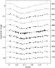 |
Fig. 1 Light curves of ϕ Dra in 11 photometric colours with effective wavelengths from 350 to 770 nm (on the right) plotted versus the new ephemeris with zero phase at the maximum (Eq. (3)). Grey full lines are the fits calculated by the simple model of ϕ Dra light variability (Eq. (1)). Light curves are vertically shifted to better display the light variability. Areas of individual symbols are proportional to the weight of the measurement. |
We modelled the observed photometric variations in the range from 350 to 770 nm by a simple phenomenological relation (see Fig. 1) assuming a linear ephemeris, 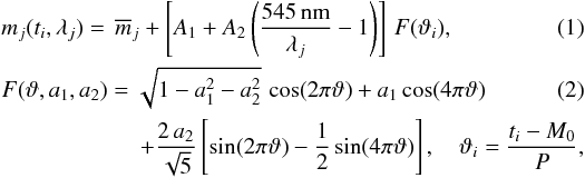 where mj(ϑi,λj) is a magnitude of the jth data subset obtained in the photometric filter with the effective wavelength λj in nm, ti is JDhel time of the ith measurement,
  is the mean magnitude of the jth data subset, A1 and A2 are amplitudes expressed in magnitudes, ϑ is a phase function, F(ϑ,a1,a2) is a normalised second order harmonic polynomial with a maximum at the phase ϕ = floor(ϑ) = 0, a1 and a2 are dimensionless parameters, M0 is the time of the basic extremum of the function F(ϑ), and P is the period.
The parameters were found by non-linear robust regression (a brief description is given in Mikulášek et al. 2003), which effectively eliminates outliers. After some iteration we found the following linear ephemeris,  (3)where E is an integer. The other model parameters are a1 = 0.214(3), a2 = −0.477(3), A1 = −0.0134(3) mag, and A2 = −0.0149(3) mag. The total amplitude at 345 nm is 0.047 mag; the amplitude at 770 nm is 0.020 mag.
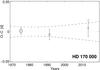 |
Fig. 2 O–C diagram for ϕ Dra calculated versus a new linear ephemeris (Eq. (3)). Areas of the circles are proportional to the weight of individual O–C values. The dashed lines denote 1-σ uncertainty of a light curve maximum time prediction. |
We recalculated the rotational phases of the abundance maps based on these new values. The improved ephemeris has resulted in a shift of the modelled light curves by about 0.16 in phase compared to the ephemeris used by Kuschnig (1998a). There are no signs of period variations (see Fig. 2).
2.3. Model atmospheres and synthetic spectra
For the modelling of the variability of ϕ Dra, we used the stellar parameters adopted from Kuschnig (1998a). A list of these parameters, including the ranges of abundances of the elements, for which the abundance maps were available, is given in Table 2. Here, the abundances are given as εel = log (Nel/Ntot).
Parameters of ϕ Dra from spectroscopy (Kuschnig 1998a).
We calculated a grid of model atmospheres for several different chemical compositions in order to cover the range of abundances across the surface of the star (the individual values of the abundances used are listed in Table 3). The atomic data were taken from Lanz & Hubeny (2007), and are based on Mendoza et al. (1995), Butler et al. (1993), Kurucz (1994, 2009), Nahar (1996, 1997), Bautista (1996), and Bautista & Pradhan (1997)2.
Given the very weak variability of helium and titanium abundances and their low values (see Table 2), we decided to exclude these two elements from the adopted abundance grid and use only a single value (the mean value) for each of them throughout the computations. This allowed us to significantly reduce the number of model atmospheres to be calculated.
Abundances used for model atmospheres.
The model atmospheres were computed using the TLUSTY code (Lanz & Hubeny 2007). They were all LTE plane-parallel models, because the NLTE effects do not have significant influence on the light variability of CP stars (Krtička et al. 2012). We also assumed the effective temperature Teff and the surface gravity log g to be constant across the entire stellar surface (see Table 2). We assumed a generic value of the microturbulent velocity vturb = 2.0 km s-1. The angle-dependent emergent specific intensities I(λ,θ,εSi,εCr,εFe) were computed using the SYNSPEC code.
2.4. Variability of the radiative flux
Parameters of the Gaussian functions used to approximate the transmissivity of the used filters of the ten-colour system.
The intensity Ic(θ,εSi,εCr,εFe) in the photometric colour c emerging from a stellar atmosphere with abundances εSi,εCr, and εFe can be determined by integrating the specific intensity over the wavelengths, 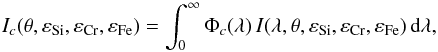 (4)where Φc(λ) is the response function for colour c. We modelled the variability in the coloursU, P, X, Y, Z, V, HR, and S of the ten-colour photometric system (see Schöneich & Hildebrandt 1976), which we approximated by Gauss functions. The parameters of these functions can be found in Table 4.
The entire surface of the star was subdivided into a grid of 68 × 33 elements, which corresponds to the resolution of the abundance maps. For each of these surface elements, the corresponding intensity was calculated based on the abundances taken from the abundance maps by means of a trilinear interpolation in the grid of synthetic spectra.
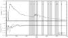 |
Fig. 3 Upper plot: emergent flux from a reference model atmosphere with εSi = −4.6, εCr = −6.7, and εFe = −5.1. Lower plot: emergent flux from the model atmospheres with modified abundance of individual elements minus the flux from the reference model. All fluxes were smoothed by a Gaussian filter with a dispersion of 10 Å to show the changes in continuum, which are important for SED variability. The passbands of the ten-colour photometric system are shown in the graph as grey areas. |
The total radiative flux fc in a colour c of a star with radius R∗ detected by an observer at the distance D at any given rotational phase can be found using the formula (Mihalas 1978)  (5)The magnitude difference in a colour c is then defined as
 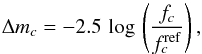 (6)where
  is the reference flux determined in such a way that, averaged over an entire rotational period, the resulting magnitude difference will be equal to zero.
3. Results
3.1. Influence of chemical elements
The chemical elements present in stellar atmospheres influence the way the energy is distributed in the spectrum. Bound-bound and bound-free transitions are responsible for the absorption of a significant portion of the energy in some parts of the spectrum. For the sake of the energetic balance in the stellar atmosphere, this energy has to be re-emitted in other regions of the spectrum. This is demonstrated in Fig. 3, where we show the spectral energy distribution (SED) emergent from a reference stellar atmosphere with low abundance of silicon, iron, and chromium and the differences in the energy distribution between the reference atmosphere and stellar atmospheres with an overabundance of silicon, iron, and chromium. Higher abundance of heavier elements leads to higher brightness in the visible region. This is shown in Fig. 4 where we plot the magnitude differences between the flux calculated with enhanced abundance of individual elements and the flux emergent from the reference atmosphere.
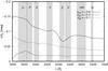 |
Fig. 4 Magnitude difference Δmλ between the emergent fluxes calculated with an enhanced abundance of the individual elements and the reference flux |

Silicon and iron cause strong absorption in the far-UV part of the spectrum, especially between 1100 and 1500 Å. The absorption in the iron lines is a characteristic feature for the adjacent UV region 1500–2000 Å. In addition, most of the energy absorbed by silicon in the far-UV region 1100–1500 Å is re-emitted in the region with wavelengths 1500–2000 Å. The visible part of the spectrum is mostly dominated by re-emission of the energy absorbed by iron with some contribution of silicon. A high concentration of iron absorption lines suppresses the contribution of iron to the light variability in a small region around 5200 Å. This leads to a typical flux depression (Kupka et al. 2004).
Some influence of chromium is also visible in Figs. 3 and 4, but it is weaker than the influence of silicon and iron as a result of a relatively low maximum chromium abundance. Consequently, chromium does not have a significant impact on the general character of the variability of the star.
3.2. Variability of the star
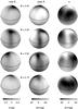 |
Fig. 5 Emergent intensity from the surface of ϕ Dra at various rotational phases at wavelengths of 1400 Å (left panel), 2500 Å (middle panel), and in the U-band of the ten-colour system (right panel). The intensities are displayed as −2.5log (I/I0), where I0 is a reference intensity chosen in such a way that the resulting logarithm, averaged over the entire stellar surface, is equal to zero. |
We model the variability of ϕ Dra using abundance maps adopted from Kuschnig (1998a). Both silicon and iron maps feature a large area with a higher abundance than the rest of the surface. Figure 5 shows the emergent intensity from the various points across the stellar disk at various rotational phases in several spectral regions. Areas with high silicon and iron abundance appear as dark spots on the stellar surface in the far-UV, whereas they appear bright in the visible as a result of the flux redistribution. The opposite holds for regions with lower silicon and iron abundance.
The light curves of the star are shown in Fig. 6. The modelled curves are compared to the photometric observations (Musielok et al. 1980). Both the amplitude and the shape of the modelled curves agree with the observations. The variability of the star is most pronounced in the U-band, while in the Z-band the amplitude is the smallest of all modelled curves. The shape of the curves remains roughly the same in all passbands in the visible spectrum and bears a strong resemblance to a sine function. The light curve in the Z-band, both the modelled and the observed, is slightly shifted in phase compared to the other curves.
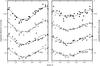 |
Fig. 6 Light curves of ϕ Dra in the passbandsU, P, X, Y, Z, V, HR, and S of the ten-colour photometric system. Modelled curves (solid lines) are compared to observational data (Musielok et al. 1980). The light curves have been vertically shifted to better demonstrate the light variability. |
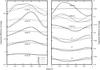 |
Fig. 7 Light curves of ϕ Dra synthesised using the abundance maps of the individual elements separately, compared to the overall variability of the star (solid line) in several Gaussian passbands with the dispersion of 20 Å in the UV and the passbands U,Z, and S of the ten-colour photometric system. The light curves have been shifted vertically to better demonstrate the variability. We note the very different vertical scales of the two panels. |
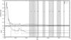 |
Fig. 8 Upper plot: predicted amplitude (half of the difference between the maximum and the minimum magnitude of the star) of the photometric variability of the star in Gaussian passbands with a dispersion of 20 Å as a function of wavelength. Lower plot: phase of the minimum of the variability of the star in the same passbands plotted against the wavelength. |
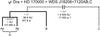 |
Fig. 9 Diagram of the multiple system ϕ Dra with expected values for angular and absolute distances between components (total semi-major axes between binary pairs) and their orbital periods (Liška, in prep.). |
3.3. Effect of the individual elements
In order to see how the individual chemical elements affect the variability of the star, we synthesised the light curves of the star using only one of the abundance maps at a time, keeping the abundances of the other elements constant. These light curves are shown in Fig. 7 in selected UV and visual passbands.
The variability is strongest in the region around 1200 Å, mostly due to the absorption by silicon. The modelled light curve at 1400 Å qualitatively resembles the observed light curve presented by Jamar (1977), the observed light curve having somewhat larger amplitude (approx. 0.15 mag compared to the 0.096 mag amplitude for the modelled one). However, since the original data from the paper are not available and important information is missing, such as the ephemeris or the width of the passband used, we cannot sensibly plot the observed light curve together with the modelled one. At about 1570 Å, we can observe the transition between the inversely correlated absorption and re-emission regions for silicon. The contribution of silicon to the overall variability of the star at this wavelength is practically null and the light variations are caused almost exclusively by iron absorption. An analogous situation, where the iron light curve shows practically no variations, can be seen at approximately 1940 Å. Chromium does not contribute significantly to the light curves at any wavelength as a result of its relatively low abundance.
The light curves showing the variability due to the individual elements vary in amplitude and sign, but they retain their shape and phase throughout the examined spectrum. The curves are, however, shifted in phase relative to each other, because the individual elements are distributed differently across the stellar surface.
On the other hand, the shape of the light curves obtained using all abundance maps changes significantly with the wavelength. The shape of the resulting light curve depends on the ratio of the amplitudes of the components of the variability due to the individual chemical elements and their orientation, i.e. whether the particular element contributes to the variability by absorption or by re-emission due to the backwarming effect.
While there are some zero-amplitude regions in the UV and the visible, separating the absorbing and the re-emitting parts of the spectrum for the individual elements, there is no such region for the resulting variability of the star. The reason is that the zero-amplitude regions for the various examined elements are located at different wavelengths. This demonstrates that the concept of the null wavelength region, i.e. where no variability shows at a given wavelength, is an oversimplification that may occur only as a result of observations that are not precise enough.
Figure 8 shows the predicted amplitude of the light variations in the narrow-band passbands across the UV and the visible spectrum. The amplitude is greatest in the region 1200–1400 Å, dropping quickly with increasing wavelength. In the lower plot of Fig. 8, we show the phase position of the light minimum of the variations at various wavelengths plotted together with the minima of the variability due to silicon and iron. The position of the minima of the variability caused by individual elements practically do not change, except for a few sudden changes, which actually represent the transitions between the absorbing and the re-emitting regions for silicon and iron, where the curves flip vertically, so that the minima become maxima and vice versa. The phase of the light minimum of the resulting light curve drifts fluidly between the minima of the individual elements, gravitating toward the one with the greater amplitude.
4. Influence of stellar multiplicity
The studied object (Aa) is a part of a multiple stellar system (Beardsley 1969; Andrade 2005, Liška, in prep.). It is the brighter component of an SB1-type spectroscopic binary (Aa, Ab) with a more distant, visual companion (B). There is a possible fourth (optical) component C presented in the Washington Double Star Catalogue (Mason et al. 2001). A diagram of the system is given in Fig. 9.
The multiplicity of the system may affect the light curve modelling. We therefore investigate the influence of the other components on our results.
4.1. Influence of light time effect
Each of the components influences the observed period of CP variability by the light time effect (LiTE), which could be visible in the O–C diagram. Semi-amplitude AAa of LiTE can be calculated directly from RV changes (Beardsley 1969). We obtained AAa ~ 0.0012 day ≐ 104 s with orbital period (127.990(4) days, Liška, in prep.) of system Aab. This is under the accuracy of available measurements. The B component causes higher LiTE amplitude AAab ~ 0.2 day (maximum value). This value is relatively high, but the whole cycle takes several hundred years (e.g. Andrade 2005 estimated an orbital period of 307.8 yr). Consequently, our analysed observations in a 40-yr interval were influenced only slightly, so the rotational period can be accurately approximated by a constant value  (see Fig. 2).
4.2. Influence of RV changes
Kuschnig (1998a) used spectra for DI obtained during 5 days in term JDhel 2 449 797.404–2 449 802.684 that correspond to the orbital phases 0.05–0.09 of the inner system Aab determined with elements adopted from Liška (in prep.). The semi-amplitude of the radial velocity of the inner orbit of the Aa component was found to be KAa = 29.0(1.3) km s-1. Therefore, the radial velocity of the Aa component would have changed during Kuschnig’s observations by almost 11 km s-1; for a wavelength of 5000 Å, this would roughly correspond to a shift of Δλ5000 = 0.18 Å. This is low in comparison to the rotational velocity of the star (95 km s-1, see Table 2). Changes in RV due to the visual B component in this short term interval is also negligible due to the long period and low semi-amplitude KAab ~ 5 km s-1 (maximum value).
4.3. Contribution of the components to the flux
The B star is fainter than Aab in the Hipparcos band by about ΔHp = 1.445(10) mag (ESA 1997), in the Tycho bands ΔBT = 1.50(1) mag, ΔVT = 1.42(1) mag (Fabricius & Makarov 2000), and in red and infrared ΔR = 1.42(2) mag, ΔI = 1.33(3) mag (Rutkowski & Waniak 2005). Flux ratios FAab/FB in these bands are 0.264 (Hp), 0.251 (BT), 0.270 (VT), 0.270 (R), 0.294 (I). From these values, it is evident that 21–23% of the total flux in optical bands belongs to the B component. The observed amplitude of brightness variations for the Aab component is about 21–23% higher after subtracting the B component flux. We do not have enough information about the Ab component, but we assume its contribution to the total flux is negligible. The influence of the B component on the photometric variability is not negligible, but it is probably partially compensated by its influence on the line strengths and derived abundances. The influence of the B component may be one of the reasons why the observed amplitude of the flux variations at 1400 Å is slightly larger than the predicted amplitude.
5. Discussion
There are several simplifications that can affect our results. In our computations, we neglected the effects of the magnetic field of the star. ϕ Draconis has a moderate magnetic field with a poloidal component Bp ≈ 3 kG (Landstreet & Borra 1977). However, as demonstrated by Khan & Shulyak (2006), magnetic fields of this magnitude do not have significant impact on the SED variability of CP stars.
The abundance maps were derived using a mean stellar atmosphere, as opposed to computing local model atmospheres for the individual elemental abundances present on the stellar surface. This means the influence of the modified, varying chemical composition on the internal structure of the atmosphere was not taken into account during the mapping. According to some studies (e.g. Stift et al. 2012), this introduces an error in the computations, which may result in incorrect abundance maps. However, the good agreement between our models and the observations indicates that the accuracy of the abundance maps is sufficient. The detailed tests of Doppler mapping techniques also support this conclusion (Kochukhov et al. 2012).
6. Conclusions
Using our own data, as well as the archive photometric data, we have found a new linear ephemeris for the light maximum based on Eq. (3)in the optical region of stellar spectra. There are no signs of period inconstancy of the star.
We successfully modelled the SED variations of the star ϕ Dra in the UV and the visible regions. The assumption of an inhomogeneous horizontal surface distribution of heavier elements, together with spectral energy redistribution and the rotation of the star, can fully explain the observed light variations.
The variability of the star is caused mainly by bound-bound transitions of iron and bound-free transitions of silicon. While the influence of silicon is more significant in the near and far UV spectrum, the visible region is mostly dominated by re-emission due to the presence of iron. Chromium also contributes to the light variations, but its role in the variability of the star is much less significant than that of iron and silicon.
The variability of the star is caused by multiple chemical elements, with different horizontal distributions, which has several consequences. The general shape of the light curve strongly depends on the wavelength. The light curves in the various spectral regions are shifted in phase with respect to each other. There is no zero-amplitude region in the UV or in the visible, separating the absorbing and the re-emitting parts of the spectrum with inversely correlated variability.
Our models nicely predict the variability of the star in the visible, including both the shape and the amplitude of the light variations. However, our results may be slightly influenced by the multiplicity of the system. The models also predict the slight shift in phase for the light curve in the Z-band of the ten-colour system, which agrees with observations. The lack of quantitative UV observations of the star makes it is impossible for us to verify the correctness of our models in this part of the spectrum. This is very unfortunate because the processes that are most interesting for the variability of the star occur in this particular region.
This work indicates that the variability of most CP stars is caused by inhomogeneous surface distribution of heavier elements and rotation of the star. It is a strong argument in favour of the correctness and accuracy of the abundance maps, the atomic data, and the model atmospheres.
Acknowledgments
The authors of this paper acknowledge the support of the grants GA ČR P209/12/0217, MŠMT 7AMB14AT015 (WTZ CZ 09/2014), and in final phases of GA ČR 13-10589S. This work was supported by the Brno Observatory and Planetarium. T.L. acknowledges support by the Austrian FFG within ASAP11 and by the FWF NFN projects S11601-N16 and S116 604-N16.
References
- Andrade, M. 2005, IAUDS, 157, 1 [NASA ADS] [Google Scholar]
- Bautista, M. A. 1996, A&AS, 119, 105 [NASA ADS] [CrossRef] [EDP Sciences] [Google Scholar]
- Bautista, M. A., & Pradhan, A. K. 1997, A&AS, 126, 365 [NASA ADS] [CrossRef] [EDP Sciences] [Google Scholar]
- Beardsley, W. R. 1969, Publications of the Allegheny Observatory of the University of Pittsburgh, 8, 91 [NASA ADS] [Google Scholar]
- Bohlender, D. A., Rice, J. B., & Hechler, P. 2010, A&A, 520, A44 [NASA ADS] [CrossRef] [EDP Sciences] [Google Scholar]
- Butler, K., Mendoza, C., & Zeippen, C. J. 1993, J. Phys. B, 26, 4409 [NASA ADS] [CrossRef] [Google Scholar]
- ESA 1997, The Hipparcos and Tycho Catalogs, SP, 1200 [Google Scholar]
- Fabricius, C., & Makarov, V. V. 2000, A&A, 356, 141 [NASA ADS] [Google Scholar]
- Jamar, C. 1977, A&A, 56, 413 [NASA ADS] [Google Scholar]
- Khan, S. A., & Shulyak, D. 2006, A&A, 448, 1153 [NASA ADS] [CrossRef] [EDP Sciences] [Google Scholar]
- Khokhlova, V. L., Vasilchenko, D. V., Stepanov, V. V., & Romanyuk, I. I. 2000, Astron. Lett., 26, 177 [Google Scholar]
- Kochukhov, O., & Bagnulo, S. 2004, A&A, 414, 613 [NASA ADS] [CrossRef] [EDP Sciences] [Google Scholar]
- Kochukhov, O., Wade, G. A., & Shulyak, D. 2012, MNRAS, 421, 3004 [NASA ADS] [CrossRef] [Google Scholar]
- Kukarkin, B. V., Kholopov, P. N., Efremov, Y. N., et al. 1969, General Catalogue of Variable Stars, Volume_1 (Moskva: Astronomical Council of the Academy of Sciences in the USSR) [Google Scholar]
- Krtička, J., Mikulášek, Z., Zverko, J., & Žižňovský, J. 2007, A&A, 470, 1089 [NASA ADS] [CrossRef] [EDP Sciences] [Google Scholar]
- Krtička, J., Mikulášek, Z., Henry, G. W., et al. 2009, A&A, 499, 567 [NASA ADS] [CrossRef] [EDP Sciences] [Google Scholar]
- Krtička, J., Mikulášek, Z., Lüftinger, T., et al. 2012, A&A, 537, A14 [NASA ADS] [CrossRef] [EDP Sciences] [Google Scholar]
- Kupka, F., Paunzen, E., Iliev, I. Kh., & Maitzen, H. M. 2004, MNRAS, 352, 863 [NASA ADS] [CrossRef] [Google Scholar]
- Kurucz, R. L. 1994, Kurucz CD-ROM 22, Atomic Data for Fe and Ni (Cambridge: SAO) [Google Scholar]
- Kuschnig R., 1998a, Ph.D. Thesis, Univ. of Vienna [Google Scholar]
- Kuschnig, R. 1998b, Contributions of the Astronomical Observatory Skalnate Pleso, 27, 418 [NASA ADS] [Google Scholar]
- Landstreet, J. D., & Borra, E. F. 1977, ApJ, 212, L43 [NASA ADS] [CrossRef] [Google Scholar]
- Lanz, T., & Hubeny, I. 2007, ApJS, 169, 83 [CrossRef] [Google Scholar]
- Lüftinger, T., Kochukhov, O., Ryabchikova, T., et al. 2010a, A&A, 509, A71 [NASA ADS] [CrossRef] [EDP Sciences] [Google Scholar]
- Lüftinger, T., Fröhlich, H.-E., Weiss, W. W., et al. 2010b, A&A, 509, A43 [NASA ADS] [CrossRef] [EDP Sciences] [Google Scholar]
- Mason, B. D., Wycoff, G. L., Hartkopf, W. I., Douglass, G. G., & Worley, C. E. 2001, AJ, 122, 3466 [Google Scholar]
- Maury, A. C., & Pickering, E. C. 1897, Annals of Harvard College Observatory, 28, 1 [Google Scholar]
- Mendoza, C., Eissner, W., Le Dourneuf, M., & Zeippen, C. J. 1995, J. Phys. B, 28, 3485 [NASA ADS] [CrossRef] [Google Scholar]
- Mihalas, D. 1978, Stellar Atmospheres (San Francisco: Freeman & Co.) [Google Scholar]
- Mikulášek, Z., Žižňovský, J., Zverko, J., et al. 2003, Contr. Obs. Skalnaté Pleso, 33, 29 [Google Scholar]
- Molnar, M. R. 1973, ApJ, 179, 527 [NASA ADS] [CrossRef] [Google Scholar]
- Musielok, B., Lange, D., Schoenich, W., et al. 1980, Astron. Nachr., 301, 71 [Google Scholar]
- Nahar, S. N. 1996, Phys. Rev. A, 53, 1545 [NASA ADS] [CrossRef] [PubMed] [Google Scholar]
- Nahar, S. N. 1997, Phys. Rev. A, 55, 1980 [NASA ADS] [CrossRef] [Google Scholar]
- Piskunov, N., & Kochukhov, O. 2002, A&A, 381, 736 [NASA ADS] [CrossRef] [EDP Sciences] [Google Scholar]
- Prvák, M., Krtička, J., Mikulášek, Z., Lüftinger, T., & Liška, J. 2014, Putting A Stars into Context: Evolution, Environment, and Related Stars, 214 [Google Scholar]
- Rice, J. B., Wehlau, W. H., & Khokhlova, V. L. 1989, A&A, 208, 179 [NASA ADS] [Google Scholar]
- Rutkowski, A., & Waniak, W. 2005, PASP, 117, 1362 [NASA ADS] [CrossRef] [Google Scholar]
- Schöneich, W., Hildebrandt, G. 1976, Astron. Nachr., 297, 39 [NASA ADS] [CrossRef] [Google Scholar]
- Shulyak, D., Krtička, J., Mikulášek, Z., et al. 2010, A&A, 524, A66 [CrossRef] [EDP Sciences] [Google Scholar]
- Stetson, P. B. 1987, PASP, 99, 191 [NASA ADS] [CrossRef] [Google Scholar]
- Stift, M. J., Leone, F., & Cowley, C. R. 2012, MNRAS, 419, 2912 [NASA ADS] [CrossRef] [Google Scholar]
- Tokovinin, A. 2008, MNRAS, 389, 925 [NASA ADS] [CrossRef] [Google Scholar]
All Tables
Parameters of the Gaussian functions used to approximate the transmissivity of the used filters of the ten-colour system.
All Figures
|
Fig. 1 Light curves of ϕ Dra in 11 photometric colours with effective wavelengths from 350 to 770 nm (on the right) plotted versus the new ephemeris with zero phase at the maximum (Eq. (3)). Grey full lines are the fits calculated by the simple model of ϕ Dra light variability (Eq. (1)). Light curves are vertically shifted to better display the light variability. Areas of individual symbols are proportional to the weight of the measurement. |
| In the text | |
|
Fig. 2 O–C diagram for ϕ Dra calculated versus a new linear ephemeris (Eq. (3)). Areas of the circles are proportional to the weight of individual O–C values. The dashed lines denote 1-σ uncertainty of a light curve maximum time prediction. |
| In the text | |
|
Fig. 3 Upper plot: emergent flux from a reference model atmosphere with εSi = −4.6, εCr = −6.7, and εFe = −5.1. Lower plot: emergent flux from the model atmospheres with modified abundance of individual elements minus the flux from the reference model. All fluxes were smoothed by a Gaussian filter with a dispersion of 10 Å to show the changes in continuum, which are important for SED variability. The passbands of the ten-colour photometric system are shown in the graph as grey areas. |
| In the text | |
|
Fig. 4 Magnitude difference Δmλ between the emergent fluxes calculated with an enhanced abundance of the individual elements and the reference flux |
| In the text | |
|
Fig. 5 Emergent intensity from the surface of ϕ Dra at various rotational phases at wavelengths of 1400 Å (left panel), 2500 Å (middle panel), and in the U-band of the ten-colour system (right panel). The intensities are displayed as −2.5log (I/I0), where I0 is a reference intensity chosen in such a way that the resulting logarithm, averaged over the entire stellar surface, is equal to zero. |
| In the text | |
|
Fig. 6 Light curves of ϕ Dra in the passbandsU, P, X, Y, Z, V, HR, and S of the ten-colour photometric system. Modelled curves (solid lines) are compared to observational data (Musielok et al. 1980). The light curves have been vertically shifted to better demonstrate the light variability. |
| In the text | |
|
Fig. 7 Light curves of ϕ Dra synthesised using the abundance maps of the individual elements separately, compared to the overall variability of the star (solid line) in several Gaussian passbands with the dispersion of 20 Å in the UV and the passbands U,Z, and S of the ten-colour photometric system. The light curves have been shifted vertically to better demonstrate the variability. We note the very different vertical scales of the two panels. |
| In the text | |
|
Fig. 8 Upper plot: predicted amplitude (half of the difference between the maximum and the minimum magnitude of the star) of the photometric variability of the star in Gaussian passbands with a dispersion of 20 Å as a function of wavelength. Lower plot: phase of the minimum of the variability of the star in the same passbands plotted against the wavelength. |
| In the text | |
|
Fig. 9 Diagram of the multiple system ϕ Dra with expected values for angular and absolute distances between components (total semi-major axes between binary pairs) and their orbital periods (Liška, in prep.). |
| In the text | |
Current usage metrics show cumulative count of Article Views (full-text article views including HTML views, PDF and ePub downloads, according to the available data) and Abstracts Views on Vision4Press platform.
Data correspond to usage on the plateform after 2015. The current usage metrics is available 48-96 hours after online publication and is updated daily on week days.
Initial download of the metrics may take a while.