| Issue |
A&A
Volume 584, December 2015
|
|
|---|---|---|
| Article Number | A60 | |
| Number of page(s) | 10 | |
| Section | Planets and planetary systems | |
| DOI | https://doi.org/10.1051/0004-6361/201526082 | |
| Published online | 20 November 2015 | |
Dissipation in rocky planets for strong tidal forcing
Institute of Geophysics, University of Göttingen,
Friedrich-Hund-Platz 1,
37077, Göttingen, Germany
e-mail: niels.clausen@geo.physik.uni-goettingen.de; andreas.tilgner@geo.physik.uni-goettingen.de
Received: 12 March 2015
Accepted: 4 September 2015
Aims. We plan to reproduce a previously published calculation for the tidal dissipation in Io and extend the employed model to investigate the heat transport mechanism in Io and the thickness of Io’s asthenosphere. Additionally, we apply this model to an exoplanet and obtain insights into the dependencies of the modified tidal quality factor (Q′) on the size of the planet and its orbital eccentricity.
Methods. Tidal dissipation depends on the heat transport mechanism. For strong tidal forcing an equilibrium between heat transport by convection and heat production by tidal dissipation can be obtained that determines the tidal dissipation. By this means, we checked whether convection is the dominant heat transport mechanism in Io. The tidal dissipation also depends on the interior model of Io. We considered various asthenosphere thicknesses and determined which of these gives results compatible with observations. We determined the modified tidal quality factors (Q′) for Corot 7 b for various orbital parameters, but in a way that tidal forcing is strong. We used convection and melt migration as possible heat transport mechanism. We repeated this for a hypothetical planet with the size and density of Io on the orbit of Corot 7 b.
Results. We find that a heat transport dominated by convection in Io is possible, but the grain sizes need to be smaller than 2.2 mm. For larger grain sizes melt migration is the dominant heat transport mechanism. Moreover, Io’s asthenosphere needs to be thicker than 100 km. The computation of the modified tidal quality factors (Q′) for Corot 7 b and a planet with the size and density of Io on the orbit of Corot 7 b show that Q′ is scattered over several orders of magnitude, but a value of 100 for Q′ is an acceptable estimate for a rocky planet under strong tidal forcing.
Key words: convection / planets and satellites: general / planets and satellites: dynamical evolution and stability / planets and satellites: individual: Io / planets and satellites: terrestrial planets / planet-star interactions
© ESO, 2015
1. Introduction
It is important to know the energy dissipated by tides to determine the long-term orbital evolution of planetary systems. The tidal dissipation is usually parameterized by the tidal quality factor Q or the modified tidal quality factor Q′ (see Sect. 2.2). Earth has Q ≈ 12 (Murray & Dermott 1999), which is on the same order as the quality factor of other terrestrial planets in our solar system. According to Goldreich & Soter (1966), these lie in the range 10 ≤ Q ≤ 190.
Often, Q′ = 100 is assumed for terrestrial exoplanets because this is approximately the modified tidal quality factor of Earth (Murray & Dermott 1999). However, Efroimsky (2012) claimed that it is inappropriate to approximate tidal quality factors of super-Earths by that of Earth because the higher self-gravitation in a super-Earth compared to an Earth-mass object leads to less efficient tidal damping in super-Earths. Hansen & Murray (2015) suggested that a Q′ of approximately 10 is a reasonable a priori estimate for terrestrial planets. They obtained the best match with the observed eccentricity distribution of terrestrial exoplanets with this value, assuming a scenario for planet formation (that fixes the initial conditions for the orbital evolution) as in Hansen & Murray (2013).
Estimates of Q′ remain controversial. Q′ depends not only on the size of the object, but also on the orbital frequency (Efroimsky & Lainey 2007). Henning & Hurford (2014) recently investigated the dependence of Q′ on the orbital period and on the interior structure of the planet. They considered multilayer planets with the possibility of oceans and ice regions.
While the principles underlying the theoretical calculation of tidal dissipation are relatively clear for a rocky body such as Io, there is some confusion in the literature about certain details of the computation, and most importantly about the numerical values obtained for Io as a standard application. Since the study of exoplanetary systems and their orbital history revives interest in computations of tidal dissipation, we take the opportunity to revisit the classical calculation outlined in Moore (2003). In this model, the tidal forcing is strong enough to start thermal convection and to establish a stationary state in which the tidally dissipated heat is transported by convection to the planet’s surface. The temperature profile established within the planet determines its viscosity and hence the tidal dissipation in a self-consistent fashion. We apply this model to Io, also for comparison with previous work, and then to the exoplanet Corot 7b to probe the sensitivity of Q′ on orbital parameters, planet size, and asthenosphere thickness.
2. Theoretical background
2.1. Tidal dissipation
This section summarizes the methods used in previous studies to compute the tidal dissipation that we also used here. The dissipation DT due to the quasi-static deformation of a planet is given by (e.g., Segatz et al. 1988)  (1)with Ωp the orbital angular velocity, e the eccentricity of the orbit, G the gravitational constant, and Rp planet radius. For our purpose, Eq. (1) is accurate enough, but for high eccentricities the equation underestimates tidal heating (Leconte et al. 2010). The factor ℑ(k2) is the imaginary part of the tidal Love number and has to be determined from a model of the interior structure of the planet. If the shear modulus is different from zero, the deformation of the planet is determined by the solution of the six coupled ordinary differential equations (ODEs; Eq. (1.51) of Sabadini & Vermeersen 2004). The treatment of a liquid core is the same as in Saito (1974). From the solution of these ODEs, ℑ(k2) can be determined. These equations require the density ρ, μ, and η to be given as a function of radius and are solved in the frequency domain. Assuming that the Maxwell model describes the viscoelastic response of the material well, the equation contains the variable
  given by
  (2)where the orbital frequency Ωp is the frequency at which the planet is forced, and μ and η depend on temperature and possibly pressure, as determined by a rheological law, to be specified below. The density ρ is assumed to be constant in single layers, and the gravitational acceleration g is obtained accordingly from Poisson’s equation. The system is forced by the tidal potential
 ![\begin{eqnarray} &&\Phi=r^2\Omega_\mathrm{p}^2e\Bigg(-\frac{3}{2}P^0_2(\cos\vartheta)\cos(\Omega_\mathrm{p} t) \nonumber\\ &&\hspace*{5mm}+ \frac{1}{4} P_2^2( \cos\vartheta)\left[3\cos\Omega_\mathrm{p} t\cos2\varphi+4\sin\Omega_\mathrm{p} t\sin 2 \varphi\right]\Bigg), \end{eqnarray}](/articles/aa/full_html/2015/12/aa26082-15/aa26082-15-eq22.png) (3)where r is the radius from the center of mass of the planet, ϑ and ϕ are the colatitude and longitude with zero longitude at the near pole, t is the time, and
(3)where r is the radius from the center of mass of the planet, ϑ and ϕ are the colatitude and longitude with zero longitude at the near pole, t is the time, and  and
and  are associated Legendre functions.
The system of ODEs mentioned above is linear, and the response involves only spherical harmonics of degree 2. We solved these equations, complemented with the boundary conditions (Eq. (1.127) of Sabadini & Vermeersen 2004), with a shooting method (as opposed to Sabadini & Vermeersen 2004, who treated the same system with a propagator matrix method).
The rheological law specifying μ and η used for this study is similar to the one used in Moore (2003). The temperature dependence of μ and η is given by  B is a dimensionless melt fraction coefficient. We used B = 25 and B = 40. We chose B = 25 because Mei et al. (2002) reported this value for diffusion creep (see also Karato 2013), and B = 40 because it is the highest value that Moore (2003) used. As in Moore (2003), we assumed the solidus temperature Tsol to be at 1598 K and the critical temperature Tcrit at 1600 K. φ is the volume melt percentage. It increases linearly from the solidus to the liquidus at a rate of 1% per Kelvin. The liquidus is assumed to be at 1698 K. The shear modulus is zero above the disaggregation temperature Tdis. Disaggregation occurs at ~30% partial melting (Moore 2001; Scott & Kohlstedt 2006). The figures in this study are partly plotted up to 1670 K, which corresponds to a melt fraction of 72%. We recall that the solid matrix may already have disaggregated at ~1630 K.
Viscosity and shear modulus as a function of temperature are plotted in Fig. 1.
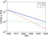 |
Fig. 1 Viscosity and shear modulus as a function of temperature. |
This rheological law, plugged into the set of ODEs (Eq. (1.51) of Sabadini & Vermeersen 2004), allows computing ℑ(k2) and the tidal dissipation in Eq. (1) as a function of temperature. Functions DT(T) appear in subsequent figures. We used the equations for the layered planet in configurations in which only one temperature is relevant: the model planet consists of four layers at most. With increasing distance from center to the surface, there may be a liquid core that does not participate in the tidal dissipation because of its low viscosity, a “deep mantle” with fixed values for μ and η, an “asthenosphere” that obeys the rheological law above, and finally a “lithosphere” with fixed values for μ and η. For the M1 model (Table 4) the contribution to the tidal dissipation of deep mantle and lithosphere is small because of their high viscosities (Segatz et al. 1988). The temperature of the asthenosphere is assumed uniform across this layer, and the tidal dissipation DT(T) must be computed as a function of the asthenosphere temperature T. The density in the deep mantle, asthenosphere, and lithosphere is approximated by a single-density ρm, but these layers have different μ and η.
Notation and parameters that are treated as constants.
This one adjustable temperature is fixed by the condition that the tidally dissipated heat is transported across the planet and radiated from the surface into space. The laws determining the heat flux in a planet are a matter of ongoing research. Here, we present a few relations that have been used in the past in similar studies of tidal dissipation.
According to a numerical calculation of time-dependent stagnant lid convection in a spherical shell with internal heating and free slip boundary conditions (Reese et al. 2005)  (6)with the Nusselt number
  (7)the Rayleigh number
  (8)and the Frank-Kamenetskii parameter
  (9)For a strictly temperature-dependent viscosity,
  (Reese et al. 1999; Moore 2003). F is the heat flux, dc is the thickness of the convecting layer without the stagnant lid (in the four-layer model, dc equals the thickness of the asthenosphere), Ti the interior temperature and Ts the surface temperature. For stagnant lid convection Ti = Tl + arhγ-1, with Tl the temperature at the bottom of the lid, and arhγ-1 the temperature jump across the rheological boundary layer where arh is a numerical coefficient. We used arh = 3.2 for time-dependent stagnant lid convection, following Reese et al. (2005). For the remaining constants see Table 1. With Eq. (9)for θ, Eq. (6)can be written as
  (10)which is analogous to Eq. (13) of Reese et al. (2005). The last equation shows that convection beneath the stagnant lid is similar to isoviscous convection with an effective driving temperature γ-1.
For steady-state stagnant lid convection in a spherical shell with internal heating and free slip boundary conditions (Reese et al. 1999)  (11)and arh = 3.7.
For plate tectonic convection with internal heating, we used a scaling as in O’Connell & Hager (1980) (12)with a flow geometry constant a2 ~ 1 and the critical Rayleigh number Rac ~ 1100 and
  (13)Because RaF/ Rai = Nu, Eq. (12) is equivalent to
 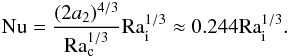 (14)The correctness of this scaling is supported by newer numerical simulations by Wolstencroft et al. (2009), who found scaling relations that differ only slightly.
It is assumed that the scaling relations for Nu(Ra) used here with a Rayleigh number exponent of 1/3 are also applicable for convection in a material with a high melt fraction and high Rayleigh number because this scaling is in accordance with boundary layer theory (Turcotte & Schubert 2002; Douce 2011), and numerical simulations at high Rayleigh number generally differ only little from this scaling, see the review by Ahlers et al. (2009) and references therein.
In summary, the convective heat flux is given by a relation of the form 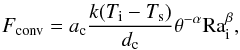 (15)where ac, α, and β are constants depending on the the Nu(Rai) relation of choice. This flux must equal the tidal heat flux through the surface
 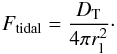 (16)For the four-layer model of Io and Corot 7 b we calculated with a fixed rl = Rp − dlit, with dlit the lithosphere thickness (see Table 4). For plate tectonic convection we approximated rl by Rp. For these cases, equating Eqs. (15) and (16) fixes Ti if Ts is given so that DT is computable. For stagnant lid convection in the homogeneous mantle model (this is a two-layer model with a liquid core and a solid mantle), we calculated rl by taking into account the thermal effect of the lithosphere, as was done by Moore (2003). In this model, the upper surface of the convection zone is the bottom of the lid, which is located at radius rl and has a temperature Tl, so that conditions need to be found to determine rl, Tl, and Ti. These are the balance between tidal and convective heat fluxes and two expressions for Tl (Reese et al. 1999)
 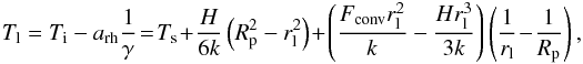 (17)with
  (18)being the rate of internal heat generation (in W/m3).
In the study of Io below, Ts is assumed given by observations. In exoplanet studies, Ts is determined from the tidal dissipation and the irradiance of the host star (Henning et al. 2009)  (19)σsb is the Stefan-Boltzmann constant, ϵr the emissivity, A the albedo, Lstar the stellar luminosity, and a the semi-major axis. Finally, the temperature T in DT(T) is identified with Ti.
2.2. Tidal quality factor
We calculated the tidal quality factor according to Murray & Dermott (1999) (20)with E0 the peak energy stored during the cycle
  (21)With Eq. (1) this gives
  (22)The modified tidal quality factor is
  (23)The modified tidal quality factor is defined such that it only depends on ℑ(k2), which is the quantity that appears in Eq. (1), and that for a homogeneous liquid sphere (k2 = 3/2) Q′ = Q.
2.3. Melt migration
In a partially molten mantle, magma transport can be important for the heat transport, as is the case, for example, in Io’s asthenosphere (Moore 2001). The governing equations for heat transport by melt through the mantle are as follows (Moore 2001).
-
The conservation of mass
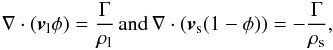 (24)with vl and vs the velocities of the liquid and solid components, ρl and ρs the liquid and solid densities, φ the melt volume fraction, and Γ the melt production rate (in kg m-3 s-1). In contrast to Moore (2001), we took the difference in the densities of liquid and solid in Eq. (24) into account.
 -
The Darcy flow equation
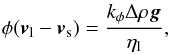 (25)with the permeability kφ = b2φn/τ, b is a typical grain size, τ is a constant that depends on the exponent n, ηl is the viscosity of the liquid, and Δρ the density contrast between liquid and solid material. In our calculations we chose n = 2.6 and τ = 60 (Miller et al. 2014). These expressions are valid as long as the solid matrix does not disaggregate and the melt does form an interconnected network.
 -
The conservation of energy
 (26)with L the latent heat of fusion.
The system of Eqs. (24)–(26)can be written as two first-order equations for φ and vl by eliminating Γ and vs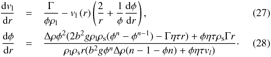 From Eq. (24) we can deduce
 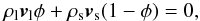 (29)this equation is valid globally. If only parts of the melting zone are considered, the flux of mass into or out of the zone needs to be included, for instance, due to an upwelling mantle. Equations (25), (26), and (29) can be rearranged such that the heat flux due to melt migration FM is given by
  (30)For | g | we used the surface gravity. Δρ = ρs − ρl and ηl were calculated with the MELTS program (Ghiorso & Sack 1995), and for ρs we used the mantle density ρm. The radial component of the liquid and solid velocities is approximated through the absolute value of vl and vs, respectively. Equation (30)is only correct if the melting zone has a constant melt volume fraction. This would roughly be the case for large enough grain sizes. We checked the validity of this approach by solving the six coupled ODEs (Eq. (1.51) of Sabadini & Vermeersen 2004) with a fixed viscosity and shear modulus in the deep mantle and the lithosphere, but in the asthenosphere the viscosity was determined by additionally solving Eqs. (27)and (28)with initial conditions φ = 0.01 and vl = 0 at the base of the molten zone. With the obtained value for φ and the resulting temperature, the viscosity can be determined self-consistently and becomes thereby depth dependent in the asthenosphere. The heating rate per volume is given by Eq. (39) in Beuthe (2013).
3. Validation
The code computing ℑ(k2) through a solution of coupled ODEs (Eq. (1.51) of Sabadini & Vermeersen 2004) was validated by a comparison with various other studies, in particular with Segatz et al. (1988) and Sotin et al. (2009). As Beuthe (2013) noted, Segatz et al. (1988) omitted a factor 2π in the angular frequency. The factor 2π in the angular frequency is also missing in other publications (Fischer & Spohn 1990; Moore & Schubert 2000; Moore 2003), as the validation of our code has shown. Thus all viscosity values in Segatz et al. (1988) need to be divided by 2π. The viscosity values here are adjusted through a division by 2π for this validation. After this correction, the results obtained with our code agree well with results reported by Segatz et al. (1988) and Sotin et al. (2009).
4. Results
4.1. Tidal dissipation of Io
The estimation of the tidal dissipation in Io by Moore (2003) led to a heat flux of ≈2 × 10¹³ W. This is lower than the observed surface flux of 0.6−1.6 × 10¹⁴ W (Moore et al. 2007). Moore (2003) therefore concluded that either Io is currently out of thermal equilibrium or another heat transport mechanism such as melt migration determines Io’s thermal state. Lainey et al. (2009) showed that Io is close to thermal equilibrium, so that only another heat transport mechanism is left as an explanation. As mentioned in Sect. 3, Moore (2003) calculated with an incorrect viscosity because a factor 2π was missing. Figure 2a is calculated as in Moore (2003) with the incorrect viscosity and (b) is calculated with the correct viscosity, but for both figures a Nu(Ra) scaling according to Eq. (11)was used. Figure 2 shows that the final dissipation values do not change much because of the incorrect viscosity.
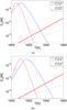 |
Fig. 2 Tidal dissipation (DT) and transported heat assuming steady-state convection (ssC) for two different rheologies and incorrect viscosity a) and correct viscosity b) for the homogeneous mantle model. The model parameter are listed in Tables 1–3. Nu(Ra) is given according to Eq. (11). |
Notation and parameters for Io.
Parameter values for the rheology model according to Fischer & Spohn (1990).
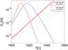 |
Fig. 3 Tidal dissipation (DT) and transported heat assuming time-dependent convection (tdC) for two different rheologies for the homogeneous mantle model. The model parameters are listed in Tables 1–3. Nu(Ra) is given according to Eq. (6). |
Moore (2003) stated that he used β = 1/3, α = 4/3, and ac = 1.3–2.5 in the relation between Nu and Rai, but we were unable to reproduce his results (for instance, his Fig. 4) with this β, α, and ac. Instead, the results in Moore (2003) were presumably obtained with the heat transfer law for steady-state convection, Eq. (11), or very similar parameters. Figure 3 shows the results for time-dependent convection, Eq. (6). This changes the results from Moore (2003) noticeably. Most importantly, one finds a dissipation rate of DT ≈ 1.1 × 10¹⁴ W, compatible with the observed value, without invoking melt migration. However, at the interior temperature of the equilibrium found in Fig. 3, the rheological law assumes a nonzero melt fraction, so that some contribution of melt migration to the total heat transport is likely. This motivated us to study more detailed models, in which Io consists of a liquid core, a deep mantle with zero melt fraction, an asthenosphere, and a lithosphere. We defined the asthenosphere as the zone with a nonzero melt fraction. The results for different asthenosphere thicknesses are shown in Fig. 4. The behavior of the tidal dissipation as a function of the asthenosphere temperature DT(T) depends sensitively on the asthenosphere thickness, while the convective heat flux according to Eqs. (6) and (7) does not.
In the following, we assumed 1014 W as the nominal value of Io’s tidal dissipation and a Nu(Ra) scaling according to Eq. (6). At the temperature at which the tidal dissipation equals 1014 W, the convective heat flux must be less than or equal to 1014 W. This requires an asthenosphere thickness of at least 100 km, as seen in Fig. 4. If it is less than 1014 W, a contribution by melt migration is possible. Melt migration as the dominant mechanism (i.e., transporting more heat than convection) requires an asthenosphere thickness larger than 200 km. Figure 4 only shows results for B = 25 and not B = 40 because the difference between the convection-dissipation equilibrium values for different B values is negligible, at least for 25 ≤ B ≤ 40, as is made plausible in Figs. 2 and 3 and as was reported by Moore (2003). An asthenosphere with a rock melt fraction of 20% or more and at least 50 km thickness was recently inferred from magnetic data by Khurana et al. (2011). An asthenosphere thinner than 100 km is similarly unlikely because it requires a presumably too high disaggregation temperature to obtain a tidal dissipation of 1014 W. Figure 4 also includes for comparison a convective heat transport for a Nu(Ra) scaling according to Eq. (6), but with −1.3 and 0.3 as exponents instead of −4/3 and 1/3. With this scaling, melt migration is the dominant heat transport for an asthenosphere thicker than 100 km.
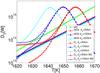 |
Fig. 4 Tidal dissipation (DT) and transported heat assuming time-dependent convection (tdC and tdCb) for three different asthenosphere thicknesses. The model parameters are listed in Tables 1–4; if not otherwise stated, the values for model 1, M1, were used. Nu(Ra) is given according to Eq. (6) (tdC) and according to Eq. (6), but with exponents −1.3 and 0.3 instead of −4/3 and 1/3 (tdCb). B = 25. |
For simplicity, the melt fraction was assumed to be constant throughout the asthenosphere. Especially if heat transport by melt migration is important, a viscosity change with depth similar as in Fig. 1 of Moore (2001) is expected. The lowest viscosity is found at the top of the melting zone; we call this viscosity in the following ηBL. The tidal dissipation with a depth-dependent viscosity due to melt migration is smaller than the tidal dissipation with a constant viscosity ηc for ηc = ηBL and identical asthenosphere thickness as long as ηBL is lower than the viscosity at which the tidal dissipation peaks because then the tidal dissipation decreases if the viscosity increases. We confirmed these relationships and inequalities by simulations. The convective heat flux is only little affected by a depth-dependent viscosity if the Rayleigh number is defined by the viscosity ηBL, at least for high Nusselt numbers and a strong viscosity contrast due to the temperature dependence of the viscosity (Dumoulin et al. 1999). Therefore the obtained asthenosphere thicknesses in this section can be viewed as lower bounds because we need thicker asthenospheres for a depth dependent viscosity due to melt migration to obtain the same tidal dissipation as in the constant viscosity case. Below we show that our determined asthenosphere thicknesses are not only a lower bound, they are even a proper estimate for the thickness with depth-dependent viscosity.
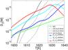 |
Fig. 5 Heat transported by melt migration (mm) for three different grain sizes, assuming time-dependent convection (tdC) and tidal heat (DT) for three different asthenosphere thicknesses, model M1. See Tables 1–4 for the model parameters. Nu(Ra) is given according to Eq. (6) for time-dependent convection and according to Eq. (30)for melt migration. B = 25. |
Now we include melt migration. Moore (2001) calculated according to his Eqs. (6) and (7) that all of Io’s tidal heat can be transported by melt migration for melt fractions below 20%, depending on the exact parameters. But both crystal size and melt viscosity are uncertain. Carr et al. (1998) assumed a crystal size ~1 mm, and Keszthelyi et al. (2004) suggested that the liquid viscosity ηl varies between 1 and 400 Pa s and the density contrast between 520 and 690 kg/m3 as partial melting varies between 50% and 20%. Here we calculated with a viscosity ηl and a density contrast Δρ obtained with the MELTS program (Ghiorso & Sack 1995), as in Keszthelyi et al. (2004) for the LL-chrondite model (Keszthelyi et al. 2004). In Figs. 5 and 6 the heat flux for melt migration was calculated according to Eq. (30).
With a significant contribution by melt migration to the heat flux, the obtained tidal heat depends on the melt fraction coefficient B because in the Darcy law the viscosity of the liquid is used and the tidal dissipation depends on the viscosity of the partially molten rock.
If our parameterizations are correct and we have a 400 km thick asthenosphere, for instance, with B = 25 and grain size b = 5 mm, the obtained tidal dissipation is 9.1 × 10¹³ W, see Fig. 5. The contribution by convection can be ignored in this case.
These calculations show that taking into account melt migration, stable equilibra are also possible where the slope of the tidal heating curve DT(T) is positive, see Figs. 5 and 6, for example. For a heat transport by convection alone, this is generally not the case because an equilibrium between heat transport and tidal heat flux is stable only if the slope of the tidal heating curve is smaller than the slope of the heat transport curve, otherwise a runaway temperature increase would occur.
From Figs. 5 and 6 we can deduce that it is possible only for small grain sizes that convection is the dominant heat transport mechanism, smaller than 2.2 mm for B = 40 and even smaller for B = 25. If the tidal dissipation is 1014 W and convection dominates the heat transport, more than 5 × 10¹³ W must be carried by convection. The curves for heat fluxes due to convection and melt migration intersect at 5 × 10¹³ W for a grain size of 2.2 mm in Fig. 6. The tidal dissipation of 1014 W is realized for an asthenosphere thickness slightly thicker 200 km for this grain size and the temperature of the intersection point. We can deduce from this figure that a a tidal dissipation of 1014 W for B = 40 is mainly transported by convection for smaller grain sizes than 2.2 mm and by melt migration for larger sizes. For B = 25 the analogous grain size boundary lies at lower values, see Fig. 5.
In the remainder of this section we assume that disaggregation occurs at a viscosity of 1012 Pa s, which is already a low viscosity for a partial molten mantle with a competent solid matrix (Kohlstedt & Mackwell 2009). This means we assume Tdis as the temperature corresponding to a viscosity of 1012 Pa s. Only if a mushy magma ocean, a mix of crystals and melt, were to exist would lower viscosities than 1012 Pa s be possible. The existence of such a mushy zone is questionable, however, because of the separation process. Stevenson (2002) predicted that a mushy magma ocean thicker than 20 km would be unstable over geologic timescales. For viscosities smaller than 1012 Pa s, equilibria between heat transport and tidal heat production would be possible where the slope of the DT(T) curve is negative. But to obtain a tidal dissipation of 1014 W at a higher temperature than the peak temperature, the grain size needs to be smaller than 0.5 mm (see Figs. 5 and 6) and the asthenosphere needs to be thick, for b = 0.5 mm thicker than 600 km.
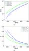 |
Fig. 7 Grain size ba) and corresponding melt fraction at the top of the melting zone b) for which a tidal dissipation of 1014 W is obtained as a function of asthenosphere thickness, calculated with a constant melt fraction in the asthenosphere (φ const.) according to Eq. (30)and a variable (φ vari) as described in Sect. 2.3. The convective heat transport is neglected. |
From Fig. 7a we can deduce that our calculations with a constant melt fraction in the asthenosphere are roughly correct. For this plot we considered melt migration as the sole heat transport mechanism. The largest discrepancy is present for an asthenosphere thickness of 250 km and B = 25, the obtained grain size differs in this case by a factor of 2. The grain size is only poorly known to begin with, therefore this difference is acceptable. Figure 7b also confirms that our estimated asthenosphere sizes deduced from Fig. 4 are appropriate for a rough estimate and are a lower bound. Comparing the models with variable and constant viscosity, we find that for a tidal dissipation of 1014 W and any given asthenosphere thickness, the melt fraction is slightly higher at the top of the molten zone for the case of a variable viscosity profile. The difference is strongest for B = 40 and a 250 km thick asthenosphere. For this case the melt fraction differs by 10%, which corresponds to a temperature difference of 10 K. The Nu(Ra) relation is not exactly known, so that a temperature difference of 10 K is of little importance. Furthermore, because the melt fractions on top are always higher for the variable viscosity profile, our asthenosphere thicknesses are a lower bound.
It can be deduced from Fig. 8 that with increasing asthenosphere thickness, melt migration becomes more important and the grain size needs to be larger to obtain a tidal dissipation of 1014 W. If viscosities lower than 1012 Pa s were attainable, a dominant contribution by convection would also be possible for large asthenosphere thicknesses. Viscosities as low as this are not considered in Fig. 8, but our calculations revealed that it is possible to obtain a tidal dissipation in the range of the observed one for a viscosity lower than 1012 Pa s, an asthenosphere thicker than 785 km, and a grain size smaller than 100 μm. For asthenosphere thicknesses in the range from 200 km to 785 km, melt migration is always the dominant mechanism.
Parameters for the asthenosphere model of Io.
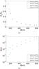 |
Fig. 8 Amount of heat transported by time-dependent convection (Dc) divided by the total heat transported by convection plus melt migration (DT) as a function of asthenosphere thickness a). The corresponding grain size b) was chosen such that the value of tidal dissipation is 1014 W, or 6 × 10¹³ W for small asthenosphere thicknesses, were a value of 1014 W was not accessible. Model M1 was used. For the model parameters see Tables 1–4. Nu(Ra) is given according to Eq. (6) for time-dependent convection and according to Eq. (30)for melt migration. |
4.2. Tidal dissipation of Corot 7 b
The tidal evolution of Corot 7b was computed among others by Rodríguez et al. (2011). It was commonly assumed by these authors that Q′ = 100 on the grounds that Corot 7b is a terrestrial planet (see also, e.g., Léger et al. 2011). We show in this section that reasonable assumptions about terrestrial exoplanets lead to values of Q′ scattered over several orders of magnitude, but Q′ = 100 is a realistic approximation.
In the following, we obtain Q′ for objects surrounding the host star of Corot 7b, which have either the size and density of Corot 7b, or the size and density of Io, and which have orbital periods P of either P = 2 d or P = 6 d.
We considered various heat transport mechanisms with the same rheology as for Io in the previous section, model M1, but for the deep mantle we used a higher viscosity, see Table 5.
For melt migration, the grain size b equals either 1 mm or 5 mm. The viscosity ηl and the density contrast Δρ were again calculated with the MELTS program (Ghiorso & Sack 1995) as in Keszthelyi et al. (2004) for the LL-chrondite model (see Keszthelyi et al. 2004). The surface temperature was determined with Eq. (19). Tdis was again assumed to be the temperature corresponding to a viscosity value of 1012 Pa s.
The results are summarized in Figs. 9–11, in which Q′ is given as a function of eccentricity e in a range of eccentricities that may plausibly be encountered during orbital evolution. For too high eccentricities, the tidal forcing is so strong that melt fraction coefficients higher than the melt fraction at the assumed disaggregation point would be necessary to transport the heat. This applies to the heat transport mechanism, convection, and melt migration. With increasing eccentricities the tidal dissipation curve is shifted to higher values for temperatures lower than Tdis. If the eccentricity exceeds a certain value, an intersection with the heat transport curve becomes impossible for a given Tdis. Therefore no Q′ values were obtained at high eccentricities. With a heat transport by convection and low eccentricities, it is possible that the tidal dissipation is too weak at any given temperature to maintain a heat flux compatible with the convective heat transport at that temperature, so that there can be no equilibrium between convective and tidal heat fluxes. For this case no Q′ can be determined, either.
From Figs. 9–11 it can be deduced that a Q′ of 100 is a realistic approximation for rocky planets under strong tidal forcing. The values for Q′ mainly lie between 10 and 1000. With melt migration as the dominant heat transport mechanism, Q′ higher than 1000 is only possible for thin asthenospheres at short periods or very high eccentricities.
The figures show that there is an influence of heat transport mechanism, eccentricity, orbital period, asthenosphere thickness, and size of the object on Q′. The asthenosphere thickness has a huge effect on Q′. Because asthenosphere thicknesses are currently not known for any exoplanet, it is not useful to describe the dependencies of Q′ on the other parameters in detail.
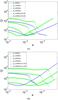 |
Fig. 9 Q′ as a function of eccentricity calculated with depth-dependent viscosity as described in Sect. 2.3 for a planet with the size and density of Corot 7 b and four different asthenosphere thicknesses. The contribution by a convective heat transport is not included in the calculation of Q′. Two different orbital periods a)P = 2 d and b) P = 6 d were considered. If not otherwise stated, b = 5 mm and B = 40. The model parameters are listed in Tables 1 and 3–5. |
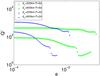 |
Fig. 10 As in Fig 9, but for a planet with the size and density of Io. The respective orbital period is quoted in the legend. See Tables 1–4 for the model parameters. |
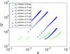 |
Fig. 11 Q′ as a function of eccentricity for stagnant lid convection (sl) and plate tectonic convection (pt) for a planet with the size and density of Corot 7 b and two different asthenosphere thicknesses. The contribution by melt migration is not included in the calculation of Q′. The respective orbital period is quoted in the legend. Nu(Ra) according to Eq. (6) (sl) and Eq. (14) (pt). The model parameters are listed in Tables 1 and 3–5. B = 25. |
Notation and parameters for Corot 7 b.
5. Conclusion and discussion
We investigated the tidal dissipation of rocky planets for planets with a near equilibrium tide, excluding dynamic tides such as the oceanic tides on Earth. Throughout this paper, “planet” denoted the tidally deformed body, whether a planet or a moon. Tidal forcing was assumed to be strong in the sense that there is a stable equilibrium between tidal dissipation and heat transport due to convection or melt migration. This equilibrium determines the tidal dissipation of the planet.
The method we used was adapted from Moore (2003; see also Fischer & Spohn 1990). This method is only applicable to planets whose heat budget is dominated by tides and solar or stellar radiation. Radiogenic and accretional heat production were ignored. Both the tidal dissipation rate and the convective heat flow depend on the viscosity, which in turn depends on temperature. Therefore the temperature had to be adjusted such that there was an equilibrium between tidal heat flow and convective heat flow. The heat flow due to melt migration in contrast depends on the viscosity of the liquid in the partially molten region, not on the viscosity of the partially molten rock. For melt migration, the equilibrium heat production therefore depends on the melt fraction coefficient and also on the grain size. It is more precise to take into account the depth dependence of the viscosity than using a single viscosity for the partial molten region. For a heat transport dominated by melt migration, this is possible by coupling Eq. (1.51) of Sabadini & Vermeersen (2004) with Eqs. (27)and (28).
Tidal dissipation was calculated for a body consisting of a solid mantle with a lithosphere, a convecting asthenosphere, and a liquid core. Stagnant lid, plate tectonic convection, and melt migration were considered.
We showed that the tidal dissipation of Io can be explained by an equilibrium between convection and tidal heat production. But for the basic assumptions, which entail that the Nu(Ra) scales according to Eq. (6) and that the lowest attainable viscosity is 1012 Pa s, a heat transport dominated by convection is only possible for an asthenosphere thinner than ~200 km, but thicker than ~100 km and grain sizes smaller than 2.2 mm if B ≤ 40. With an exponent of −1.3 and 0.3 instead of −4/3 and 1/3 in the Nu(Ra) relationship Eq. (6), as used in Fig. 4, a heat transport dominated by convection becomes more unlikely because then the asthenosphere needs to be thinner than ~100 km for a heat transport dominated by convection. But an asthenosphere thinner than ~100 km is unlikely because it requires a presumably too high disaggregation temperature to obtain a tidal dissipation of 1014 W.
Corot 7b was also investigated as an example of an exoplanet. The modified tidal quality factor Q′ of a planet depends on its size. This dependence was mentioned in Efroimsky (2012) as a result of a gravitational effect, whereas we also considered thermal effects here. The radius of exoplanets is usually well constrained by observations, while the eccentricity of their orbit is not. However, Q′ also depends on eccentricity and orbital frequency, as shown above, which also implies that Q′ varies during orbital history.
Another large uncertainty is introduced by the parameters characterizing the heat transport. These uncertainties add up to a range of plausible values for Q′ spanning several orders of magnitude. But our results suggest that a Q′ value of 100 is a realistic approximation for strong tidal forcing. The values for Q′ mainly lie in the range 10 to 1000, see Figs. 9–11.
Acknowledgments
The authors acknowledge research funding by Deutsche Forschungsgemeinschaft (DFG) under grant SFB 963/1, project A5.
References
- Ahlers, G., Grossmann, S., & Lohse, D. 2009, Rev. Mod. Phys., 81, 503 [NASA ADS] [CrossRef] [Google Scholar]
- Beuthe, M. 2013, Icarus, 223, 308 [NASA ADS] [CrossRef] [Google Scholar]
- Carr, M. H., Belton, M. J. S., Chapman, C. R., Davies, M. E., et al. 1998, Nature, 391, 363 [NASA ADS] [CrossRef] [Google Scholar]
- Douce, A. P. 2011, Thermodynamics of the Earth and Planets (Cambridge: Cambridge University Press) [Google Scholar]
- Dumoulin, C., Doin, M.-P., & Fleitout, L. 1999, J. Geophys. Res., 104, 12759 [NASA ADS] [CrossRef] [Google Scholar]
- Efroimsky, M. 2012, ApJ, 746, 150 [NASA ADS] [CrossRef] [Google Scholar]
- Efroimsky, M., & Lainey, V. 2007, J. Geophys. Res. Planets, 112, E12003 [NASA ADS] [CrossRef] [Google Scholar]
- Fischer, H.-J., & Spohn, T. 1990, Icarus, 83, 39 [NASA ADS] [CrossRef] [Google Scholar]
- Ghiorso, M. S., & Sack, R. O. 1995, Contrib. Mineral. Petrol., 119, 197 [NASA ADS] [CrossRef] [Google Scholar]
- Goldreich, P., & Soter, S. 1966, Icarus, 5, 375 [NASA ADS] [CrossRef] [Google Scholar]
- Hansen, B. M. S., & Murray, N. 2013, ApJ, 775, 1 [Google Scholar]
- Hansen, B. M. S., & Murray, N. 2015, MNRAS, 448, 1044 [NASA ADS] [CrossRef] [Google Scholar]
- Henning, W. G., & Hurford, T. 2014, ApJ, 789, 30 [NASA ADS] [CrossRef] [Google Scholar]
- Henning, W. G., O’Connell, R. J., & Sasselov, D. D. 2009, ApJ, 707, 1000 [NASA ADS] [CrossRef] [Google Scholar]
- Jacobson, R. A. 2003, JUP230 – JPL satellite ephemeris [Google Scholar]
- Karato, S. 2013, Physics and Chemistry of the Deep Earth (Wiley-Blackwell) [Google Scholar]
- Keszthelyi, L., Jaeger, W. L., Turtle, E. P., Milazzo, M., & Radebaugh, J. 2004, Icarus, 169, 271 [NASA ADS] [CrossRef] [Google Scholar]
- Khurana, K. K., Jia, X., Kivelson, M. G., et al. 2011, Science, 332, 1186 [NASA ADS] [CrossRef] [Google Scholar]
- Kohlstedt, D. L., & Mackwell, S. J. 2009, in Planetary Tectonics, eds. T. R. Watters, & R. A. Schultz (Cambridge University Press), 397 [Google Scholar]
- Lainey, V., Arlot, J.-E., & Karatekin, O., & Van Hoolst, T. 2009, Nature, 459, 957 [NASA ADS] [CrossRef] [PubMed] [Google Scholar]
- Leconte, J., Chabrier, G., Baraffe, I., & Levrard, B. 2010, A&A, 516, A64 [NASA ADS] [CrossRef] [EDP Sciences] [Google Scholar]
- Léger, A., Grasset, O., Fegley, B., et al. 2011, Icarus, 213, 1 [NASA ADS] [CrossRef] [Google Scholar]
- Mei, S., Bai, W., Hiraga, T., & Kohlstedt, D. L. 2002, Earth Planet. Sci. Lett., 201, 491 [NASA ADS] [CrossRef] [Google Scholar]
- Miller, K. J., Zhu, W., Montési, L. G. J., & Gaetani, G. A. 2014, Earth Planet. Sci. Lett., 388, 273 [NASA ADS] [CrossRef] [Google Scholar]
- Moore, W. B. 2001, Icarus, 154, 548 [NASA ADS] [CrossRef] [Google Scholar]
- Moore, W. B. 2003, J. Geophys. Res., 108, E8 [Google Scholar]
- Moore, W. B., & Schubert, G. 2000, Icarus, 147, 317 [NASA ADS] [CrossRef] [Google Scholar]
- Moore, B., Schubert, G., Anderson, J. D., & Spencer, J. R. 2007, in Io after Galileo: A new view of Jupiter’s volcanic moon, eds. R. M. C. Lopez, & J. R. Spencer (Springer), 89 [Google Scholar]
- Murray, C., & Dermott, S. 1999, Solar System Dynamics (Cambridge University Press) [Google Scholar]
- O’Connell, R., & Hager, B. 1980, in Physics of the Earth’s Interior, eds. A. Dziewonski, & E. Boschi (Amsterdam: North Holland Publ. Co.), 270 [Google Scholar]
- Rathbun, J. A., Spencer, J. R., Tamppari, L. K., et al. 2004, Icarus, 169, 127 [NASA ADS] [CrossRef] [Google Scholar]
- Reese, C. C., Solomatov, V. S., Baumgardner, J. R., & Yang, W.-S. 1999, Phys. Earth Planet. Inter., 116, 1 [NASA ADS] [CrossRef] [Google Scholar]
- Reese, C. C., Solomatov, V. S., & Baumgardner, J. R. 2005, Phys. Earth Planet. Inter., 149, 361 [NASA ADS] [CrossRef] [Google Scholar]
- Rodríguez, A., Ferraz-Mello, S., Michtchenko, T. A., Beaugé, C., & Miloni, O. 2011, MNRAS, 415, 2349 [NASA ADS] [CrossRef] [Google Scholar]
- Sabadini, R., & Vermeersen, B. 2004, Global Dynamics of the Earth (Dordrecht: Kluwer) [Google Scholar]
- Saito, M. 1974, J. Phys. Earth, 22, 123 [CrossRef] [Google Scholar]
- Schubert, G., Anderson, J., Spohn, T., & McKinnon, W. 2004, in Jupiter: The Planet, Satellites and Magnetosphere, eds. T. Bagenal, F. Dowling, & W. McKinnon (Cambridge University Press), 281 [Google Scholar]
- Scott, T., & Kohlstedt, D. 2006, Earth Planet. Sci. Lett., 246, 177 [NASA ADS] [CrossRef] [Google Scholar]
- Segatz, M., Spohn, T., Ross, M., & Schubert, G. 1988, Icarus, 75, 187 [NASA ADS] [CrossRef] [Google Scholar]
- Sotin, C., Tobie, G., Wahr, J., & McKinnon, W. B. 2009, in Europa, eds. R. Pappalardo, W. McKinnon, & K. Khurana (University of Arizona Space Science Series), 11, 85 [Google Scholar]
- Stevenson, D. J. 2002, in Eos. Trans. AGU 83. P12C-10 [Google Scholar]
- Tackley, P., Ammann, M., Brodholt, J., Dobson, D., & Valencia, D. 2013, Icarus, 225, 50 [NASA ADS] [CrossRef] [Google Scholar]
- Turcotte, D., & Schubert, G. 2002, Geodynamics (Cambridge: Cambridge University Press) [Google Scholar]
- Turtle, E. P., Jaeger, W. L., & Schenk, P. M. 2007, in Io after Galileo: A new view of Jupiter’s volcanic moon, eds. R. M. C. Lopez, & J. R. Spencer (Springer), 109 [Google Scholar]
- Wagner, F. W., Tosi, N., Sohl, F., Rauer, H., & Spohn, T. 2012, A&A, 541,A103 [NASA ADS] [CrossRef] [EDP Sciences] [Google Scholar]
- Wolstencroft, M., Davies, J., & Davies, D. 2009, Phys. Earth Planet. Inter., 176, 132 [Google Scholar]
All Tables
All Figures
|
Fig. 1 Viscosity and shear modulus as a function of temperature. |
| In the text | |
|
Fig. 2 Tidal dissipation (DT) and transported heat assuming steady-state convection (ssC) for two different rheologies and incorrect viscosity a) and correct viscosity b) for the homogeneous mantle model. The model parameter are listed in Tables 1–3. Nu(Ra) is given according to Eq. (11). |
| In the text | |
|
Fig. 3 Tidal dissipation (DT) and transported heat assuming time-dependent convection (tdC) for two different rheologies for the homogeneous mantle model. The model parameters are listed in Tables 1–3. Nu(Ra) is given according to Eq. (6). |
| In the text | |
|
Fig. 4 Tidal dissipation (DT) and transported heat assuming time-dependent convection (tdC and tdCb) for three different asthenosphere thicknesses. The model parameters are listed in Tables 1–4; if not otherwise stated, the values for model 1, M1, were used. Nu(Ra) is given according to Eq. (6) (tdC) and according to Eq. (6), but with exponents −1.3 and 0.3 instead of −4/3 and 1/3 (tdCb). B = 25. |
| In the text | |
|
Fig. 5 Heat transported by melt migration (mm) for three different grain sizes, assuming time-dependent convection (tdC) and tidal heat (DT) for three different asthenosphere thicknesses, model M1. See Tables 1–4 for the model parameters. Nu(Ra) is given according to Eq. (6) for time-dependent convection and according to Eq. (30)for melt migration. B = 25. |
| In the text | |
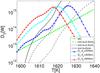 |
Fig. 6 As in Fig. 5, but for B = 40. |
| In the text | |
|
Fig. 7 Grain size ba) and corresponding melt fraction at the top of the melting zone b) for which a tidal dissipation of 1014 W is obtained as a function of asthenosphere thickness, calculated with a constant melt fraction in the asthenosphere (φ const.) according to Eq. (30)and a variable (φ vari) as described in Sect. 2.3. The convective heat transport is neglected. |
| In the text | |
|
Fig. 8 Amount of heat transported by time-dependent convection (Dc) divided by the total heat transported by convection plus melt migration (DT) as a function of asthenosphere thickness a). The corresponding grain size b) was chosen such that the value of tidal dissipation is 1014 W, or 6 × 10¹³ W for small asthenosphere thicknesses, were a value of 1014 W was not accessible. Model M1 was used. For the model parameters see Tables 1–4. Nu(Ra) is given according to Eq. (6) for time-dependent convection and according to Eq. (30)for melt migration. |
| In the text | |
|
Fig. 9 Q′ as a function of eccentricity calculated with depth-dependent viscosity as described in Sect. 2.3 for a planet with the size and density of Corot 7 b and four different asthenosphere thicknesses. The contribution by a convective heat transport is not included in the calculation of Q′. Two different orbital periods a)P = 2 d and b) P = 6 d were considered. If not otherwise stated, b = 5 mm and B = 40. The model parameters are listed in Tables 1 and 3–5. |
| In the text | |
|
Fig. 10 As in Fig 9, but for a planet with the size and density of Io. The respective orbital period is quoted in the legend. See Tables 1–4 for the model parameters. |
| In the text | |
|
Fig. 11 Q′ as a function of eccentricity for stagnant lid convection (sl) and plate tectonic convection (pt) for a planet with the size and density of Corot 7 b and two different asthenosphere thicknesses. The contribution by melt migration is not included in the calculation of Q′. The respective orbital period is quoted in the legend. Nu(Ra) according to Eq. (6) (sl) and Eq. (14) (pt). The model parameters are listed in Tables 1 and 3–5. B = 25. |
| In the text | |
Current usage metrics show cumulative count of Article Views (full-text article views including HTML views, PDF and ePub downloads, according to the available data) and Abstracts Views on Vision4Press platform.
Data correspond to usage on the plateform after 2015. The current usage metrics is available 48-96 hours after online publication and is updated daily on week days.
Initial download of the metrics may take a while.