| Issue |
A&A
Volume 650, June 2021
|
|
|---|---|---|
| Article Number | A72 | |
| Number of page(s) | 17 | |
| Section | Planets and planetary systems | |
| DOI | https://doi.org/10.1051/0004-6361/202039433 | |
| Published online | 08 June 2021 | |
Solid tides in Io’s partially molten interior
Contribution of bulk dissipation
1
Laboratoire de Planétologie et de Géodynamique, UMR-CNRS 6112, Université de Nantes,
2 rue de la Houssinière, BP 92208,
44322
Nantes cedex 03,
France
e-mail: This email address is being protected from spambots. You need JavaScript enabled to view it.
2
Charles University, Faculty of Mathematics and Physics, Department of Geophysics,
Prague,
Czech Republic
Received:
14
September
2020
Accepted:
22
March
2021
Abstract
Context. Io’s spectacular activity is driven by tidal dissipation within its interior, which may undergo a large amount of melting. While tidal dissipation models of planetary interiors classically assume that anelastic dissipation is associated only with shear deformation, seismological observation of the Earth has revealed that bulk dissipation might be important in the case of partial melting.
Aims. Although tidal dissipation in a partially molten layer within Io’s mantle has been widely studied in order to explain its abnormally high heat flux, bulk dissipation has never been included. The aim of this study is to investigate the role of melt presence on both shear and bulk dissipation, and the consequences for the heat budget and spatial pattern of Io’s tidal heating.
Methods. The solid tides of Io are computed using a viscoelastic compressible framework. The constitutive equation including bulk dissipation is derived and a synthetic rheological law for the dependence of the viscous and elastic parameters on the melt fraction is used to account for the softening of a partially molten silicate layer.
Results. Bulk dissipation is found to be negligible for melt fraction below a critical value called rheological critical melt fraction. This corresponds to a sharp transition from the solid behavior to the liquid behavior, which typically occurs for melt fractions ranging between 25 and 40%. Above rheological critical melt fraction, bulk dissipation is found to enhance tidal heating up to a factor of ten. The thinner the partially molten layer, the greater the effect. The addition of bulk dissipation also drastically modifies the spatial pattern of tidal dissipation for partially molten layers.
Conclusions. Bulk dissipation can significantly affect the heat budget of Io, possibly contributing from 50 to 90% of the global tidal heat power. More generally, bulk dissipation may play a key role in the tidally induced activity of extrasolar lava worlds.
Key words: planets and satellites: individual: Io / planets and satellites: interiors / planets and satellites: terrestrial planets
© M. Kervazo et al. 2021
 Open Access article, published by EDP Sciences, under the terms of the Creative Commons Attribution License (https://creativecommons.org/licenses/by/4.0), which permits unrestricted use, distribution, and reproduction in any medium, provided the original work is properly cited.
1 Introduction
Tidal heating is one of the key drivers of the evolution of planets across the Solar System and beyond, shaping their interior structure and geological activity. Io is the most tidally deformed and heated object in our Solar System, as evidenced by the prodigious heat flux of 2.24 ± 0.45 Wm−2 estimated from astrometric measurements (Lainey et al. 2009), and in agreement with results of remote observations (e.g., Veeder et al. 1994; Spencer et al. 2000). This spectacular heat flux corresponds to an endogenic power output roughly ranging between 65 and 125 TW. For a comparison, the internal power output at the surface of the Earth is about 0.4 TW (Jaupart et al. 2007), tidal heating being negligible in this case. Io’s interior processes manifest themselves on the surface in a clearly detectable way as extreme volcanic activity with hundreds of active volcanoes (e.g., Carr 1986; McEwen et al. 1998, 2000; Spencer et al. 2000). This moon therefore provides a unique testbed for understanding tidally induced endogenic activity, and can serve as an archetype of rocky exoplanets and exomoons undergoing extreme tidal heating.
Since the pioneering work of Peale et al. (1979), a variety of models have been proposed to determine the mechanism at the origin of the huge tidal dissipation in Io’s interior. The amplitude of the tidal response and the way energy is dissipated within the interior are primarily determined by the mechanical properties of the interior materials. For silicates that constitute Io’s mantle, these strongly depend on temperature and melt fraction. While fluid-body tidal heating in a magma ocean has been advocated (Tyler et al. 2015), most models propose solid-body tidal heating in the mantle as the primary heat source (e.g., Segatz et al. 1988; Ross et al. 1990; Fischer & Spohn 1990; Spohn 1997; Moore 2001, 2003; Hamilton et al. 2013; Bierson & Nimmo 2016; Renaud & Henning 2018; Steinke et al. 2020). These typically include two contributions: dissipation in a hot visco-elastic mantle and enhanced dissipation in a subsurface low-viscosity layer, resulting from partial melting.
The presence of a partially molten layer in the upper mantle of Io is broadly consistent with several observations. Eruption temperatures of Io’s silicate volcanism could reveal the presence of a large melt fraction in its upper mantle, possibly up to 20–30% (Keszthelyi et al. 2007). A high melt fraction is also consistent with electromagnetic measurements suggesting induction in a global conducting subsurface layer (Khurana et al. 2011), although this interpretation has been questioned (Roth et al. 2017; Blöcker et al. 2018). Furthermore, a high concentration of melts below Io’s lithosphere is predicted by models describing the release of interior heat via melt extraction (Moore 2003; Bierson & Nimmo 2016; Steinke et al. 2020; Spencer et al. 2020). The presence of interstitial melts in rocks is known to affect both their elastic (e.g., Budiansky & O’Connell 1976; Mavko 1980; Takei 1998) and viscous (e.g., Hirth & Kohlstedt 1995a,b; Kohlstedt et al. 2000; Scott & Kohlstedt 2006) properties. Describing the mechanical response of partially molten rocks for a wide range of melt fraction is essential to describe Io’s tidal friction correctly. Most previous studies varied the elastic and viscous properties of the mantle and of the partially molten layer in an arbitrary manner in order to match the observed heat output (e.g., Segatz et al. 1988; Renaud & Henning 2018; Steinke et al. 2020). To our knowledge the only model accounting for the combined evolution of elastic and viscous properties as a function of melt fraction is developed by Bierson & Nimmo (2016).
Another important aspect for partially molten rocks, which has been ignored in studies of Io, is the possible contribution of bulk dissipation. Large-scale attenuation models of the Earth classically consider the bulk dissipation, governed by the factor QK, to be small compared to the shear dissipation, governed by the factor Qμ (e.g., Dziewonski & Anderson 1981; Widmer et al. 1991; Durek & Ekström 1995; Romanowicz & Mitchell 2007). As a consequence, studies dedicated to the calculation of tidal dissipation in planetary interiors (e.g., Segatz et al. 1988; Moore 2003; Tobie et al. 2005; Bierson & Nimmo 2016; Renaud & Henning 2018; Steinke et al. 2020) classically assume thatanelastic friction is associated only with shear deformation, and do not take into account a possible bulk contribution.
Neglecting bulk dissipation is criticized, however, even in the case of seismic attenuation in the Earth’s mantle, especially for regions withsignificant porosity and melts (Morozov 2015). Theoretical considerations indicate that bulk viscosity decreases with increasing melt fraction and may become comparable to shear viscosity for melt fraction exceeding 10–20% (Schmeling et al. 2012). The potential role of bulk dissipation on the tidal deformation of partially molten layers has been mentioned by Beuthe (2013), but it has not been studied in detail. In the context of the ice shell of Enceladus, Beuthe (2019) showed that bulk dissipation has a negligible effect. Whether it can play a significant role in the case of Io’s asthenosphere remains to be investigated.
Global understanding of Io’s interior dynamics is a complex problem involving several feedbacks. The linked mechanisms at play are (1) the deformation of the solid matrix and the liquid, (2) the resulting heat transfer, (3) tidal heating, and (4) melting processes. Depending on the tidal heat distribution and efficiency of heat transfer, melts may accumulate in the interior. In return, the local accumulation of melts affects the mechanical properties, and hence the tidal response of the mantle. The convective heat transport through the mantle and the melt extraction to the surface both control the interior cooling rate and determine where melt may accumulate in the interior (Moore 2001, 2003; Monnereau & Dubuffet 2002). Due to decompressive melting, melt accumulation is usually expected at the top of the mantle beneath the lithosphere, which is consistent with the classical view of Io’s interior (e.g., Keszthelyi et al. 2007) and is in line with the most recent work on melt transport using a 1D two-phase flow approach (Spencer et al. 2020). Nevertheless, it has been proposed that melt accumulation may also occur at the base of the mantle if the heat transport through the mantle is very efficient (Monnereau & Dubuffet 2002). In order to test the influence of partially molten layers on the tidal response of Io’s mantle, here we consider the two possible melt configurations (top and bottom) and quantify the role of bulk dissipation in the respective layers.
In the present study we re-evaluate the heat production by solid-body tidal friction in Io’s interior. We consider a partially molten layer at the top and/or at the bottom of the mantle. We specifically quantify the role of melt presence on both shear and bulk dissipation. For this purpose the constitutive equation including bulk dissipation is derived. A rheological parameterization is developed in order to take into account the role of melt fraction on the elastic and viscous parameters. After providing some background in Sect. 2, we develop our model assumptions, rheological parameterization, and computation of tidal heating including bulk dissipation in Sect. 3. Section 4 then presents the influence of bulk dissipation on the total heat production and on the radial and lateral distribution of the heating rate. Implications for the thermal budget of Io and other extrasolar tidally heated worlds with a potentially comparable configuration are finally discussed in Sect. 5.
2 Background
2.1 Bulk dissipation
An analysis of seismic attenuation measurements has shown that most of the dissipation within the Earth’s interior is associated with shear deformation (e.g., Dratler et al. 1971; Sailor & Dziewonski 1978; Buland et al. 1979). However, shear attenuation models alone cannot explain the observations, highlighting the occurrence of bulk dissipation (e.g., Durek & Ekström 1995). A common conclusion of large-scale attenuation models of the Earth is that  (bulk dissipation function) represents a small percentage of
  (shear dissipation function) (e.g., Dziewonski & Anderson 1981; Widmer et al. 1991; Durek & Ekström 1995; Romanowicz & Mitchell 2007). The highest level of bulk dissipation relative to shear dissipation is reported in the Earth’s asthenosphere (Durek & Ekström 1995), a seismic low-velocity zone beneath the oceanic lithosphere considered to result from the presence of partial melts (Anderson & Sammis 1970; Karato 2012; Holtzman 2016).
Motivated by seismological discoveries, studies in the field of mineral physics have documented the expected ratio between bulk and shear dissipation. Bulk dissipation is poorly understood, notably for polycrystalline solids, which are considered to be representative of mantle rocks (e.g., Heinz et al. 1982; Budiansky et al. 1983). Several mechanisms that may contribute to bulk attenuation in solids have been identified (e.g., thermoelastic, magnetoelastic, and phase changes; Anderson 1980; Heinz et al. 1982; Budiansky et al. 1983). All of these bulk attenuation mechanisms have in common the fact that they become increasingly important as the differences in material properties between the various coexisting phases increase. We note that these microscale origins to friction are not unique to bulk deformation, and concern polycrystalline deformation more generally. Here we consider bulk attenuation in an anelastic framework where shear and bulk dissipation are both mathematically described with one viscous term and one elastic term: the bulk viscosity associated with the response of a material sample to a deformation occurring due to volumetric changes is introduced in addition to the classical shear viscosity. The elastic bulk parameter is the familiar bulk modulus.
The assumption in the seismological studies of the dominance of shear dissipation over bulk dissipation is also used in tidal deformation models of planetary bodies. In this way classic tidal model construction is simplified and the assumption of the “no bulk dissipation” condition is expressed through the limitation of the bulk modulus to its elastic part, setting its viscous part to zero. However, this assumption has been criticized for theoretical reasons (e.g., Morozov 2015) arising from difficulties in interpreting the viscoelastic model of the Earth, and seems even less valid in the presence of melt, as discussed above. While the compaction rates of partially molten rocks have been measured experimentally (Renner et al. 2003), no direct experimental measurement of the bulk viscosity has yet been performed to our knowledge. Theoretical models predict that, in the presence of interstitial melts, bulk viscosity would drop to values of the order of shear viscosity (e.g., Takei 1998; Takei & Holtzman 2009; Schmeling et al. 2012). A few experimental estimates of bulk viscosity for purely fluid materials exist, in particular liquid water (e.g., Holmes et al. 2011), which confirms that bulk and shear viscosities are comparable at least in the fully liquid limit. Following the standard approach applied to two-phase flow reported in the literature (McKenzie 1984; Scott & Stevenson 1986; Ricard et al. 2001), we assume that the bulk viscosity is equal to the shear viscosity divided by the melt content. In the following, when used alone the term “viscosity” refers to the shear viscosity; “bulk viscosity” is always specified.
2.2 Viscoelastic model
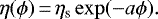
Gravitational forcing during Io’s orbit around Jupiter varies periodically due to its eccentricity. The materials that compose its interior deform in response to these periodic fluctuations. The way the materials respond to this forcing depends on their mechanical properties. At Io’s tidal forcing period (1.769 days), its interior behaves like a viscoelastic body. The simplest viscoelastic model is the Maxwell solid, which consists of an elastic element and a viscous element combined in series, characterized by the elastic shear modulus μ and the shear viscosity η, respectively. For a forcing period close to the Maxwell time, defined as the ratio of the shear viscosity to the shear modulus, τM = η∕μ, the Maxwell rheology is a good approximation, but it fails to reproduce correctly the dissipation function for periods much smaller than typical tidal forcing periods of close-in moons (a few days) (e.g., Castillo-Rogez et al. 2011; Efroimsky 2012). Laboratory studies dedicated to the characterization of the periodic deformation of silicates at periods suitable for tidal forcing (e.g., Jackson et al. 2004; Faul & Jackson 2007; Sundberg & Cooper 2010) indicate that alternative rheology models, such as the Andrade model (Castillo-Rogez et al. 2011; Efroimsky 2012; Bierson & Nimmo 2016) or the Sundberg-Cooper model (Sundberg & Cooper 2010; Renaud & Henning 2018) are more appropriate.
Due to experimental difficulties, very few studies have considered the attenuation behavior of partially molten rocks (Jackson et al. 2004). As a result, the rheological parameters on which the Andrade and Sundberg-Cooper models are based cannot be derived. The simplest approach to describe the viscoelastic behavior of partially molten rocks is to consider a Maxwell model, using the elastic modulus and viscosity values that has been widely studied in the literature dedicated to these rocks (Sect. 2.3). For partially molten rocks containing a high melt fraction (>10%), the estimated range for Maxwell times (from hundreds of days to a few minutes) is relatively close to Io’s tidal period, so that the Maxwell model provides a reasonable estimate of the dissipation rate.
In this study we adopt a Maxwell rheology for layers where a significant fraction of melt (> 25%) is present (subsurface and/or bottom molten layers) and an Andrade rheology for the other layers (crust and mantle excluding the partially molten layers).
2.3 Rheology of partially molten rocks
The partial melting of Io’s mantle rocks necessarily occurs at depth, albeit for partly unconstrained temperature and pressure conditions. The presence of magma severely alters the rheological properties of the whole rock. At low melt fractions the material is best described as a solid matrix with fluid pores (e.g., Schmeling et al. 2012). Its deformation is dominated by solid-state rheology. Atlarge melt fractions (or low crystal fractions), the material loses shear strength and tends to behave like a fluid. This led to the concept of a rheological critical melt fraction (RCMF) associated with a sharp transition from the solid behavior to the liquid behavior (e.g., Renner et al. 2000).
In the context of the present study, focused on solid-body tides, we consider melt fractions up to the RCMF and slightly above in order to mimic the significant drop in strength. In practice, most theoretical and experimental studies devoted to the effect of partial melts on the rheology of rocks focus on viscosity as this parameter plays a prominent role in the dynamics. Following the pioneering work of Arzi (1978), suggesting a threshold value of about 25–30% for RCMF, several studies reported a wide range of values, from 26 to 62% (e.g., Van der Molen & Paterson 1979; Bulau et al. 1979; Vigneresse et al. 1996; Renner et al. 2000; Scott & Kohlstedt 2006; Caricchi et al. 2007; Costa et al. 2009). The width of the transition is also not well constrained by these studies.
On the solid-state side of the rheological transition, experimental work focused on the deformation of partially molten materials in the laboratory for melt fractions up to 40% (e.g., Cooper & Kohlstedt 1986; Hirth & Kohlstedt 1995b,a; Lejeune & Richet 1995; Kohlstedt & Zimmerman 1996; Scott & Kohlstedt 2006). Empirical laws have been proposed to parameterize these results. A second approach is to derive theoretical models of the microscale physics and produce rheological laws suitable for use on planetary scales (e.g., Cooper et al. 1989; Takei & Holtzman 2009; Schmeling et al. 2012; Rudge 2018). All these studies indicate an exponential decrease in viscosity as a function of melt fraction.
Unlike viscosity, the elastic properties of partially molten rocks are studied only for small values of the melt fraction (typically a few percent), probably due to a lack of prior community need. On Earth this is indeed motivated by the existence of the asthenosphere, which is supposed to involve only a small amount of partial melts. Theoretical models were developed to describe the effect of melt fraction on the shear and bulk modulus (e.g., Walsh 1968, 1969; O’Connell & Budiansky 1977; Mavko 1980; Schmeling 1985). These models quantify the dependence of seismic wave speeds and attenuation upon melt fraction and fluid-filled inclusions of specified shape (e.g., ellipsoids, grain-boundary films, or grain-edge tubes). The viscoelastic behavior of partially molten rock is also investigated in the laboratory through forced torsional oscillation (Berckhemer et al. 1982; Bagdassarov & Dingwell 1993). To our knowledge, no experimental work has been done on the elastic moduli for melt fractions approaching and exceeding the RCMF. For this reason results obtained at low melt fractions have to be extrapolated to higher values to describe the elastic behavior up to the RCMF transition. Above RCMF we assume a mathematical description similar to viscosity for which experimental constraints exist (Costa et al. 2009).
3 Method
In this section we detail the methods and model assumptions considered for the internal structure (Sect. 3.1), the rheological laws used to describe the influence of melt fraction on the viscous and elastic parameters (Sect. 3.2), and the computation of the viscoelastic deformation of Io’s interior (Sects. 3.3 and 3.4).
Physical and orbital characteristics of Io.
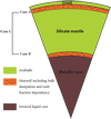 |
Fig. 1 Model of Io’s internal structure used for the computations. The considered rheology can be divided into three groups: (1) the solid mantle and crust, described by an Andrade rheology neglecting bulk dissipation; (2) the partially molten layers, either beneath the crust (case A) or at the core mantle boundary (case B), or a combination of both (Case C), described by a Maxwell rheology including both shear and bulk dissipation and accounting for the effect of melt on the viscoelastic parameters (following the rheological law described in Sect. 3.2); (3) the inviscid liquid metallic core. |
3.1 Properties of Io’s interior structure
The internal structure of Io is constrained from the mean density, mean radius, and moment of inertia (Table 1), deducedfrom the Galileo gravity data (Anderson et al. 2001; Sohl et al. 2002). The interior model consists of (moving from surface to center) a silicate crust, a silicate mantle, and a liquid metallic core (Fig. 1). The density of each layer is assumed to be uniform (see Table 2).
Estimates of the thickness of Io’s crust are uncertain. The only direct constraints come from lithospheric support of mountain ranges (Schenk et al. 2001), suggesting a lower limit of 20 km (e.g., Carr et al. 1998). We set the crustal thickness to 30 km, with a density of 3000 kg m−3. The core radius is given as 955 km (thus a mantle thickness of 836.6 km), providing reasonable values for the densities of the silicate mantle and metallic core satisfying the observed mass and moment of inertia. Core density is 5165 kg m−3 in agreement with the eutectic Fe-FeS composition (~5150 kg m−3, Usselman 1975; Anderson et al. 1996). The mantle density is 3263 kg m−3, similar to Earth’s olivine-rich upper mantle (3300 kg m−3, Dziewonski & Anderson 1981). As will be discussed later, changing the crustal thickness, core size, and mantle densities over reasonable ranges of values does not significantly change the results that are presented in this study.
As noted above, the presence of a partially molten layer beneath the crust in the upper part of Io’s mantle is a long-standing hypothesis in the literature (e.g., Segatz et al. 1988; Ross et al. 1990; Khurana et al. 2011). The melt content and thickness of this layer is a matter of debate, however. Proposed thickness values range between 50 and 200 km, which we adopt as a range for this parameter for both top and bottom molten layers. The melt fraction is varied between 25% and values slightly above the RCMF (Sect. 3.2).
For the sake of completeness, we also investigate the influence of a partially molten layer at the base of Io’s mantle, not accessed by magnetic sounding but indicated as a possibility in some convection models dedicated to Io’s mantle (Monnereau & Dubuffet 2002). Three configurations are considered: one with a top partially molten layer (case A), one with a bottom partially molten layer (case B), and one with both top and bottom partially molten layers (case C).
A reference value of 100 TW for the tidally dissipated power is chosen to represent Io’s heat budget. It should be noted that this value, selected in order to quantify the role of bulk dissipation compared to a reference state, is far from certain, and the typical variability range is between 65 and 125 TW (e.g., Lainey et al. 2009). This choice is discussed further in Sect. 5.
Density, rheological solid-state parameters, and interior structure characteristics assumed for Io’s interior.
3.2 Rheology of partially molten layers
Here we describe the effect of melt fraction ϕ on the four viscoelastic parameters used to describe the rheology of the partially molten layers: (shear) viscosity η, bulk viscosity ζ, shear modulus μ, and bulk modulus K. This is displayed in Fig. 2.
A single relationship defined for the whole melt range
In the following we restrict our investigation to a range of melt fraction values around the RCMF, shown as a shaded rectangle in Fig. 2. The choice of the minimum value for melt fraction ϕ is motivated by a weak dissipation for values smaller than ϕ = 0.25. The choice of themaximum value ϕ = 0.33 is dictated by numerical limitations. As is shown below, for all cases investigated this range enables us to capture the reference value of 100 TW for the tidally dissipated power. We note that for larger values of ϕ, not accessed by our numerical procedure, the rheological parameters η, μ, and K approach the much lower values associated with the liquid phase, albeit in a very uncertain way; in this domain the dissipation mechanisms envisioned in our viscoelastic formalism, which essentially correspond to solid-body tides, are less pertinent as other mechanisms might contribute to the dissipated budget.
Since the rheological parameters are poorly constrained by experiments and theory in the RCMF range, we adopt the semi-empirical model developed by Costa et al. (2009) that proposes a single formalism to describe the shear viscosity η from the purely solid-state to the purely liquid-state. Notably, this formalism includes the strong decrease in η characterizing the transition from solid-state behavior to liquid-state behavior. Since this transition is not constrained for elastic parameters μ and K, we use the same formalism (which appears to be a physically reasonable assumption),
![Mathematical equation: \begin{equation*}\bullet(\phi)= \bullet_l \frac{1+\Theta^{\delta}}{[1-F(\Theta, \xi, \gamma)]^{B (1-\phi_*)}},\end{equation*}](/articles/aa/full_html/2021/06/aa39433-20/aa39433-20-eq3.png) (1)
(1)
where rheological parameter ∙ is the shear viscosity η, the shear modulus μ, or the bulk modulus K. Two auxiliary functions are introduced:
 (2)
(2)
![Mathematical equation: \begin{equation*}F\,{=}\,(1-\xi) { } erf \Bigg[\frac{\sqrt{\pi}}{2 (1-\xi)} \Theta (1+\Theta^{\gamma})\Bigg].\end{equation*}](/articles/aa/full_html/2021/06/aa39433-20/aa39433-20-eq5.png) (3)
(3)
Except for parameter B, the Einstein coefficient (which is set to 2.5), all other parameters are tuned to reproduce the available constraints on the specific rheological parameter, from the solid-state endmember ∙s to the fully liquid-state endmember ∙l. The chosen solid- and liquid-state parameters of reference for the viscosity, shear modulus, and bulk modulus are described below. The values of δ, ξ, γ, and ϕ* also depend on the specific rheological parameters considered; they are listed in Table 3.
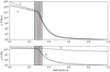 |
Fig. 2 Effect of melt fraction ϕ on the viscoelastic parameters: shear viscosity η and modulusμ (solid lines), bulk viscosity ζ and modulusK (dash-dotted lines). The red vertical dashed line denotes the rheological critical melt fraction (ϕc) where the transition between solid-state and liquid-state behaviors occurs. The shaded rectangle illustrates the restriction of our investigation to a range of melt fraction values around the RCMF. |
Solid-state end-member ∙s
The solid-state viscosity of mantle rocks ηs is uniform throughout the mantle. It is set to 1019 Pa s (Table 2), consistent with the typical value expected for dry olivine-dominated rocks near their melting point (e.g., Karato & Wu 1993). The solid-state shear and bulk modulus, μs and Ks of the mantle are set to 60 and 200 GPa, respectively (Table 2). We note that the effect of temperature and pressure change with depth on the silicate bulk modulus is only moderate: values typically range between 150 and 250 GPa forIo’s mantle pressure conditions (e.g., Jackson 1998). Our results are generally insensitive to this value.
Liquid-state end-member ∙l
The shear viscosity of the melt phase ηl is set to 1 Pa s, a typical value for basaltic melts (e.g., Shaw et al. 1968). Ultrasonic velocity measurement indicate that the bulk modulus of basaltic melts is one order of magnitude lower than those of expected mantle minerals, ranging between 1 and 30 GPa. These bulk moduli have been measured on silicate magma types ranging from basalt to silica-rich synthetic and natural compositions, all exhibiting the same decrease from the solid-state value. We use here a value of Kl = 1 GPa, as suggested by Stolper et al. (1981), Murase & McBirney (1973), and Rivers & Carmichael (1987). Varying K of 1 GPa and 30 GPa in our calculations has only a minor effect on the results. We note that while the shear modulus is expected to be zero for a liquid, we use a (non-zero) small value (μl = 10 Pa), for numerical reasons. We performed tests for μl values five orders of magnitude smaller and larger than our reference value, keeping the same value for μs. As we focused on ϕ values near the transition value ϕc (described below), these tests showed that the value assumed at ϕ = 1 does not impact the results displayed in the present study.
Rheological critical melt fraction (ϕc)
As noted in Sect. 2.3, a transition occurs at the rheological critical melt fraction (ϕc) between two main regimes of deformation: solid-dominated behavior (0 < ϕ < ϕc) and liquid-dominated behavior (ϕc < ϕ < 1). In Fig. 2 this corresponds to a dramatic rupture of the slope in the relationship introduced by Costa et al. (2009). Given the values of the rheological parameter for the liquid ∙l and solid ∙s phases, the location of ϕc is controlled by parameter ϕ* in Eqs. (1)–(3), which differs for η, μ, and K. For the results presented hereafter, we set the value of ϕc to 0.3. We also tested values ranging between 0.25 and 0.4; this does not induce significant changes to the main behavior presented here. What matters is not the exact value of ϕc, but the difference between the value of ϕ considered in the partially molten layer and the threshold value ϕc.
Transition to the liquid-state behavior above ϕc
For sufficiently large melt fractions (or sufficiently small crystal fractions), it is commonly assumed in the literature that the viscosity of the partially molten material increases with the crystal fraction. The classical exponential relationship proposed by Roscoe (1952) introduces a drastic increase in viscosity as ϕ decreases toward ϕc; this is embedded in the formalism of Costa et al. (2009) used in this study.
The width of this transition is controlled by the parameter γ (Eqs. (1) and (3)). In the absence of further constraints, γ is set to 5, as in Costa et al. (2009). Some studies considered arbitrarily a much sharper decrease in the shear modulus μ at the rheological transition (e.g., Fischer & Spohn 1990; Moore 2001). We have conducted tests with such a sharp decrease, although this has no rheological justification. Results indicate a significant increase in bulk dissipation. We thus consider that adopting the same formalism for η and μ (Eqs. (1)–(3)) leads to a conservative estimate of the role of bulk dissipation. The parameter ξ (Eqs. (1) and (3)) is chosen to mimic the appropriate decrease in strength as the melt fraction increases. For ϕ <ϕc, the effect of melt fraction ϕ on these elastic parameters is moderate. The constraints used to define the slope of curves for ϕ <ϕc (parameter δ in Eq. (1)) are described in Appendix A.
Bulk viscosity
In the framework of two-phase flow, the full description of an isotropic linear medium requires the use of two viscosities, a bulk viscosity ζ and a shear viscosity η (McKenzie 1984; Scott & Stevenson 1986; Ricard et al. 2001). Bulk viscosity describes the rate of volume change of the material. Although more work was devoted to viscosity than to any other rheological property of silicate melts, no measurements exist for the bulk viscosity of natural or analog systems applicable to the crust or mantle. As a consequence, in large-scale geodynamic models, bulk viscosity is usually described by a simplified law proportional to η∕ϕ based on theoretical considerations (e.g., Ricard et al. 2001; Simpson et al. 2010; Schmeling et al. 2012). In the absence of constraints, we adopt this simplified relationship:
 (4)
(4)
As shown in Fig. 2, this formalism superimposes an increase in the bulk viscosity ζ at low melt fraction ϕ, while preserving the rheological transition embedded in η (Eqs. (1)–(3), ζ is plotted for ϕ > 0.01 in Fig. 2).
3.3 Tidal dissipation including bulk dissipation
The constitutive equation for a Maxwell rheology is rewritten, including bulk dissipation, in order to take it into account in the calculation of tidal dissipation in Io’s partially molten layers. For a Maxwell compressible medium with no bulk dissipation, the constitutional relationship between stress and strain tensors is (e.g., Peltier 1974)
 (5)
(5)
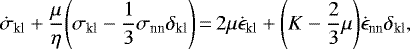
where σkl and ϵkl are the stress and strain tensor elements, respectively, and δkl is the Kronecker symbol. Following the convention, repeated indices imply summation. The point above the variables represents a derivative with respect to time. Bulk dissipation can be considered by adding a term taking into account bulk viscosity ζ:
 (6)
(6)
In the Fourier domain, the constitutive relationship becomes
 (7)
(7)
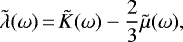
where ω is the frequency, and the tilde (~) indicates Fourier transform. According to the correspondence principle, this corresponds to a generalized Hooke’s law with complex moduli  ,
,  , and
, and  written as
 (8)
(8)
 (9)
(9)
 (10)
(10)
3.4 Computation of tidal dissipation
The viscoelastic deformation of Io under the action of periodic tidal forces is computed following the method of Tobie et al. (2005, 2019). A novel step is taken with the inclusion of bulk dissipation in addition to shear dissipation in the calculation (Sect. 3.3). The only difference relative to the approach of Tobie et al. (2005) is the consideration of a non-zero imaginary part for the complex bulk modulus, as defined in Eq. (10).
The tidal response of Io’s interior is computed by integrating the radial and tangential displacements (y1 and y3, respectively), the radial and tangential stresses (y2 and y4) and the gravitational potential (y5), as defined by Takeuchi & Saito (1972). The full set of equations, the boundary conditions (center, liquid-solid interface, surface), and the numerical scheme to solve them in detail are provided in Appendix B.
The complex Love number k2 is determined from the radial functions y5 (Rs) at the moon surface. The global dissipated power is determined by the imaginary part of the Love number, Im(k2) and the orbit characteristics (Table 1). For a synchronously rotating body in an eccentric orbit, the global dissipated power is
 (11)
(11)
(e.g., Segatz et al. 1988) with ω the angular orbital frequency (ω = 2π∕T), T being the orbital and rotational period, Rs the radius of thesatellite, G the gravitational constant, and e the orbital eccentricity. This formulation to the first order in eccentricity in the tidal potential (Eq. (B.7)) is valid for low eccentricity (<5%, Wisdom 2008; Běhounková et al. 2011), and is therefore applicable to Io.
The radial distribution of the tidal dissipation rate, taking into account both shear and bulk dissipations, can be determined for the radial sensitivity functions to shear and bulk moduli, Hμ and HK, introduced by Tobie et al. (2005):
 (12)
(12)
Here Hμ and HK are determined from the radial functions y1, y2, y3, and y4 (see Eq. (33) in Tobie et al. 2005, and our Appendix C for more details). Im (μ) and Im (K) are the imaginary part of the complex shear modulus and bulk modulus, respectively. The only difference relative to the approach of Tobie et al. (2005) is the consideration of a non-zero Im (K) term in the partially molten layer.
The local tidal heating rate per unit of volume averaged over one cycle is evaluated at any point inside the body from the complexstress and strain tensors, determined from the radial functions (see Appendix D):
 (13)
(13)
By integrating radially the volumetric heating rate Htide over a given layer, for instance the partially molten layer, we then derive the tidal heat flux qtide, which is then used to discuss the tidal heat pattern. From the complex Love number we can assess the total dissipated power using Eq. (11), while the two formulas in Eqs. (12) and (13) provide information on the radial distribution and the spatial pattern of dissipation, respectively.
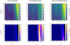 |
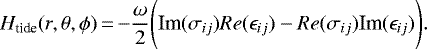
Fig. 3 Io’s tidal heat budget as a function of melt fraction ϕ and the thickness dmelt of the partially molten layer(s). Three configurations are considered for the internal structure (see Fig. 1): with one partially molten layer at the top (case A, left column) or at the bottom of the mantle (case B, middle column), or with partially molten layers both at the top and bottom of the mantle (case C, right column). The color scale refers to the global tidal power Pbulk, including the contribution of bulk dissipation (top panel), and to the ratio (Pbulk − Pnobulk)∕Pnobulk, with Pnobulk designating the reference global tidal power produced with shear dissipation only (bottom panel). The red curves highlight the 100 TW value. The black curve indicates the parameters required to obtain this same value without bulk dissipation. For each configuration the red star denotes a reference case corresponding to a thickness dmelt = 100 km. The white dashed line indicates the value of ϕc. |
4 Results
4.1 Influence of bulk dissipation on tidal heat budget
The top panel of Fig. 3 displays the global tidal power Pbulk in Io’s interior as a function of the characteristics of the partially molten layer(s), melt fraction ϕ and thickness dmelt. Over the range of values considered for ϕ and dmelt, several tens of TW can be generated, whatever the internal structure configuration (cases A, B, or C; see Fig. 1). For a given thickness of the partially molten layer dmelt, increasing the melt fraction ϕ first results in an increase in Pbulk. Below the critical melt fraction (ϕc = 0.3), however, the tidal power never reaches 100 TW. A drastic increase in the tidal power is observed beyond the critical melt fraction. Typical values of hundreds of terawatts are observed for ϕ in the range 0.3–0.33. Ultimately, if the melt fraction ϕ keeps increasing, the decrease in η, ζ, K, and μ leads to a decrease in Pbulk. This is particularly visible in the case of a bottom layer (Fig. 3, case B), where the maximum value of Pbulk is observed at ϕ≃ 0.316 and dmelt = 200 km. For the case involving a partially molten layer at the top of the mantle (Fig. 3, case A) this maximum occurs at larger values of ϕ (> 0.32 for dmelt = 200 km, larger valuesof ϕ for thinner layers). For the configuration where bottom and top partially molten layers are introduced that surround the solid-state mantle (Fig. 3, case C), the maximum value of Pbulk is obtained for ϕ values in excess of 0.33 that do not appear in the figure.
The top panel of Fig. 3 also indicates the melt layer characteristics for which Io’s estimated heat output (for which we take as a reference value 100 TW) can be reproduced for solutions with bulk dissipation (red isolines) and without bulk dissipation (black isolines). For a top molten layer, owing to dissipation enhancement associated with bulk dissipation, 100 TW is reached for a melt content smaller of 0.003 than for the case with no bulk dissipation. For a bottom molten layer, the produced tidal power never reaches 100 TW in the absence of bulk dissipation, which explains the absence of black isoline in Case B. Once bulk dissipation is considered, 100 TW can be generated for a melt content comprised between ~ 0.31 and ~ 0.32.
The bottom panel of Fig. 3 illustrates the morphology of the dissipation by comparing the tidal power produced when both bulk and shear dissipation are considered (Pbulk) to the reference tidal power that is produced when only shear dissipation is considered (Pnobulk). As noted above, tidal heating is especially enhanced by the addition of bulk dissipation just above ϕc, with a maximum enhancement for ϕ = 0.312. The thinner the partially molten layer, the greater the enhancement of tidal heating for this melt fraction, whatever the location of the partially molten layer. The maximum enhancement is observed for the bottom layer configuration. On the contrary, above ϕ = 0.32, considering shear dissipation only leads to an overestimation of the tidal heat budget (Pnobulk > Pbulk).
As illustrated in Fig. 4 (for partially molten layers 100 km in thickness), the global power with or without bulk dissipation is comparable as long as ϕ < ϕc (0.3 in this study). When ϕ approches and exceeds ϕc, the two solutions with or without bulk dissipation diverge. This is particularly evident in the case of a bottom layer (Case B, green curves) where the total power decreases with increasing melt fraction in the absence of bulk dissipation, while it strongly increases with bulk dissipation. The case of a top layer (Case A, red curves) is somewhat different: when ϕ exceeds ϕc, both solutions with or without bulk lead to an increase in dissipation. The solution with bulk dissipation increases initially faster, but becomes less dissipative than the no-bulk solution for ϕ exceeding 0.32. This observation is also valid for Case C (blue curves).
Figure 5 shows the radial distribution of tidal dissipation rate  (Eq. (12)) for the three interior models, in the case where Pbulk = 100 TW (red stars in Fig. 3). When bulk dissipation is considered (solid lines), the tidal power is increased in the partially molten layers. The value of
  is higher than 6 × 10⁻⁶ W m−3 in the top layer and 3 × 10⁻⁵ W m−3 in the bottom layer, one to two orders of magnitude higher than in the solid mantle adjacent to the partially molten layer.
These profiles highlight the enhancement associated with the introduction of bulk dissipation already observed in Figs. 3 and 4. When a partially molten layer is introduced on top of the mantle (cases A and C), the dissipation enhancement is highest in the middle of the layer (compare red and blue, solid and dash-dotted lines at R ≃ 1750 km). In the configurations with a bottom layer (cases B and C), the introduction of bulk dissipation leads to higher heating rates than in the solid mantle immediately above, while dissipation heating is lower when bulk dissipation is not accounted for, as noted in Fig. 4 (compare blue and green, solid and dash-dotted lines in the bottom 100 km thick layer). Comparison with solutions considering a fully solid core clearly indicates that the two-orders-of-magnitude effect for Case B when including bulk dissipation (bottom panel of Fig. 5) is explained by the boundary condition imposed by the presence of the liquid core at the base of the partially molten layer, which results in different stress conditions at the bottom interface.
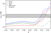 |
Fig. 4 Io’s tidal heat budget Pglob as a function of melt fraction of the partially molten layer. Configurations for the interior structure involve: a top partially molten layer (case A, red), a bottom partially molten layer (case B, green), and a combination of the two, both layers being of equal thickness (case C, blue). The layers thickness is dmelt = 100 km. Cases involving bulk dissipation correspond to solid curves. Cases where bulk dissipation is not included correspond to dash-dotted curves. The shaded rectangle gives Io’s heat budget range (65–125 TW; see, e.g., Lainey et al. 2009). |
 |
Fig. 5 Radial distribution of the tidal dissipation rate |

4.2 Tidal dissipation pattern including bulk dissipation
Figures 6 and 7 display the tidal heat flux qtide computed by radially integrating the volumetric tidal heating Htide (Eq. (13)) throughout the dissipative molten layer in the reference models for cases A (top) and B (bottom) indicated by red stars in Fig. 3. The left panels correspond to the computation of tidal heat including bulk dissipation and the global value of Pbulk (integration of qtide over the whole surface area), and thus amounts to 100 TW. The right panels correspond to computations with a similar melt configuration, but when bulk dissipation is not accounted for. The value of Htide is much lower in the latter case. Below, we focus on the dissipation pattern, and thus on lateral variations in qtide rather than on the absolute values.
The degree-two shape of the tidal potential results in a modulation of tidal heating as a function of latitude and longitude. The introduction of bulk dissipation alters the dissipation pattern in both configurations. When the partially molten layer is located at the top of the mantle (Case A, Fig. 6), the computation with no bulk dissipation (right panel) yields the classical pattern of Io’s near surface partially molten layer (e.g., Segatz et al. 1988; Hamilton et al. 2013; Steinke et al. 2020): four local maxima at low latitudes; two absolute maxima at longitudes 0 and 180°, corresponding to the sub- and anti-Jovian points; and two secondary maxima at longitudes 90 and 270°, corresponding to the leading and trailing meridians. The maximum tidal heat production occurs at 30° latitude, north and south of the sub- and anti-Jovian points. The pattern obtained when bulk dissipation is introduced (left panel) also results in maxima at low latitudes, but with longitudinal variations different from the classicalpattern. The leading and trailing meridians systematically correspond to minimum values of qtide at all latitudes. At the equator, these minima correspond to half the value at the sub- and anti-Jovian points, now corresponding to the absolute maxima of the tidal power. More dissipation is produced at high latitudes (>45°), with values at the poles never less than 25% of the maximum value.
As noted above, the configuration with a bottom partially molten layer (Case B, Fig. 7) is extremely affected by the introduction of bulk dissipation (cf. Fig. 5). Without bulk dissipation, the tidal power is strongly inhibited in this region, as indicated by the very low value of qtide, while with bulk dissipation, it is strongly enhanced. It is worth noting that the pattern with bulk dissipation (Fig. 7, left), is similar to that observed when the partially molten is at the top (Fig. 6, left) (i.e., qtide is maximum at low latitudes). As a consequence, discriminating between a top or a bottom partially molten layer seems difficult on the sole basis of the dissipation pattern. Slight modulations are observed, however: the minima at the leading and trailing meridians (90 and 270°) are less pronounced, and four maxima are located at intermediate longitudes between these meridians and those of the sub- and anti-Jovian points. For the case that does not include bulk dissipation (Fig. 7, right), the pattern also resembles that of case A (Fig. 6, right) (i.e., corresponding to the classical pattern of Io’s near surface partially molten layer).
While dissipation patterns do not change significantly depending on the location of the layer, the inclusion of bulk dissipation has a major effect compared to when shear dissipation alone is considered. Dissipation patterns are controlled by the different components of the stress and strain tensors. As shown in Fig. D.1, the dissipation pattern of the top partially molten layer is mainly controlled by the three radial components σrr ϵrr, σrϕ ϵrϕ, and σrθ ϵrθ, with a stronger contribution of the σrrϵrr component when bulk dissipation is included compared to the solution without bulk dissipation (six times higher). The resulting pattern (Fig. 6, left) is a modulation of the σrr ϵrr, σrϕ ϵrϕ, and σrθ ϵrθ patterns. The dissipation pattern of the bottom layer including bulk dissipation is completely dominated by the radial component σrr ϵrr, 30 times higher than the equivalent computation with no bulk dissipation (see Fig. D.1).
Changing the parameters that control the rheological transition at the RCMF (Eqs. (1)–(3)) and the asymptotic elastic value for the fully liquid state (μl and Kl) has a minor effect on the resulting dissipation pattern. The patterns displayed in Figs. 6 and 7 are representative of Case A and B and are mostly determined by the depth and thickness of the assumed molten layer.
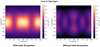 |
Fig. 6 Patterns of tidal heat flux qtide integrated over the top partially molten layer for one orbit cycle at a given location for the reference model denoted by a red star in Fig. 3, Case A, corresponding to ϕ = 0.3122. Left: values obtained when bulk dissipation is accounted for (providing a total power Pbulk = 100 TW). Right:values obtained when bulk dissipation is not accounted for; in this case the total power is less than 100 TW (45 TW). The same scale is used to highlight the tidal power enhancement due to bulk dissipation. |
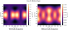 |
Fig. 7 Patterns of tidal heat flux qtide integratedover the bottom partially molten layer for one orbit cycle at a given location for the reference model denoted by a red star in Fig. 3, Case B, corresponding to ϕ = 0.3106. Left: values obtained when bulk dissipation is accounted for (providing a total power Pbulk = 100 TW). Right:values obtained when bulk dissipation is not accounted for; in this case the total power is less than 100 TW (12 TW). The two color scales are not the same. |
5 Discussion and conclusion
In the present study we investigated the solid-body tides of partially molten interiors and quantify the potential role of bulk dissipation. We chose Io as the archetype of a planetary body where tidal heating is the key driver of interior evolution and magmatic activity. Classical models are revisited along two lines: (1) bulk attenuation is accounted for in the computation of tidal dissipation and (2) rheological laws for viscous and elastic parameters describe the influence of partial melts from zero melt present up to beyond the critical value associated with the rheological transition to liquid-state behavior.
Bulk dissipation starts to contribute significantly for melt fractions approaching the value corresponding to the rheological transition, termed RCMF. A total power of typically 100 TW, required to explain Io’s thermal budget, is reached only after a few percent above the RCMF. We note that for liquid-dominated materials, as would be the case for a magma ocean, our modeling approach is not valid anymore. While the rheological parameterization we use describes the variation of rheological parameters over the full range of melt fraction (from 0 to 1), our numerical approach becomes unstable when the shear modulus becomes smaller than ~ 106 Pa. Alternative formulations, such as the propagator matrix technique used in various studies dedicated to Io (e.g., Segatz et al. 1988; Renaud & Henning 2018), can handle smaller values of shear modulus. However, this formulation ignores compressibility, and therefore cannot be used to assess the role of bulk dissipation. For these reasons we limited our analysis to melt fractions below 0.33 (i.e., 3% above the RCMF value chosen here). As we showed that the produced tidal power rapidly diverges from the expected 100 TW, this appears to be a reasonable approach. This does not exclude that other solutions producing 100 TW for higher melt fraction exist, but such a case should be explored with an alternative modeling approach relying on fluid formulation of the problem rather than on a solid-based viscoelastic formulation,as used here. In addition, we should keep in mind that the reference value of 100 TW chosen in this study to quantify the role of bulk dissipation is associated with a significant uncertainty; the estimates typically vary between 65 and 125 TW (e.g., Lainey et al. 2009). Independently of the assumed total power, we show that bulk dissipation allows the production of several hundreds of terawatts in a local archetype present in our Solar System.
Our results show that a strong increase in tidal dissipation occurs in partially molten layers when the melt fraction exceeds the critical melt fraction, estimated between ~0.25 and 0.40. All the results presented here assumed a critical value of 0.30, but similar behavior is observed when considering different values. Moreover, we show that once above this critical value, tidal dissipation is enhanced in many circumstances, and reduced in some others, by bulk dissipation. Below the critical value, the effect of bulk dissipation remains negligible. In the case of a subsurface partially molten layer located beneath the crust (asthenosphere), this effect is greatest for thin layers (~50 km): up to four times the value without bulk dissipation. For a partially molten layer located at the base of the solid-state mantle, we show that neglecting bulk dissipation completely changes the results. When bulk dissipation is not taken into account, calculations show a strong decrease in tidal heating in such a layer, while our results demonstratethat a strong increase is expected instead. The two differ typically by more than three orders of magnitude.
Our results imply that, given all other assumptions and parameter choices of the tests we performed, partially molten layers within Io (either on the top or bottom of the mantle) should have a melt fraction above the RCMF value (>0.25–0.40) in order to match Io’s heat output (~100 TW). This differs from the results of Bierson & Nimmo (2016), who find solutions matching the total heat output for melt fraction below the RCMF value, ranging between 0 and 0.25. This discrepancy comes from the different values of rheological parameters for the solid matrix. As noted by Bierson & Nimmo (2016), the solutions depend on the assumed rheological parameters, which are poorly experimentally constrained for partially molten rocks. As the main objective of the study is to test the effect of including bulk dissipation, we deliberately chose to prescribe the rheological parameters for the solid matrix (ηs = 1019 Pa s) and consider a Maxwell rheology for the partially molten layer, in the absence of constraints to derive the rheological parameters for an Andrade model. The influence of the solid matrix rheology on the total heat budget of Io will be addressed in a forthcoming study.
Including bulk dissipation also severely modifies the tidal dissipation pattern. For a partially molten layer located on top of the solid-state mantle, maximum tidal heating is observed at low latitudes, as in the case when bulk dissipation is not accounted for. However, tidal heating is non-zero at the poles (25% of the maximum value) contrary to calculations without bulk dissipation. This feature may explain the observed volcanism at high latitudes on Io (e.g., Veeder et al. 2012; Davies et al. 2015) in addition to the apparent concentration of volcanic landforms around the equator (Kirchoff et al. 2011; Hamilton et al. 2013). Furthermore, while the classical pattern (i.e., without bulk dissipation) displays local maxima at the leading and trailing meridians (e.g., Segatz et al. 1988; Beuthe 2013; Steinke et al. 2020), these meridians correspond to minima when bulk dissipation is included. These modulations are mild, however, and might be difficult to discriminate on the basis of Io’s volcanism. Moreover, it is argued in the literature that deep mantle heating on Io leads to an inverse pattern when compared to a shallower heat source associated with a low-viscosity layer, with maxima located at high latitudes. We show that when bulk dissipation is included, a deep partially molten layer at the base of the mantle instead yields a pattern that is roughly similar to that of an asthenosphere (i.e., maxima are located at low latitudes). Our results demonstrate that bulk dissipation is a crucial process when predicting dissipation in partially molten layers, such as the asthenosphere of Io.
While Spencer et al. (2020) argue that a partially molten layer at the base of Io’s mantle might not be the most physically plausible on the basis of two-phase flow, Monnereau & Dubuffet (2002) suggested that a significant amount of melt may be present at the base of the mantle depending on the efficiency of heat transfer through the mantle. However, based on existing observational and theoretical constraints we cannot determine which of the three cases tested (the top or bottom partially molten layer, or a combination of both) would be more likely. Furthermore this configuration might be of interest in other applications. A basal magma ocean has been proposed as possible on Earth over a long period of time (Labrosse et al. 2007). This can also be the case for Earth-sized exoplanets, hot molten likely bodies being common in exoplanetary systems (Henning et al. 2018). As an example, the TRAPPIST-1 system exhibits two planets (TRAPPIST-1 b and c) where tidal dissipation is expected to be the primary internal heat source (Barr et al. 2018; Turbet et al. 2018). Especially on TRAPPIST-1 b, the tidal heat flux estimated to be more than a few W m−2 (Turbet et al. 2018) would likely result in a large melt production in the interior and associated magmatic processes. Evaluating the heat production including bulk dissipation in partially molten layers is essential to understand the impact of tidal friction on such rocky exoplanets. Highly volcanic exoplanets, which can be variously characterized as “lava worlds”, “magma ocean worlds”, or “super-Ios”, are high-priority targets for investigation (Henning et al. 2018). Owing to their bright infrared flux and short orbital periods, they may be among the most detectable and characterizable low-mass exoplanets in the coming decade (Bonati et al. 2019). Io thus provides a local archetype of a diverse category of related silicate worlds with intense tidally driven volcanism (Barnes et al. 2010). Results of the upcoming observational facilities such as the Atmospheric Remote-sensing Infrared Exoplanet Large-survey (ARIEL) and the James Webb Space Telescope (JWST) must be examined in the light of our findings on the role of bulk dissipation.
Acknowledgements
The authors are grateful to the referee for a very detailed and constructive review which clearly improved the manuscript. This research received funding from the French “Agence Nationale de Recherche” ANR (OASIS project, ANR-16-CE31-0023-01) and from CNES for the preparation of the ESA JUICE and NASA Europa Clipper missions. M.B. acknowledges Czech Science Foundation grant no. 19-10809S.
Appendix A Constraints on rheological parameters at melt fractions ϕ <ϕc
For melt fractions beneath the rheological transition (ϕ < ϕc), shear viscosity η, shear modulus μ, and bulk modulus K are essentially described in our study by a power law whose slope is δ (Eq. (1)). The following constraints have been used to determine an appropriate value for this parameter.
The effect of a melt fraction ϕ on the viscosity of the solid matrix is typically described by an exponential decrease:
 (A.1)
(A.1)
Experimental studies on olivine valid up to a melt fraction ϕ = 0.25−0.3 report values for the exponential coefficient a in the range 26–32 (Mei et al. 2002; Kohlstedt et al. 2000; Scott & Kohlstedt 2006). A value of a = 30 is well described by δ = 25.7 (used in our computations; cf. Eq. (1)).
The moderate effect of melt fraction ϕ on elastic parameters can be described using the theoretical relationship derived by Mavko (1980) assuming the most appropriate melt geometry, namely interconnected tubes,
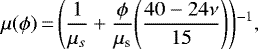 (A.2)
(A.2)
 (A.3)
(A.3)
where ν = 0.25 is the typical Poisson ratio for silicate rocks (e.g., Christensen 1996; Ji et al. 2018). In the formalism of Costa et al. (2009) used here (Eq. (1)), this corresponds to δ = 2.10 for μ and δ = 2.62 for K.
Appendix B Computation of the radial functions
B.1 Definition of the radial functions and overview of the differential equations
Tidal forcing by external bodies induces spheroidal modes of deformation inside the forced body. For a spherically symmetric interior model, the displacements u = (ur, uθ, uφ), the potential Ψ, and the stress components σij induced inside the body by the external tidal potential  can be expressed as the product between a radial part yi, which depends on the interior structure, and an angular part, which depends on the tidal potential exerted at the body surface,
  (Alterman et al. 1959; Takeuchi & Saito 1972):
 (B.1)
(B.1)
 (B.2)
(B.2)
 (B.3)
(B.3)
 (B.4)
(B.4)
 (B.5)
(B.5)
 (B.6)
(B.6)
It should be noted that the full expression of the different components of the stress and strain tensors is provided in Appendix D.
The five radial functions  depend on the radius (r); the radially dependent density, shear modulus, and bulk modulus (ρ, μ and K); and the forcing angular frequency (
 ), which may vary depending on the degree l and azimuthal order m of the forcing potential. In the particular case of a body in 1:1 spin-orbit resonance on an orbit with low eccentricity e, there is a single forcing frequency whatever the azimuthal order, which is equal to the mean motion or rotational angular frequency ω:
![Mathematical equation: \begin{eqnarray*}\Phi(R_{\textrm{s}}) &=& R_{\textrm{s}}{}\omega^{2}e \Bigg({-}\frac{3}{2}P_{2}^{0}(\cos\theta)\cos \omega t \nonumber \\&& + \frac{1}{4} P_{2}^{2}(\cos\theta)[3\cos \omega t \cos 2\varphi + 4 \sin \omega t \sin 2\varphi]\Bigg).\end{eqnarray*}](/articles/aa/full_html/2021/06/aa39433-20/aa39433-20-eq34.png) (B.7)
(B.7)
In addition to the five radial functions introduced above, a sixth radial function, y6, is used to account for the continuity of the gravitational potential gradient. It is defined so as to simplify the boundary conditions at the surface (Takeuchi & Saito 1972)
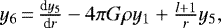 (B.8)
(B.8)
where G the universal gravitational constant.
By injecting these relationships in the Poisson equation
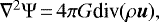 (B.9)
(B.9)
and in the equations of motions
![Mathematical equation: \begin{eqnarray*}\rho\frac{\partial^{2}\vec{u}}{\partial t^{2}} & = & \rho\vec{f}+(\textrm{div} \vec{\sigma}_{r},\textrm{div} \vec{\sigma}_{\theta}, \textrm{div} \vec{\sigma}_{\varphi}) \nonumber \\&& + \frac{1}{r}(-\sigma_{\theta\theta}-\sigma_{\varphi\varphi}, \sigma_{r\theta}-\sigma_{\varphi\varphi}\cot \theta,\sigma_{\varphi r}+\sigma_{\varphi\theta}\cot\theta),\nonumber \\[1pt]\end{eqnarray*}](/articles/aa/full_html/2021/06/aa39433-20/aa39433-20-eq37.png) (B.10)
(B.10)
with σr, σθ, and σφ representing the stresses exerted on the plane perpendicular to the axis ur, uθ and uφ, respectively,we obtain the following set of differential equations relating the six radial functions:
![Mathematical equation: \begin{equation*}\frac{\textrm{d}y_{1}}{\textrm{d}r}\,{=}\,\frac{1}{K+\frac{4}{3}\mu}\left\{y_{2}-\frac{K-\frac{2}{3}\mu}{r}[2y_1-l(l+1)y_3]\right\},\end{equation*}](/articles/aa/full_html/2021/06/aa39433-20/aa39433-20-eq38.png) (B.11)
(B.11)
![Mathematical equation: \begin{eqnarray*}\frac{\textrm{d}y_2}{\textrm{d}r} &=&-\omega_{lm}^{2}\rho y_1+\frac{2}{r}\left(\left(K-\frac{2}{3}\mu\right)\frac{\textrm{d}y_{1}}{\textrm{d}r}-y_2\right) \nonumber \\&& +\frac{1}{r}\left(\frac{2(K+\mu/3)}{r}-\rho g\right)[2y_1-l(l+1)y_3]\nonumber \\&& +\frac{l(l+1)}{r}y_4-\rho\left(y_6-\frac{n+1}{r}y_5+\frac{2g}{r}y_1\right),\end{eqnarray*}](/articles/aa/full_html/2021/06/aa39433-20/aa39433-20-eq39.png) (B.12)
(B.12)
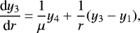 (B.13)
![Mathematical equation: \begin{eqnarray*}\frac{\textrm{d}y_4}{\textrm{d}r} &=& -\omega_{lm}^{2}\rho y_3-\frac{K-\frac{2}{3}\mu}{r}\frac{\textrm{d}y_{1}}{\textrm{d}r} \nonumber \\&& -\frac{K+\frac{4}{3}\mu}{r^2}[2y_1-l(l+1)y_3] \nonumber \\&&+\frac{2\mu}{r^2}(y_1-y_3)-\frac{3}{r}y_4-\frac{\rho}{r}(y_5-gy_1),\end{eqnarray*}](/articles/aa/full_html/2021/06/aa39433-20/aa39433-20-eq41.png) (B.14)
(B.14)
 (B.15)
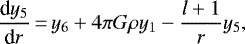
![Mathematical equation: \begin{equation*}\frac{\textrm{d}y_6}{\textrm{d}r}\,{=}\,\frac{l-1}{r}(y_6+4\pi G\rho y_1)+\frac{4\pi G\rho}{r}[2y_1-l(l+1)y_3].\end{equation*}](/articles/aa/full_html/2021/06/aa39433-20/aa39433-20-eq43.png) (B.16)
(B.16)
This system of differential equations has six independent solutions in general. However, the solutions can be rearranged in such a way that three of them are regular at r = 0. Each of these three sets of solutions (yi1, yi2, and yi3) can be integrated independently, as detailed in Appendix B.3. The full solution is a linear combination of these three solutions:  . The three constants A, B, and C are then determined by applying the appropriate boundary conditions at the surface.
B.2 Particular case of a liquid layer
The set of differential equations presented above is applicable only in solid internal layers. In liquid–fluid internal layers (μ = 0) there is no tangential stress (y4 = 0) and the differential equation dy3∕dr no longer exists, y3 becomes
![Mathematical equation: \begin{equation*}y_3\,{=}\,{-}\frac{1}{\omega^2\rho r}[y_2-\rho(gy_{1}-y_{5})],\end{equation*}](/articles/aa/full_html/2021/06/aa39433-20/aa39433-20-eq45.png) (B.17)
(B.17)
and the set of differential equations is reduced to
![Mathematical equation: \begin{equation*}\frac{\textrm{d}y_{1}}{\textrm{d}r}\,{=}\,\frac{1}{K}\left\{y_{2}-\frac{K}{r}[2y_1-l(l+1)y_3]\right\},\end{equation*}](/articles/aa/full_html/2021/06/aa39433-20/aa39433-20-eq46.png) (B.18)
(B.18)
![Mathematical equation: \begin{eqnarray*}\frac{\textrm{d}y_2}{\textrm{d}r} &=& -\omega_{lm}^{2}\rho y_1+\frac{2}{r}\left(K\frac{\textrm{d}y_{1}}{\textrm{d}r}-y_2\right) \nonumber\\&& +\frac{1}{r}\left(\frac{2K}{r}-\rho g\right)[2y_1-l(l+1)y_3] \nonumber \\&& -\rho\left(y_6-\frac{n+1}{r}y_5+\frac{2g}{r}y_1\right),\end{eqnarray*}](/articles/aa/full_html/2021/06/aa39433-20/aa39433-20-eq47.png) (B.19)
(B.19)
 (B.20)
![Mathematical equation: \begin{equation*}\frac{\textrm{d}y_6}{\textrm{d}r}\,{=}\,\frac{l-1}{r}(y_6+4\pi G\rho y_1)+\frac{4\pi G\rho}{r}[2y_1-l(l+1)y_3].\end{equation*}](/articles/aa/full_html/2021/06/aa39433-20/aa39433-20-eq49.png) (B.21)
(B.21)
For a liquid layer, the solutions to this differential equation system reduce to two independent sets of solutions: 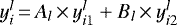 .
.
We note that y3 becomes indeterminate when ω → 0, so that a different solution should be adopted for very low frequencies, typically for tidal periods exceeding 5–10 days. At low frequency, the tidal response of a liquid layer can be approximated by a static equilibrium solution, as proposed by Saito (1974).
B.3 Solution integration and boundary conditions
Conditions at the center and initiation of integration
The set of differential equations is solved by integrating the independent solutions (two in liquid layers, three in solid layers) from the center to the surface. At the center, y1(0) = 0, y3 (0) = 0 and y5 (0) = 0. For initiating the integration at the first step, from R = 0 to R = dR, the three independent analytical solutions for a homogeneous sphere established by Pekeris & Jarosh (1958) and rearranged by Takeuchi & Saito (1972) are used.
A first solution is given by
 (B.22)
with
This solution is valid for both liquid and solid cases.
Two additional independent solutions are given by
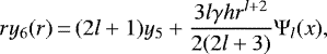
![Mathematical equation: \begin{equation*}ry_1(r)\,{=}\,-\frac{r^{l+2}}{l+3}\left[\frac{1}{2}lh\Psi_l(x)+f\Phi_{l+1}(x)\right],\end{equation*}](/articles/aa/full_html/2021/06/aa39433-20/aa39433-20-eq53.png) (B.23)
(B.23)
![Mathematical equation: \begin{eqnarray*}r^2y_2(r) &=& -(\lambda+2\mu)r^{l+2}f\Phi_l(x) \nonumber \\&& +\frac{\mu r^{l+2}}{2l+3} \left[-l(l-1)h\Psi_l(x)+2\left[2f+l(l+1)\right]\varphi_{l+1}(x)\right], \nonumber \\\end{eqnarray*}](/articles/aa/full_html/2021/06/aa39433-20/aa39433-20-eq54.png) (B.24)
(B.24)
![Mathematical equation: \begin{equation*}ry_3(r)\,{=}\,-\frac{r^{l+2}}{2l+3}\left[\frac{1}{2}h\Psi_l(x)-\Phi_{l+1}(x)\right],\end{equation*}](/articles/aa/full_html/2021/06/aa39433-20/aa39433-20-eq55.png) (B.25)
(B.25)
![Mathematical equation: \begin{equation*}r^2y_4(r)\,{=}\,\mu r^{l+2}\left\{\Phi_l(x)-\frac{1}{2l+3}\left[(l-1)h\Psi_l(x)+2(f+1)\Phi_{l+1}(x)\right]\right\},\end{equation*}](/articles/aa/full_html/2021/06/aa39433-20/aa39433-20-eq56.png) (B.26)
(B.26)
![Mathematical equation: \begin{equation*}y_5(r)\,{=}\,r^{l+2}\left[\frac{\alpha^2 f-(l+1)\beta^2}{r^2}-\frac{3\gamma f}{2(2l+3)}\Psi_l(x)\right],\end{equation*}](/articles/aa/full_html/2021/06/aa39433-20/aa39433-20-eq57.png) (B.27)
(B.27)
 (B.28)
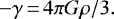
where x stands for kr, and α and β are the shear and compressional wave velocities:
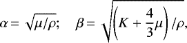 (B.29)
![Mathematical equation: \begin{equation*}k^2\,{=}\,\frac{1}{2}\left\{\frac{\omega^2+4\gamma}{\alpha^2}+\frac{\omega^2}{\beta^2}\,{\pm}\,\left[\left(\frac{\omega^2}{\beta^2}-\frac{\omega^2+4\gamma}{\alpha^2}\right){}^2+\frac{4l(l+1)\gamma^2}{\alpha^2\beta^2}\right]^{1/2}\right\},\end{equation*}](/articles/aa/full_html/2021/06/aa39433-20/aa39433-20-eq60.png) (B.30)
(B.30)
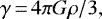 (B.31)
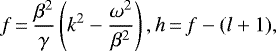 (B.32)
![Mathematical equation: \begin{equation*}\begin{array}{ll}{\hspace*{-6pt}}\Phi_l(x)& =\frac{(2l+1)!!}{x^l}j_l(x)\\[5pt]&=1-\frac{x^2}{2(2l+3)\,{\times}\,1}+\frac{x^4}{2^2(2l+3)(2l+5)\,{\times}\,2}- ...\!\!\end{array},\end{equation*}](/articles/aa/full_html/2021/06/aa39433-20/aa39433-20-eq63.png) (B.33)
(B.33)
![Mathematical equation: \begin{equation*}\Psi_l(x)\,{=}\,\frac{2(2l+3}{x^2}\left[1-\Phi_l(x)\right].\end{equation*}](/articles/aa/full_html/2021/06/aa39433-20/aa39433-20-eq64.png) (B.34)
(B.34)
For a liquid core (μ = 0), one of these two solutions disappears and we have
![Mathematical equation: \begin{equation*}\begin{array}{lll}{\hspace*{-6pt}} k^2&=&\left[\omega^2+4\gamma- \frac{l(l+1)\gamma^2}{\omega^2}\right]/\alpha^2\\[5pt]{\hspace*{-6pt}} f&=&-\omega^2/\gamma, h\,{=}\,f-(l+1) \!\!\end{array}.\end{equation*}](/articles/aa/full_html/2021/06/aa39433-20/aa39433-20-eq65.png) (B.35)
(B.35)
Continuation of solutions at liquid-solid interface
As explained in Appendix B.2, only two independent solutions exists in a liquid–fluid layer (μ = 0), while in a solid layer there are three solutions. This requires the redefinition of the third solution at a liquid–solid interface. The continuity conditions impose that
 (B.36)
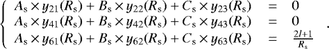
Boundary conditions at the surface
At the surface the stress must vanish to zero, so that y2 (Rs) = 0 and y4 (Rs) = 0. The potential should satisfy continuity across the boundary, so that 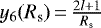 . For a solid surface the constants As, Bs, and Cs can be determined from the imposed boundary conditions:
 (B.37)
For a liquid–fluid surface these relationships reduce to
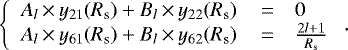 (B.38)
This particular case does not apply to the present study, where the surface is solid, but it can be useful for planets with an extended fluid envelop, such as lava worlds, Venus-like planets, or ocean-planets.
Numerical integration and reconstruction of the yi radial functions
Using for the first integration step the initial values computed from Eqs. (B.23)–(B.35) derived for a homogeneous sphere, the system of six differential equations (Eqs. (B.11)–(B.16)) for a solid layer; Eqs. (B.17)–(B.21) for a liquid layer) are solved by integrating the three or two independent solutions (depending on whether the considered layer is solid or liquid), using a fifth-order Runge-Kutta method with adaptive step-size control from the center (r = dr) to the surface (r = Rs), and by applying the appropriate continuity conditions (Eq. (B.37)) each time a liquid–solid interface is encountered.
The constants ((As, Bs, and Cs) or (Al and Bl)) are finally determined at the surface from the imposed surface conditions (using Eqs. (B.37) or (B.38), depending on whether the surface is solid or liquid). Using these constants, the full solution of the radial functions yi is then constructed from the three independent yij solutions. Particular attention must be paid each time a solid–liquid or liquid–solid interface is met. At the first solid–liquid interface, onthe solid side we have
 (B.39)
and on the liquid side
 (B.40)
with Al = As and Bl = Bs. At the base of the liquid layer, the Cs must be redefined in order to satisfy the continuity condition such that
 (B.41)
At each liquid–solid interface this procedure must be applied in order to correctly determine the entire yi profiles.
Although the whole set of equations described above have been initially derived for the elastic case, they can be used for the viscoleastic case by invoking the correspondence principle (Biot 1954) and defining the corresponding complex moduli,  and
and  (Eqs. (9) and (10)) and redefining all variables of the problem as complex variables (see Tobie et al. 2005, for more details).
Appendix C Radial sensitivity functions to shear and bulk moduli
Below we provide the expression of the radial sensitivity functions Hμ and HK used to compute the radial distribution of the tidal dissipation rate (Eq. (12)), taking into account both shear and bulk dissipation processes. The full derivation of these sensitivity functions from variational equations can be found in Tobie et al. (2005) and is not repeated here:
![Mathematical equation: \begin{eqnarray*}\begin{array}{ll}{\hspace*{-6pt}} H_{\textrm{K}} = &\frac{r^{2}}{|\tilde{K}+4/3\tilde{\mu}|^{2}}\left|y_2-\frac{\tilde{K}-2/3\tilde{\mu}}{r}[2y_1-l(l+1)y_3]\right|^2\\[5pt]&+2r \Re\left\{\frac{\textrm{d}y_1^{*}}{\textrm{d}r}[2y_1-l(l+1)y_3]\right\}\\[5pt]&+\left|2y_1-l(l+1)y_3\right|^2,\end{array} \nonumber \\[-15pt]\end{eqnarray*}](/articles/aa/full_html/2021/06/aa39433-20/aa39433-20-eq75.png) (C.1)
(C.1)
![Mathematical equation: \begin{equation*}\begin{array}{ll}{\hspace*{-6pt}} H_{\mu} = &\frac{4}{3}\frac{r^{2}}{|\tilde{K}+4/3\tilde{\mu}|^{2}}\left|y_2-\frac{\tilde{K}-2/3\tilde{\mu}}{r}[2y_1-l(l+1)y_3]\right|^2\\[5pt]& -\frac{4}{3}r\Re\left\{\frac{\textrm{d}y_1^{*}}{\textrm{d}r}[2y_1-l(l+1)y_3]\right\}+\frac{1}{3}\left|2y_1-l(l+1)y_3\right|^2\\[5pt]& +l(l+1)r^2|y_4|^2/|\mu|^2+l(l^2-1)(l+2)|y_3|^2.\\\end{array}\end{equation*}](/articles/aa/full_html/2021/06/aa39433-20/aa39433-20-eq76.png) (C.2)
(C.2)
The asterisk (*) stands for the complex conjugate, ℜ for the real part of a complex quantity, and |∙| corresponds to the modulus of ∙.
Appendix D Stress and strain tensors
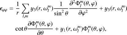
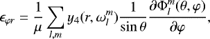
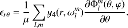
The complex strain and stress tensors, which are used in Eq. (13) to derive the local dissipation rate, are computed from the six radial complex functions yi (see Appendix B) at each grid point of the satellite interior. In spherical geometry the strain tensor components associated with the displacement field are
 (D.1)
(D.1)
 (D.2)
(D.2)
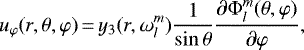
![Mathematical equation: \begin{equation*}\epsilon_{\theta \varphi} = \frac{2}{r} \sum_{l,m} y_3 (r, \omega_l^m) \frac{1}{\sin \theta} \Bigg[\frac{\partial^2 \Phi_l^m (\theta, \varphi)}{\partial \varphi \partial \theta} - \cot \theta \frac{\partial \Phi_l^m (\theta, \varphi)}{\partial \varphi} \Bigg],\end{equation*}](/articles/aa/full_html/2021/06/aa39433-20/aa39433-20-eq79.png) (D.3)
(D.3)
 (D.4)
(D.4)
 (D.5)
(D.5)
 (D.6)
(D.6)
We note that two components of the tidal strain tensor (ϵθφ and ϵφφ) were misprinted in Tobie et al. (2005) (Eq. (10)).
The corresponding stress tensor components are
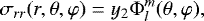 (D.7)
(D.7)
![Mathematical equation: \begin{eqnarray*}&& {\hspace*{-6pt}} \sigma_{\theta\theta}(r,\theta,\varphi) = \left\{(K-\frac{2}{3}\mu)\frac{\textrm{d}y_{1}}{\textrm{d}r}+\frac{K+\frac{4}{3}\mu}{r}[2y_{1}-l(l+1)y_{3}]-\frac{2\mu}{r}y_{1}\right\} \nonumber \\&& {\hspace*{-6pt}} \Phi_{l}^{m}(\theta,\varphi) -\frac{2\mu}{r}y_{3}\left(\frac{\cos\theta}{\sin\theta}\frac{\partial\Phi_{l}^{m}}{\partial \theta}+\frac{1}{\sin^{2}\theta}\frac{\partial^{2}\partial\Phi_{l}^{m}}{\partial\varphi^{2}}\right),\end{eqnarray*}](/articles/aa/full_html/2021/06/aa39433-20/aa39433-20-eq84.png) (D.8)
(D.8)
![Mathematical equation: \begin{eqnarray*}&& {\hspace*{-6pt}} \sigma_{\varphi\varphi}(r,\theta,\varphi) = \left\{(K-\frac{2}{3}\mu)\frac{\textrm{d}y_{1}}{\textrm{d}r}+\frac{K+\frac{4}{3}\mu}{r}[2y_{1}-l(l+1)y_{3}]-\frac{2\mu}{r}y_{1}\right\} \nonumber \\&& {\hspace*{-6pt}} \Phi_{l}^{m}(\theta,\varphi)-\frac{2\mu}{r}y_{3}\frac{\partial\Phi_{l}^{m}}{\partial\theta^{2}},\end{eqnarray*}](/articles/aa/full_html/2021/06/aa39433-20/aa39433-20-eq85.png) (D.9)
(D.9)
 (D.10)
 (D.11)
 (D.12)
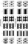 |
Fig. D.1 Patterns of stress and strain components. |
References
- Alterman, Z., Jarosch, H., & Pekeris, C. L. 1959, Proc. R. Soc. London Ser. A, 252, 80 [Google Scholar]
- Anderson, D. L. 1980, Nature, 285, 204 [Google Scholar]
- Anderson, D. L., & Sammis, C. 1970, Phys. Earth Planet. Int., 3, 41 [Google Scholar]
- Anderson, J., Sjogren, W., & Schubert, G. 1996, Science, 272, 709 [Google Scholar]
- Anderson, J. D., Jacobson, R. A., Lau, E. L., Moore, W. B., & Schubert, G. 2001, J. Geophys. Res. Planets, 106, 32963 [Google Scholar]
- Arzi, A. A. 1978, Tectonophysics, 44, 173 [Google Scholar]
- Bagdassarov, N., & Dingwell, D. B. 1993, J. Geophys. Res. Solid Earth, 98, 6477 [Google Scholar]
- Barnes, R., Raymond, S. N., Greenberg, R., Jackson, B., & Kaib, N. A. 2010, ApJ, 709, L95 [Google Scholar]
- Barr, A. C., Dobos, V., & Kiss, L. L. 2018, A&A, 613, A37 [NASA ADS] [CrossRef] [EDP Sciences] [Google Scholar]
- Běhounková, M., Tobie, G., Choblet, G., & Čadek, O. 2011, ApJ, 728, 89 [Google Scholar]
- Berckhemer, H., Kampfmann, W., Aulbach, E., & Schmeling, H. 1982, Phys. Earth Planet. Int., 29, 30 [Google Scholar]
- Beuthe, M. 2013, Icarus, 223, 308 [Google Scholar]
- Beuthe, M. 2019, Icarus, 332, 66 [Google Scholar]
- Bierson, C., & Nimmo, F. 2016, J. Geophys. Res. Planets, 121, 2211 [Google Scholar]
- Biot, M. A. 1954, J. Appl. Phys., 25, 1385 [Google Scholar]
- Blöcker, A., Saur, J., Roth, L., & Strobel, D. F. 2018, J. Geophys. Res. Space Phys., 123, 9286 [Google Scholar]
- Bonati, I., Lichtenberg, T., Bower, D. J., Timpe, M. L., & Quanz, S. P. 2019, A&A, 621, A125 [CrossRef] [EDP Sciences] [Google Scholar]
- Budiansky, B., & O’Connell, R. J. 1976, Int. J. Solids Struc., 12, 81 [Google Scholar]
- Budiansky, B., Sumner Jr, E. E., & O’Connell, R. J. 1983, J. Geophys. Rese. Solid Earth, 88, 10343 [Google Scholar]
- Buland, R., Berger, J., & Gilbert, F. 1979, Nature, 277, 358 [Google Scholar]
- Bulau, J., Waff, H., & Tyburczy, J. 1979, J. Geophys. Res. Solid Earth, 84, 6102 [Google Scholar]
- Caricchi, L., Burlini, L., Ulmer, P., et al. 2007, Earth Planet. Sci. Lett., 264, 402 [Google Scholar]
- Carr, M. H. 1986, J. Geophys. Res. Solid Earth, 91, 3521 [Google Scholar]
- Carr, M. H., McEwen, A. S., Howard, K. A., et al. 1998, Icarus, 135, 146 [Google Scholar]
- Castillo-Rogez, J. C., Efroimsky, M., & Lainey, V. 2011, J. Geophys. Res. Planets, 116, E09008 [Google Scholar]
- Christensen, N. I. 1996, J. Geophys. Res. Solid Earth, 101, 3139 [Google Scholar]
- Cooper, R., & Kohlstedt, D. 1986, J. Geophys. Res. Solid Earth, 91, 9315 [Google Scholar]
- Cooper, R., Kohlstedt, D., & Chyung, K. 1989, Acta Metallurgica, 37, 1759 [Google Scholar]
- Costa, A., Caricchi, L., & Bagdassarov, N. 2009, Geochem. Geophys. Geosyst. 10, 3 [Google Scholar]
- Davies, A. G., Veeder, G. J., Matson, D. L., & Johnson, T. V. 2015, Icarus, 262, 67 [Google Scholar]
- Dratler, J., Farrell, W., Block, B., & Gilbert, F. 1971, Geophys. J. Int., 23, 399 [Google Scholar]
- Durek, J. J., & Ekström, G. 1995, Geophys. Res. Lett., 22, 2309 [Google Scholar]
- Dziewonski, A. M., & Anderson, D. L. 1981, Phys. Earth Planet. Int., 25, 297 [Google Scholar]
- Efroimsky, M. 2012, ApJ, 746, 150 [Google Scholar]
- Faul, U. H., & Jackson, I. 2007, J. Geophys. Res. Solid Earth, 112, B4 [Google Scholar]
- Fischer, H.-J., & Spohn, T. 1990, Icarus, 83, 39 [Google Scholar]
- Hamilton, C. W., Beggan, C. D., Still, S., et al. 2013, Earth Planet. Sci. Lett., 361, 272 [Google Scholar]
- Heinz, D., Jeanloz, R., & O’Connell, R. J. 1982, J. Geophys. Res. Solid Earth, 87, 7772 [Google Scholar]
- Henning, W. G., Renaud, J. P., Saxena, P., et al. 2018, ArXiv e-prints [arXiv:1804.05110] [Google Scholar]
- Hirth, G., & Kohlstedt, D. L. 1995a, J. Geophys. Res. Solid Earth, 100, 15441 [Google Scholar]
- Hirth, G., & Kohlstedt, D. L. 1995b, J. Geophys. Res. Solid Earth, 100, 1981 [Google Scholar]
- Holmes, M., Parker, N., & Povey, M. 2016 2011, IOP Publishing, 012011 [Google Scholar]
- Holtzman, B. K. 2016, Geochem. Geophys. Geosys., 17, 470 [Google Scholar]
- Jackson, I. 1998, Geophys. J. Int., 134, 291 [Google Scholar]
- Jackson, J. M., Zhang, J., & Bass, J. D. 2004, Geophys. Res. Lett., 31, L15608 [Google Scholar]
- Jaupart, C., Labrosse, S., & Mareschal, J. 2007, Treatise Geophys., 7, 223 [Google Scholar]
- Ji, S., Li, L., Motra, H. B., et al. 2018, J. Geophys. Res. Solid Earth, 123, 1161 [Google Scholar]
- Karato, S.-i. 2012, Earth Planet. Sci. Lett., 321, 95 [Google Scholar]
- Karato, S.-i., & Wu, P. 1993, Science, 260, 771 [Google Scholar]
- Keszthelyi, L., Jaeger, W., Milazzo, M., et al. 2007, Icarus, 192, 491 [Google Scholar]
- Khurana, K. K., Jia, X., Kivelson, M. G., et al. 2011, Science, 332, 1186 [Google Scholar]
- Kirchoff, M. R., McKinnon, W. B., & Schenk, P. M. 2011, Earth Planet. Sci. Lett., 301, 22 [Google Scholar]
- Kohlstedt, D. L., & Zimmerman, M. E. 1996, Annu. Rev. Earth Planet. Sci., 24, 41 [Google Scholar]
- Kohlstedt, D. L., Bai, Q., Wang, Z.-C., & Mei, S. 2000, in Physics and Chemistry of Partially Molten Rocks (Berlin: Springer), 3 [Google Scholar]
- Labrosse, S., Hernlund, J., & Coltice, N. 2007, Nature, 450, 866 [Google Scholar]
- Lainey, V., Arlot, J.-E., Karatekin, Ö., & Van Hoolst, T. 2009, Nature, 459, 957 [Google Scholar]
- Lejeune, A.-M., & Richet, P. 1995, J. Geophys. Res. Solid Earth, 100, 4215 [Google Scholar]
- Mavko, G. M. 1980, J. Geophys. Res. Solid Earth, 85, 5173 [Google Scholar]
- McEwen, A. S., Keszthelyi, L., Spencer, J., et al. 1998, Science, 281, 87 [Google Scholar]
- McEwen, A. S., Belton, M., Breneman, H., et al. 2000, Science, 288, 1193 [Google Scholar]
- McKenzie, D. 1984, J. Petrol., 25, 713 [Google Scholar]
- Mei, S., Bai, W., Hiraga, T., & Kohlstedt, D. L. 2002, Earth Planet. Sci. Lett., 201, 491 [Google Scholar]
- Monnereau, M., & Dubuffet, F. 2002, Icarus, 158, 450 [Google Scholar]
- Moore, W. 2003, J. Geophys. Res. Planets, 108, E12 [Google Scholar]
- Moore, W. B. 2001, Icarus, 154, 548 [Google Scholar]
- Morozov, I. B. 2015, Bull. Seismol. Soc. Am., 105, 3180 [Google Scholar]
- Murase, T., & McBirney, A. R. 1973, Geolog. Soc. Am. Bull., 84, 3563 [Google Scholar]
- O’Connell, R. J., & Budiansky, B. 1977, J. Geophys. Res., 82, 5719 [Google Scholar]
- Peale, S. J., Cassen, P., & Reynolds, R. T. 1979, Science, 203, 892 [Google Scholar]
- Pekeris, C., & Jarosh, H. 1958, The Free Oscillations of the Earth, Contributions in Geophysics (Gutenberg Volume) (Amsterdam: Elsevier), 171 [Google Scholar]
- Peltier, W. 1974, Rev. Geophysi., 12, 649 [Google Scholar]
- Renaud, J. P., & Henning, W. G. 2018, ApJ, 857, 98 [Google Scholar]
- Renner, J., Evans, B., & Hirth, G. 2000, Earth Planet. Sci. Lett., 181, 585 [Google Scholar]
- Renner, J., Viskupic, K., Hirth, G., & Evans, B. 2003, Geochem. Geophys. Geosyst. 4, 8606 [Google Scholar]
- Ricard, Y., Bercovici, D., & Schubert, G. 2001, J. Geophys. Res. Solid Earth, 106, 8907 [Google Scholar]
- Rivers, M. L., & Carmichael, I. S. 1987, J. Geophys. Res. Solid Earth, 92, 9247 [Google Scholar]
- Romanowicz, B., & Mitchell, B. 2007, Treatise Geophys., 731 [Google Scholar]
- Roscoe, R. 1952, British J. Appl. Phys., 3, 267 [Google Scholar]
- Ross, M., Schubert, G., Spohn, T., & Gaskell, R. 1990, Icarus, 85, 309 [Google Scholar]
- Roth, L., Saur, J., Retherford, K. D., et al. 2017, J. Geophys. Res. Space Phys., 122, 1903 [Google Scholar]
- Rudge, J. F. 2018, J. Geophys. Res. Solid Earth, 123, 10 [Google Scholar]
- Sailor, R. V., & Dziewonski, A. M. 1978, Geophys. J. Int., 53, 559 [Google Scholar]
- Saito, M. 1974, J. Phys. Earth, 22, 123 [Google Scholar]
- Schenk, P., Hargitai, H., Wilson, R., McEwen, A., & Thomas, P. 2001, J. Geophys. Res. Planets, 106, 33201 [Google Scholar]
- Schmeling, H. 1985, Phys. Earth Planet. Int., 41, 34 [Google Scholar]
- Schmeling, H., Kruse, J. P., & Richard, G. 2012, Geophys. J. Int., 190, 1571 [Google Scholar]
- Scott, T., & Kohlstedt, D. L. 2006, Earth Planet. Sci. Lett., 246, 177 [Google Scholar]
- Scott, D. R., & Stevenson, D. J. 1986, J. Geophys. Res. Solid Earth, 91, 9283 [Google Scholar]
- Segatz, M., Spohn, T., Ross, M., & Schubert, G. 1988, Icarus, 75, 187 [Google Scholar]
- Shaw, H., Wright, T., Peck, D., & Okamura, R. 1968, Am. J. Sci., 266, 225 [Google Scholar]
- Simpson, G., Spiegelman, M., & Weinstein, M. I. 2010, J. Geophys. Rese. Solid Earth, 115, B4 [Google Scholar]
- Sohl, F., Spohn, T., Breuer, D., & Nagel, K. 2002, Icarus, 157, 104 [Google Scholar]
- Spencer, J. R., Jessup, K. L., McGrath, M. A., Ballester, G. E., & Yelle, R. 2000, Science, 288, 1208 [Google Scholar]
- Spencer, D. C., Katz, R. F., & Hewitt, I. J. 2020, J. Geophys. Res. Planets, 125, e06443 [Google Scholar]
- Spohn, T. 1997, in Tidal Phenomena (Berlin: Springer), 345 [Google Scholar]
- Steinke, T., Hu, H., Höning, D., van der Wal, W., & Vermeersen, B. 2020, Icarus, 335, 113299 [Google Scholar]
- Stolper, E., Walker, D., Hager, B. H., & Hays, J. F. 1981, J. Geophys. Res. Solid Earth, 86, 6261 [Google Scholar]
- Sundberg, M., & Cooper, R. F. 2010, Philos. Magazine, 90, 2817 [Google Scholar]
- Takei, Y. 1998, J. Geophys. Res. Solid Earth, 103, 18183 [Google Scholar]
- Takei, Y., & Holtzman, B. K. 2009, J. Geophys. Res. Solid Earth, 114, B6 [Google Scholar]
- Takeuchi, H., & Saito, M. 1972, Methods Comput. Phys., 11, 217 [Google Scholar]
- Tobie, G., Mocquet, A., & Sotin, C. 2005, Icarus, 177, 534 [Google Scholar]
- Tobie, G., Grasset, O., Dumoulin, C., & Mocquet, A. 2019, A&AS, 630, A70 [Google Scholar]
- Turbet, M., Bolmont, E., Leconte, J., et al. 2018, A&A, 612, A86 [CrossRef] [EDP Sciences] [Google Scholar]
- Tyler, R. H., Henning, W. G., & Hamilton, C. W. 2015, ApJS, 218, 22 [Google Scholar]
- Usselman, T. M. 1975, Am. J. Sci., 275, 278 [Google Scholar]
- Van der Molen, I., & Paterson, M. 1979, Contrib. Mineral. Petrol., 70, 299 [Google Scholar]
- Veeder, G. J., Matson, D. L., Johnson, T. V., Blaney, D. L., & Goguen, J. D. 1994, J. Geophys. Res. Planets, 99, 17095 [Google Scholar]
- Veeder, G. J., Davies, A. G., Matson, D. L., et al. 2012, Icarus, 219, 701 [Google Scholar]
- Vigneresse, J. L., Barbey, P., & Cuney, M. 1996, J. Petrol., 37, 1579 [Google Scholar]
- Walsh, J. 1968, J. Geophys. Res., 73, 2209 [Google Scholar]
- Walsh, J. 1969, J. Geophys. Res., 74, 4333 [Google Scholar]
- Widmer, R., Masters, G., & Gilbert, F. 1991, Geophys. J. Int., 104, 541 [Google Scholar]
- Wisdom, J. 2008, Icarus, 193, 637 [Google Scholar]
All Tables
Density, rheological solid-state parameters, and interior structure characteristics assumed for Io’s interior.
All Figures
|
Fig. 1 Model of Io’s internal structure used for the computations. The considered rheology can be divided into three groups: (1) the solid mantle and crust, described by an Andrade rheology neglecting bulk dissipation; (2) the partially molten layers, either beneath the crust (case A) or at the core mantle boundary (case B), or a combination of both (Case C), described by a Maxwell rheology including both shear and bulk dissipation and accounting for the effect of melt on the viscoelastic parameters (following the rheological law described in Sect. 3.2); (3) the inviscid liquid metallic core. |
| In the text | |
|
Fig. 2 Effect of melt fraction ϕ on the viscoelastic parameters: shear viscosity η and modulusμ (solid lines), bulk viscosity ζ and modulusK (dash-dotted lines). The red vertical dashed line denotes the rheological critical melt fraction (ϕc) where the transition between solid-state and liquid-state behaviors occurs. The shaded rectangle illustrates the restriction of our investigation to a range of melt fraction values around the RCMF. |
| In the text | |
|
Fig. 3 Io’s tidal heat budget as a function of melt fraction ϕ and the thickness dmelt of the partially molten layer(s). Three configurations are considered for the internal structure (see Fig. 1): with one partially molten layer at the top (case A, left column) or at the bottom of the mantle (case B, middle column), or with partially molten layers both at the top and bottom of the mantle (case C, right column). The color scale refers to the global tidal power Pbulk, including the contribution of bulk dissipation (top panel), and to the ratio (Pbulk − Pnobulk)∕Pnobulk, with Pnobulk designating the reference global tidal power produced with shear dissipation only (bottom panel). The red curves highlight the 100 TW value. The black curve indicates the parameters required to obtain this same value without bulk dissipation. For each configuration the red star denotes a reference case corresponding to a thickness dmelt = 100 km. The white dashed line indicates the value of ϕc. |
| In the text | |
|
Fig. 4 Io’s tidal heat budget Pglob as a function of melt fraction of the partially molten layer. Configurations for the interior structure involve: a top partially molten layer (case A, red), a bottom partially molten layer (case B, green), and a combination of the two, both layers being of equal thickness (case C, blue). The layers thickness is dmelt = 100 km. Cases involving bulk dissipation correspond to solid curves. Cases where bulk dissipation is not included correspond to dash-dotted curves. The shaded rectangle gives Io’s heat budget range (65–125 TW; see, e.g., Lainey et al. 2009). |
| In the text | |
|
Fig. 5 Radial distribution of the tidal dissipation rate |
| In the text | |
|
Fig. 6 Patterns of tidal heat flux qtide integrated over the top partially molten layer for one orbit cycle at a given location for the reference model denoted by a red star in Fig. 3, Case A, corresponding to ϕ = 0.3122. Left: values obtained when bulk dissipation is accounted for (providing a total power Pbulk = 100 TW). Right:values obtained when bulk dissipation is not accounted for; in this case the total power is less than 100 TW (45 TW). The same scale is used to highlight the tidal power enhancement due to bulk dissipation. |
| In the text | |
|
Fig. 7 Patterns of tidal heat flux qtide integratedover the bottom partially molten layer for one orbit cycle at a given location for the reference model denoted by a red star in Fig. 3, Case B, corresponding to ϕ = 0.3106. Left: values obtained when bulk dissipation is accounted for (providing a total power Pbulk = 100 TW). Right:values obtained when bulk dissipation is not accounted for; in this case the total power is less than 100 TW (12 TW). The two color scales are not the same. |
| In the text | |
|
Fig. D.1 Patterns of stress and strain components. |
| In the text | |
Current usage metrics show cumulative count of Article Views (full-text article views including HTML views, PDF and ePub downloads, according to the available data) and Abstracts Views on Vision4Press platform.
Data correspond to usage on the plateform after 2015. The current usage metrics is available 48-96 hours after online publication and is updated daily on week days.
Initial download of the metrics may take a while.