| Issue |
A&A
Volume 582, October 2015
|
|
|---|---|---|
| Article Number | A115 | |
| Number of page(s) | 10 | |
| Section | Cosmology (including clusters of galaxies) | |
| DOI | https://doi.org/10.1051/0004-6361/201526461 | |
| Published online | 21 October 2015 | |
New measurements of Ωm from gamma-ray bursts
1
Dip. di Fisica, Sapienza Universitá di Roma,
Piazzale Aldo Moro 5,
00185
Rome,
Italy
2
ICRANet-Pescara, Piazza della Repubblica 10,
65122
Pescara,
Italy
e-mail: This email address is being protected from spambots. You need JavaScript enabled to view it.
; This email address is being protected from spambots. You need JavaScript enabled to view it.
3
ICRANet-Rio, Centro Brasileiro de Pesquisas Fisicas, Rua Dr.
Xavier Sigaud 150, 22290-180
Rio de Janeiro,
Brazil
e-mail: This email address is being protected from spambots. You need JavaScript enabled to view it.
4
INAF–Istituto di Astrofisica Spaziale e Fisica Cosmica, Bologna,
via Gobetti 101, 40129
Bologna,
Italy
5
INAF–Napoli, Osservatorio Astronomico di Capodimonte, Salita
Moiariello 16, 80131
Napoli,
Italy
Received:
4
May
2015
Accepted:
24
August
2015
Abstract
Context. Data from cosmic microwave background radiation (CMB), baryon acoustic oscillations (BAO), and supernovae Ia (SNe-Ia) support a constant dark energy equation of state with w0 ~ −1. Measuring the evolution of w along the redshift is one of the most demanding challenges for observational cosmology.
Aims. We discuss the existence of a close relation for gamma-ray bursts (GRBs), named Combo-relation, based on characteristic parameters of GRB phenomenology such as the prompt intrinsic peak energy Ep,i, the X-ray afterglow initial luminosity L0 and the rest-frame duration τ of the shallow phase, and the index of the late power-law decay αX. We use it to measure Ωm and the evolution of the dark energy equation of state. We also propose a new calibration method for the same relation, which reduces the dependence on SNe Ia systematics.
Methods. We have selected a sample of GRBs with 1) a measured redshift z; 2) a determined intrinsic prompt peak energy Ep,i; and 3) a good coverage of the observed (0.3–10) keV afterglow light curves. The fitting technique of the rest-frame (0.3–10) keV luminosity light curves represents the core of the Combo-relation. We separate the early steep decay, considered a part of the prompt emission, from the X-ray afterglow additional component. Data with the largest positive residual, identified as flares, are automatically eliminated until the p-value of the fit becomes greater than 0.3.
Results. We strongly minimize the dependency of the Combo-GRB calibration on SNe Ia. We also measure a small extra-Poissonian scatter of the Combo-relation, which allows us to infer from GRBs alone ΩM = 0.29+0.23-0.15 (1σ) for the ΛCDM cosmological model, and ΩM = 0.40+0.22-0.16, w0 = −1.43+0.78-0.66 for the flat-Universe variable equation of state case.
Conclusions. In view of the increasing size of the GRB database, thanks to future missions, the Combo-relation is a promising tool for measuring Ωm with an accuracy comparable to that exhibited by SNe Ia, and to investigate the dark energy contribution and evolution up to z ~ 10.
Key words: cosmological parameters / gamma-ray burst: general / dark energy
© ESO, 2015
1. Introduction
Gamma-ray bursts (GRBs) are observed in a wide range of spectroscopic and photometric redshifts, up to z ~ 9 (Salvaterra et al. 2009; Tanvir et al. 2009; Cucchiara et al. 2011). This suggests that GRBs can be used to probe the high-z Universe, in terms of investigating the re-ionization era, population III stars, the metallicity of the circumburst medium, the faint-end of galaxies luminosity evolution (D’Elia et al. 2007; Robertson & Ellis 2012; Macpherson et al. 2013; Trenti et al. 2013, 2015), and as cosmological rulers (e.g. Ghirlanda et al. 2004; Dai et al. 2004; Amati & Della Valle 2013). The latter works show that GRBs, through the correlation between radiated energy or luminosity and the photon energy at which their νF(ν) spectrum peaks Ep,i, admittedly with a lower level of accuracy, provide results in agreement with supernovae Ia (SN Ia, Perlmutter et al. 1998, 1999; Schmidt et al. 1998; Riess et al. 1998), baryonic acoustic oscillations (BAO, Blake et al. 2011), and cosmic microwave background (CMB) radiation (Planck Collaboration XVI 2014). The Universe is spatially flat (e.g. de Bernardis et al. 2000), and it is dominated by a still unknown vacuum energy, usually called dark energy, which is responsible for the observed acceleration. Measuring the equation of state (EOS, ω = p/ρ, with p the pressure and ρ the density of the dark energy) is one of the most difficult tasks in observational cosmology today. Current data (Suzuki et al. 2012; Planck Collaboration XIII 2015) suggest that w0 ~ −1 and wa ~ 0, the expected values for the cosmological constant. Although these results are probably sufficient to exclude a very rapid evolution of dark energy with z, we cannot yet exclude that it may evolve with time, as originally proposed by Bronstein (1933). In principle, with SNe Ia we can push our investigation up to z ≈ 1.7 (Suzuki et al. 2012). However we note that the possibility of detecting SNe Ia at higher redshifts will depend on the availability of next-generation telescopes and also on the time delay distribution of SNe Ia (see Fig. 8 in Mannucci et al. 2006).
A solution to this problem may be provided by GRBs: their redshift distribution peaks around z ~ 2−2.5 (Coward et al. 2013) and extends up to the photometric redshift of z = 9.4, (Cucchiara et al. 2011). Therefore, given this broad range of z and their very high luminosities, GRBs are a class of objects suitable to explore the trend of dark energy density with time (Lloyd & Petrosian 1999; Ramirez-Ruiz & Fenimore 2000; Reichart et al. 2001; Norris et al. 2000; Amati et al. 2002, 2008; Ghirlanda et al. 2004; Dai et al. 2004; Yonetoku et al. 2004; Firmani et al. 2006; Liang & Zhang 2006; Schaefer 2007; Capozziello & Izzo 2008; Dainotti et al. 2008; Tsutsui et al. 2009; Wei et al. 2014; Wang et al. 2015). There are two complications connected with these approaches. First, the correlations are always calibrated by using the entire range of SNe Ia up to z = 1.7; therefore, this procedure strongly biases the GRB cosmology and for our purposes we need the highest level of independent calibration possible. Second, the data scatter of these correlations is not tight enough to constrain cosmological parameters (in this work we refer to the different extra-scatters published in Margutti et al. 2013), even when a large GRB dataset is used. In this work we present a method that can override the latter and minimize the former.
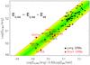 |
Fig. 1 EX,iso–Eγ,iso–Ep,i correlation proposed by Bernardini et al. (2012) and Margutti et al. (2013) (courtesy R. Margutti). |
Very recently Bernardini et al. (2012, hereafter B12) and Margutti et al. (2013, hereafter M13) have published an interesting correlation that connects the prompt and the afterglow emission of GRBs (see Fig. 1). This relation strongly links the X-ray and γ-ray isotropic energy with the intrinsic peak energy, 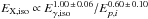 , unveiling an interesting connection between the early, more energetic component of GRBs (Eγ,iso and Ep,i) and their late emission (EX,iso), opportunely filtered for flaring activity. In addition, the intrinsic extra scatter is very small σEX,iso = 0.30 ± 0.06 (1σ). Starting from the results obtained by B12 and M13, and combining them with the well-known Ep,i − Eiso relation (Amati et al. 2002), we present here a new correlation involving four GRB parameters, which we named the Combo-relation. This new relation is then used to measure Ωm and to explore the possible evolution of w of EOS with the redshift by using as a “candle” the initial luminosity L0 of the shallow phase of the afterglow, which we find to be strictly correlated with quantities directly inferred from observations.
The paper is organized as follows. In Sect. 2 we describe in detail how we obtain the formulation of the newly proposed GRB correlation, and present the sample of GRBs used to test our results, the procedure for the fitting of the X-ray afterglow light curves, and finally, the existence of the correlation assuming a standard cosmological scenario. Then, in Sect. 3, we discuss the use of the relation as cosmological parameter estimator, which involves a calibration technique that does not require the use of the entire sample of SNe Ia, as was often done in previous similar works. In Sect. 4, we test the use of GRBs estimating the main cosmological parameters, as well as the evolution of the dark energy EOS. Finally, we discuss the final results in the last section.
2. The Combo-relation
We present here a new GRB correlation, the Combo-relation, obtained after combining Eγ,iso–EX,iso–Ep,i (B12 and M13), the Eγ,iso–Ep,i (Amati et al. 2002) correlations, and the analytical formulation of the X-ray afterglow component given in Ruffini et al. (2014, hereafter R14).
The three-parameter scaling law reported in B12 and M13 can be generally written as  (1)where EX,iso is the isotropic energy of a GRB afterglow in the rest-frame (0.3–30) keV energy range obtained by integrating the light curve in luminosity over a specified time interval, Eγ,iso is the isotropic energy of a GRB prompt emission, and Ep,i is the intrinsic spectral peak energy of a GRB. Since EX,iso and Eγ,iso are both cosmological-dependent quantities, we reformulate this correlation in order to involve only one cosmological-dependent quantity.
The right term of Eq. (1) can be rewritten using the well-known formulation of the Amati relation,  , which provides
 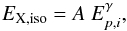 (2)where γ = η × β − δ and A is the normalization constant. Since the Amati relation is valid only for long bursts, in the following discussion we will exclude short GRBs with a rest-frame T90 duration smaller than 2 s, and short bursts with “extended emission” (Norris & Bonnell 2006), or “disguised short” GRBs (Bernardini et al. 2007; Caito et al. 2010), which have hybrid characteristic between short and long bursts.
To rewrite Eq. (2) for cosmological purposes, we have calculated the total isotropic X-ray energy in the rest-frame (0.3–10) keV energy range by integrating the X-ray luminosity  , expressed as a function of the cosmological rest-frame arrival time
  , over the time interval
  . This luminosity is obtained by considering four steps (see e.g. Appendix A and Pisani et al. 2013).
It is well known that the X-ray afterglow phenomenology can be described by the presence of an additional component emerging from the soft X-ray steep decay of the GRB prompt emission, and characterized by a first shallow emission, usually named the plateau, and a late power-law decay behaviour (Nousek et al. 2006; Zhang et al. 2006; Willingale et al. 2007). In addition, many GRB X-ray light curves are characterized by the presence of large, late-time flares, whose origin is very likely associated with late-time activity of the internal engine (Margutti et al. 2010). Since their luminosities are much lower than the prompt one, we exclude X-ray flares from our analysis via a light-curve fitting algorithm, which will be explained later in the text. We then make the assumption that the EX,iso quantity refers only to the component whose X-ray luminosity is given by the phenomenological function defined in R14  (3)where L0, τ, and αX are, respectively, the luminosity at
  , the characteristic timescale of the end of the shallow phase, and the late power-law decay index of a GRB afterglow.
Therefore, if we extend the integration time interval to  and
and  , the integral of the function in Eq. (3) gives
  (4)with the requirement that αX< −1. This condition is necessary to exclude divergent values of EX,iso computed from Eq. (4), for . It is worth noting that light curves providing values αX> −1 could have a change in slope at very late times (beyond the XRT time coverage) and/or, in principle, could be polluted by a late flaring activity, resulting in a less steep late decay.
Considering Eqs. (2) and (4), we can finally formulate the following relation between GRB observables  (5)which we name the Combo-relation. At first sight, Eq. (5) suggests the existence of a physical connection between specific physical properties of the afterglow and prompt emission in long GRBs. A two-dimensional fashion of the correlation in Eq. (5) in logarithmic units can be written as
 ![Mathematical equation: \begin{equation} \label{eq:no7} \log \left(\frac{L_0}{\textnormal{erg/s}}\right) = \log \left(\frac{A}{\textnormal{erg/s}}\right) + \gamma\left[ \log \left(\frac{E_{p,i}}{\textnormal{keV}}\right) - \frac{1}{\gamma}\log \left(\frac{\tau/\textnormal{s}}{|1+\alpha_{\rm X}|}\right)\right] , \end{equation}](/articles/aa/full_html/2015/10/aa26461-15/aa26461-15-eq59.png) (6)where the set of parameters in the square brackets has the meaning of a logarithmic independent coordinate, and in the following will be expressed as log [X(γ,Ep,i,τ,αX)].
(6)where the set of parameters in the square brackets has the meaning of a logarithmic independent coordinate, and in the following will be expressed as log [X(γ,Ep,i,τ,αX)].
We have tested the reliability of Eqs. (5) and (6) by building a sample of GRBs satisfying the following restrictions:
-
a measured redshift z;
-
a determined prompt emission spectral peak energy Ep,i;
-
a complete monitoring of the GRB X-ray afterglow light curve from the early decay (
 s, when present) until late emission (
 –106 s).
We start the analysis by computing the rest-frame (0.3–10) keV energy band light curves (see Appendix A). The fitting of the continuum part of the X-ray light curves was performed by using a semi-automated procedure based on the χ2 statistic, which eliminates the flaring part (see e.g. Appendix B and Margutti et al. 2011; Zaninoni 2013, and M13, for details). A total of 60 GRBs are found, whose distribution in the Combo-relation plane is shown in Fig. 2, where the value of the luminosity L0 for each GRB is calculated from the flat ΛCDM scenario. The corresponding best-fit parameters, as well as the extra-scatter term σext, have been derived by following the procedure by D’Agostini (2005), and are respectively log [A/ (erg / s)] = 49.94 ± 0.27, γ = 0.74 ± 0.10, and σext = 0.33 ± 0.04. The Spearman’s rank correlation coefficient is ρS = 0.92, while the p-value computed from the two-sided Student’s t-distribution, is pval = 9.13 × 10⁻²².
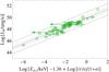 |
Fig. 2 Correlation considering the entire sample of 60 GRBs. The green empty boxes are the data of each of the sources, derived as described in Appendix B, the solid black line is the best fit of the data, while the dotted grey lines and the dashed grey lines correspond, respectively, to the dispersion on the correlation at 1σex and 3σex. |
3. Calibration of the Combo-relation
The lack of very nearby (z ~ 0.01) GRBs prevents the possibility of calibrating GRB correlations, as is usually done with SNe Ia. In recent years different methods have been proposed to avoid this “circularity problem” in calibrating GRB relations (Kodama et al. 2008; Demianski et al. 2012, and references therein). The common approach uses an interpolating function for the distribution of luminosity distances (distance moduli) of SNe Ia with redshift, and then extending it to GRBs at higher redshifts. In the following we introduce and describe an alternative method for calibrating the Combo-relation (see also Ghirlanda et al. 2006) which consists of two steps: 1) we identify a small but sufficient subsample of GRBs that lie at the same redshift, and then infer the slope parameter γ from a best-fit procedure; 2) once we determine γ, the luminosity parameter A can be obtained from a direct comparison between the nearest, z = 0.145, GRBs in our sample and SNe Ia located at very similar redshifts. We note that this approach is different from previous ones in that we do not use the whole redshift range covered by SNe Ia, but we limit our calibration analysis to z = 0.145 where the effect of the cosmology on the distance modulus of the calibrating SNe Ia is small (see Fig. 3).
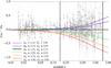 |
Fig. 3 Residual distance modulus μobs − μth for different values of the density cosmological parameters Ωm and ΩΛ up to z = 2.0. We consider the best fit to be the standard ΛCDM model, where Ωm = 0.27, ΩΛ = 0.73, and H0 = 71 km s-1/Mpc (black line). Union2 SNe Ia data residuals are shown in grey. The large spread (more than 1 mag) shown by μ at z = 1.5 and at z = 0.145 (the two vertical dashed lines) where the scatter is almost 0.2 mag is clearly evident. |
3.1. The determination of the slope γ
Five GRBs used for the determination of the slope parameter γ of the correlation.
The existence of a subsample with a sufficient number of GRBs lying at almost the same cosmological distance would, in principle, allow us to infer γ, overriding any possible cosmological dependence (assuming a homogeneous and isotropic Universe). In our sample of 60 GRBs there is a small subsample of 5 GRBs located at a very similar redshift, see Table 1. The difference between the maximum redshift of this 5-GRB sample (z = 0.544) and the minimum one (z = 0.5295) corresponds to a variation of 0.015 in redshift and of 0.07 in distance modulus μ in the case of the standard ΛCDM model. This very small difference is sufficient for our purposes.
To avoid any possible cosmological contamination, we do not consider the luminosity L0 as the dependent variable, but we consider instead the energy flux F0, which is related to the luminosity through the expression  . This assumption does not influence the final result, since dl is almost the same for the 5-GRB sample and, therefore, the
  term can be absorbed in the normalization constant. Consequently, we build the energy flux light curve for each GRB, and then, following the same procedure described in Sect. 2, we perform a best-fit analysis of this subsample of five GRBs using the maximum likelihood technique. From the best fit we find a value of γ = 0.89 ± 0.15, with an extra scatter of σext = 0.40 ± 0.04, see Fig. 4.
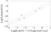 |
Fig. 4 Correlation found for the sample of five GRBs located at the same redshift. The blue triangles are the data of each of the five sources, derived from the procedure in Appendix B. The solid line represents the best fit while the dashed line is the dispersion on the correlation at 1σex. |
3.2. Calibration of A with SNe Ia
Among the considered 60 GRBs, the nearest one is GRB 130702A at z = 0.145. We use it to perform the calibration of the Combo-relation with SNe Ia located at the same distance. It is clear that at these redshifts (z = 0.145) the offset provided by SNe Ia is much smaller than the value inferred from SNe Ia at larger redshifts, see Fig. 3. In this light we have selected Union2 SNe Ia (Amanullah et al. 2010; Suzuki et al. 2012) with redshift between z = 0.143 and z = 0.147. We find five SNe Ia that satisfy this condition; their properties are shown in Table 2. We then compute the average value of their distance modulus and its uncertainty, ⟨ μ ⟩ = 39.19 ± 0.27, which will be used for the final calibration. The parameter A can be obtained inverting Eq. (6), and considering L0 = 4πdl2F0: 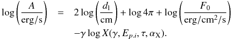 (7)The generic SN distance modulus μ can be directly related to the luminosity distance dl by
Five SNe Ia selected from the Union2 sample (Amanullah et al. 2010; Suzuki et al. 2012) and used for the calibration of the GRB correlation.
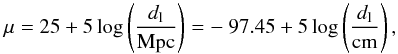 (8)where the last equality takes into account the fact that dl is expressed in cm. Substituting this last expression for
  in Eq. (7) we obtain
 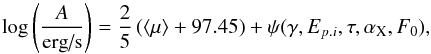 (9)where the term ψ(γ,Ep.i,τ,αX,F0) comprises the last three terms on the right hand side of Eq. (7). Substituting the quantities for GRB 130702A in Eq. (9), and the value of ⟨ μ ⟩ previously obtained, we infer a value for the parameter log [ A/ (erg / s) ] = 49.54 ± 0.20, where the uncertainty also takes the σext value found above into account.
4. Cosmology with the Combo-relation
4.1. Building the GRB Hubble diagram
We now discuss the possible use of the proposed GRB Combo-relation to measure the cosmological constant and the mass density, as well as their evolution with redshift z. The possibility of estimating the luminosity distance dl from the GRB observable quantities allows to us define a distance modulus for GRBs, and then its uncertainty, as ![Mathematical equation: \begin{equation} \label{eq:no11} \mu_{\rm GRB} = - 97.45 + \frac{5}{2} \left[\mathcal{A} - \psi(\gamma,E_{p,i},\tau,\alpha_{\rm X},F_0) \right], \end{equation}](/articles/aa/full_html/2015/10/aa26461-15/aa26461-15-eq139.png) (10)where
(10)where ![Mathematical equation: \hbox{$\mathcal{A}=\log [A/(\textnormal{erg/s})]$}](/articles/aa/full_html/2015/10/aa26461-15/aa26461-15-eq140.png) . The quantity μGRB can be directly compared with the theoretical cosmological expected value μth, which depends on the density parameters Ωm and ΩΛ, the curvature term Ωk = 1 − Ωm − ΩΛ, and the Hubble constant H0
. The quantity μGRB can be directly compared with the theoretical cosmological expected value μth, which depends on the density parameters Ωm and ΩΛ, the curvature term Ωk = 1 − Ωm − ΩΛ, and the Hubble constant H0 (11)The luminosity distance dl is defined as
 ![Mathematical equation: \begin{equation} \label{eq:no13} d_{\rm l} = \frac{c}{H_0}(1+z) \left\{ \begin{array}{lll} \frac{1}{\sqrt{| \Omega_k |}} \sinh \left[\int_0^z \frac{\sqrt{| \Omega_k |} {\rm d}z^\prime}{\sqrt{E(z^\prime,\,\Omega_{\rm m},\,\Omega_{\Lambda},\, w(z))}}\right] \hspace{-0.1cm},&\ \Omega_k > 0 \vspace{0.2cm}\\[2.5mm] \int_0^z \frac{{\rm d}z^\prime}{\sqrt{E(z^\prime,\,\Omega_{\rm m},\,\Omega_{\Lambda},\, w(z))}} \hspace{-0.1cm},&\ \Omega_k = 0 \vspace{0.2cm}\\[2.5mm] \frac{1}{\sqrt{| \Omega_k |}} \sin \left[ \int_0^z \frac{\sqrt{| \Omega_k |}{\rm d}z^\prime}{\sqrt{E(z^\prime,\,\Omega_{\rm m},\,\Omega_{\Lambda},\, w(z))}} \right] \hspace{-0.1cm},&\ \Omega_k < 0 \end{array} \right. \end{equation}](/articles/aa/full_html/2015/10/aa26461-15/aa26461-15-eq146.png) (12)with E(z,Ωm,ΩΛ,w(z)) = Ωm(1 + z)3 + ΩΛ(1 + z)3(1 + w(z)) + Ωk(1 + z)2 (see e.g. Goobar & Perlmutter 1995). In the following we fix the Hubble constant at the recent value inferred from low-redshift SNe Ia, corrected for star formation bias, and calibrated with the LMC distance (Rigault et al. 2014): H0 = 70.6 ± 2.6.
(12)with E(z,Ωm,ΩΛ,w(z)) = Ωm(1 + z)3 + ΩΛ(1 + z)3(1 + w(z)) + Ωk(1 + z)2 (see e.g. Goobar & Perlmutter 1995). In the following we fix the Hubble constant at the recent value inferred from low-redshift SNe Ia, corrected for star formation bias, and calibrated with the LMC distance (Rigault et al. 2014): H0 = 70.6 ± 2.6.
The corresponding uncertainties on μGRB were computed considering an observed term, σμobs, which takes into account each uncertainty on the observed quantities of the Combo-relation, e.g. F0,τ,α, and Ep,i, and a “statistical” term, σμrel, which takes into account the uncertainties on the parameters of the Combo-relation, A and γ, and the weight of the extra scatter value σext. The final uncertainty on each single GRB distance modulus 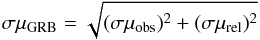 (13)allows us to build the Combo-GRB Hubble diagram (see also Izzo et al. 2009), which is shown in Fig. 5. It is possible to quantify the reliability of any cosmological model with our sample of 60 GRBs, which represents a unique dataset from low redshift (z = 0.145) to very large distances (z = 8.23). To reach our goal, we make the fundamental assumption that our GRB sample is normally distributed around the best-fit cosmology, which we are going to estimate. With this hypothesis, we consider as test-statistic the chi-square test, which is defined as
 ![Mathematical equation: \begin{equation} \label{eq:no16} \chi^2 = \sum_{i\,=\,1}^{60} \frac{\left[\mu_{{\rm GRB},i}(z, \mathcal{A}, \psi) - \mu_{\rm th}(z, \Omega_{\rm m}, \Omega_{\Lambda}, w(z))\right]^2}{\sigma \mu_{{\rm GRB},i}^2}, \end{equation}](/articles/aa/full_html/2015/10/aa26461-15/aa26461-15-eq154.png) (14)where
(14)where  , μth(z,Ωm,ΩΛ,w(z)), and σμGRB are respectively defined in Eqs. (10), (11), and (13). The cosmology is included in the quantity μth(z,Ωm,ΩΛ,H0), which we allow to vary. To determine the best configuration of parameters that most closely fits the distribution of GRBs in the Hubble diagram we maximize the log-likelihood function, −2ln(eχ2), which is equivalent to the minimization of the function defined in Eq. (14).
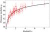 |
Fig. 5 Combo-GRB Hubble diagram. The black line represents the best fit for the function μ(z) as obtained by using only GRBs and for the case of the ΛCDM scenario. |
4.2. Fit results
4.2.1. ΛCDM case
In the ΛCDMmodel, the energy function E(z,Ωm,ΩΛ,w(z)) is characterized by an EOS for the dark energy term fixed to w = −1. Since we have that Ωm + ΩΛ + Ωk = 1, we vary the matter and cosmological constant density parameters, also obtaining in this way an estimate of the curvature term. We obtain that GRBs alone provide  , see also Fig. 6.
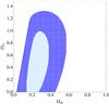 |
Fig. 6 1σ(Δχ2 = 2.3) confidence region in the (Ωm, ΩΛ) plane for the Combo-GRB sample (dark blue), and for the total (60 observed + 300 MC simulated GRBs, (light blue). |
4.2.2. Variable w0 case
In a flat Universe (Ω = Ωm + ΩΛ = 1) with a constant value of w0 different from the standard value w = −1, we can provide useful constraints for alternative dark energy theories. In this case, we only vary the matter density and the dark energy equations of state, obtaining an estimate of the density matter of  and of a dark energy EOS parameter
  .
.
4.2.3. Evolution of w(z)
An interesting case-study consists of a time-evolving dark energy EOS in a flat cosmology, since the evolution of w(z) can be directly studied with GRBs at larger redshifts. We consider an analytical formulation for the evolution of w with the redshift, which was proposed by Chevallier & Polarski (2001) and Linder (2003) (CPL), and where the w(z) can be parameterized by 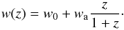 (15)The CPL parameterization implies that for large z the w(z) term tends to the asymptotic value w0 + wa. Using a sample extending at large redshifts, e.g. GRBs, will allow a better estimate of these parameters since the effects of a varying w(z) on the distance modulus are more evident at redshift z ≥ 1. The GRB data provide a best-fit result
  .
.
4.2.4. Perspective: a Monte Carlo simulated sample of GRBs
The current sample of GRBs that satisfies the Combo-relation is quite limited (60 bursts), when compared to the sample in Amati & Della Valle (2013) (~200 bursts) or the SNe sample in the Union 2.1 release (Suzuki et al. 2012). A more numerous sample can help to understand whether the Combo-relation can provide better constraints on the cosmological parameters. To this aim, following the prescription of Li (2007), we used Monte Carlo (MC) simulations to generate a sample of 300 synthetic GRBs satisfying the Combo-relation. This value comes from the expected number of GRBs detected in five years of operations of current (Swift) and future (SVOM, Gotz et al. 2009, and LOFT, Feroci et al. 2012) missions dedicated to observing GRBs.
First, we fitted the log-normal distributions of the 60 observed z, Ep,i, τ, and | α + 1 |, ![Mathematical equation: \begin{equation} \label{eq:lognormal} f(\log \xi) = \frac{1}{\sqrt{2\pi}\sigma_\xi}\exp\left[-\frac{\left(\log \xi-\mu_\xi\right)^2}{2\sigma_\xi^2}\right]\ , \end{equation}](/articles/aa/full_html/2015/10/aa26461-15/aa26461-15-eq180.png) (16)where ξ = z, Ep,i, τ, and | α + 1 |, and we found the following mean values and dispersions: μz ± σz = 0.26 ± 0.27, μEp,i ± σEp,i = 2.54 ± 0.40, μτ ± στ = 2.85 ± 0.65, and μ| α + 1 | ± σ| α + 1 | = −0.36 ± 0.31. Then, from these distributions we computed log X(γ,Ep.i,τ,α) and we generated the initial luminosity log L0 = γlog X + A from the frequency distribution
(16)where ξ = z, Ep,i, τ, and | α + 1 |, and we found the following mean values and dispersions: μz ± σz = 0.26 ± 0.27, μEp,i ± σEp,i = 2.54 ± 0.40, μτ ± στ = 2.85 ± 0.65, and μ| α + 1 | ± σ| α + 1 | = −0.36 ± 0.31. Then, from these distributions we computed log X(γ,Ep.i,τ,α) and we generated the initial luminosity log L0 = γlog X + A from the frequency distribution ![Mathematical equation: \begin{equation} f(\log L_0) = \frac{1}{\sqrt{2\pi}\sigma_{\rm ext}}\exp\left[-\frac{\left(\log L_0 - \gamma \log X -A \right)^2}{2\sigma_{\rm ext}^2}\right] , \end{equation}](/articles/aa/full_html/2015/10/aa26461-15/aa26461-15-eq188.png) (17)assuming that the Combo-relation is independent of the redshift and considering its extra-scatter σext. The values of γ, A, and σext are reported in Sect. 3. Finally, to complete the set of parameters necessary to compute the distance modulus of the simulated sample of GRBs from each pair (log L0, z), we generated the corresponding log F0 (μF0 ± σF0 = −9.87 ± 0.85). In the following, the attached errors on the MC simulated Combo-relation parameters will be taken as 30% of their corresponding values, which reflects the uncertainty of the “real” GRB sample.
(17)assuming that the Combo-relation is independent of the redshift and considering its extra-scatter σext. The values of γ, A, and σext are reported in Sect. 3. Finally, to complete the set of parameters necessary to compute the distance modulus of the simulated sample of GRBs from each pair (log L0, z), we generated the corresponding log F0 (μF0 ± σF0 = −9.87 ± 0.85). In the following, the attached errors on the MC simulated Combo-relation parameters will be taken as 30% of their corresponding values, which reflects the uncertainty of the “real” GRB sample.
We have verified whether the constraints on (Ωm, ΩΛ) will improve by using a larger sample of 360 GRBs (the real sample of 60 GRBs observed and a MC-simulated sample of 300 GRBs, described above). The improvement on the constraints on Ωm and ΩΛ is clear: the uncertainties on the density parameters improve considerably ( for the ΛCDM case,
  for the variable w0 case), as is also clear in the contour plots shown in Figs. 6 and 7.
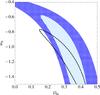 |
Fig. 7 1σ(Δχ2 = 2.3) confidence region in the (Ωm, w0) plane for the Combo-GRB sample (dark blue), and for the total of 60 observed + 300 MC simulated GRBs (light blue). The black dashed line represents the 1σ confidence region obtained using the recent Union 2.1 SNe Ia sample (Suzuki et al. 2012). |
4.3. GRBs compared with SNe, CMBs, BAOs
In order to compare the Combo-GRB sample results, we also consider the following datasets:
-
The measurements of the baryon acoustic peaks Aobs = (0.474 ± 0.034,0.442 ± 0.020,0.424 ± 0.021) at the corresponding redshifts zBAO = (0.44,0.6,0.73) in the galaxy correlation function as obtained by the WiggleZ dark energy Survey (Blake et al. 2011). The BAO peak is defined as (Eisenstein et al. 2005)
![Mathematical equation: \begin{equation} \label{eq:no17} A_{\rm BAO} = \left[ \frac{cz_{\rm BAO}}{H_0}\frac{r(z_{\rm BAO},\Omega_{\rm m},\Omega_\Lambda,w(z))^2}{E(z,\Omega_{\rm m},\Omega_\Lambda,w(z))}\right]^{1/3} \frac{\sqrt{\Omega_{\rm m} H_0^2}}{c z_{\rm BAO}} , \end{equation}](/articles/aa/full_html/2015/10/aa26461-15/aa26461-15-eq197.png) (18)where
r(z,Ωm,ΩΛ,w(z))
is the comoving distance. The best-fit cosmological model is determined by the
minimization of the corresponding chi-squared quantity
(18)where
r(z,Ωm,ΩΛ,w(z))
is the comoving distance. The best-fit cosmological model is determined by the
minimization of the corresponding chi-squared quantity 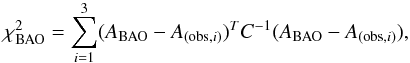 (19)where
C-1 is the inverse covariance matrix
of the measurements of the WiggleZ survey (Blake et
al. 2011).
(19)where
C-1 is the inverse covariance matrix
of the measurements of the WiggleZ survey (Blake et
al. 2011). -
The measurement of the shift parameter Robs = 1.7407 ± 0.0094 as obtained from the Planck first data release (Planck Collaboration XVI 2014). The R quantity is the least cosmological model-dependent parameter (particularly from H0) that can be extracted from the analysis of the CMB (Wang & Mukherjee 2006) and is defined as
 (20)where
zrec is the redshift of the
recombination. The best-fit cosmological model is determined by the minimization of
the corresponding chi-squared term
(20)where
zrec is the redshift of the
recombination. The best-fit cosmological model is determined by the minimization of
the corresponding chi-squared term  (21)
(21)
 values for any pair of parameters and for the combined values,
  (22)and make the final plots using the Mathematica1 software suite. Cosmological parameter uncertainties were estimated from single and combined χ2 statistics for each dataset. In Fig. 8 we show the parameter spaces with the contour at the 1σ (Δχ2 = 2.3) confidence limit for each considered dataset, and for the ΛCDM case. We note that in all the datasets and fits, the Hubble constant is fixed to the value of H0 = 70.6 ± 2.6 (Rigault et al. 2014). From the combination of all the considered datasets, for the ΛCDM case, we obtain a matter density value of
  , which shows no strain with the Combo-GRB results and the simulated one, see Fig. 8.
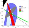 |
Fig. 8 1σ(Δχ2 = 2.3) confidence region in the (Ωm, ΩΛ) plane for the observed GRB sample (blue), with the inclusion of the MC-simulated 300 GRBs sample (cyan), and with the samples of SNe (grey), BAOs (red), and CMBs (green). The dashed line represents the condition of the Flat Universe Ωm + ΩΛ = 1. |
5. Discussions and conclusions
In this paper we have presented the “Combo” relation, a new tool for GRB cosmology. This relationship provides a very close link between prompt and afterglow parameters and it is characterized by a small intrinsic scatter, which makes this correlation very suitable for cosmological purposes. We recognize the fundamental role of the Swift-XRT (Gehrels et al. 2004; Burrows et al. 2005) which, thanks to its ability to slew very rapidly toward the location of a GRB event, provides real-time and detailed data of GRB afterglow light curves, whose evolution is at the base of the proposed Combo-relation. From our analysis the following results emerge:
-
The proposed two-step calibration of the Combo-GRB relation greatly minimizes the dependence on SNe Ia.
-
GRBs data alone provide for the ΛCDM case
, see Fig. 8. -
A recent paper (Milne et al. 2015) highlights the existence of an observational bias (a systematic difference in the velocity of SNe Ia ejecta, which is reflected in their curves), potentially affecting the measurements of cosmological parameters obtained with SNe Ia. On the basis of our results we conclude that given the current accuracy of GRB measurements we cannot exclude, within the errors, that an effect like this is at play; however, this effect should not change the conclusions derived from SNe-Ia observations.
-
The launch of advanced and more sensitive detectors, such as the incoming SVOM (Gotz et al. 2009) and the proposed LOFT (Feroci et al. 2012) missions (and the expected Swift operations in the near future), will dramatically increase the number of GRBs in the dataset. In five years of operation of the SVOM mission alone, we expect to reach a “good enough” sample of 300 GRBs. With a Monte Carlo simulated sample of 300 GRBs, we will significantly improve the accuracy of Ωm measurement, up to
, which is comparable with type Ia SNe (Suzuki et al. 2012). -
By using the CPL analytical parameterization, adopted to study the evolution of the dark energy EOS (see Eq. (15)), we find
,  , and
, and  .
. -
The analysis of a combined (SNe+BAO+CMB) dataset confirms that the increasing size of the GRB sample will improve the accuracy of the measurement of the Ωm parameter and in particular of the evolution of w up to z ~ 10.
-
The analytical expression of the Combo-relation provides an explicit close link, characterized by a small intrinsic scatter, between the prompt and the afterglow GRB emissions. This points out the existence of a physical connection between the prompt and the afterglow emissions, which represents a new challenge for GRB models.
Interactive Data Language, http://www.exelisvis.com/language/en-US/ProductsServices/IDL.aspx
Acknowledgments
We thank the referee for her/his constructive comments which have improved the paper. E.Z. acknowledges the support by the International Cooperation Program CAPES-ICRANet financed by CAPES – Brazilian Federal Agency for Support and Evaluation of Graduate Education within the Ministry of Education of Brazil. This work made use of data supplied by the UK Swift Science Data Centre at the University of Leicester.
References
- Amanullah, R., Lidman, C., Rubin, D., et al. 2010, ApJ, 716, 712 [NASA ADS] [CrossRef] [Google Scholar]
- Amati, L., & Della Valle, M. 2013, Int. J. Mod. Phys. D, 22, 30028 [Google Scholar]
- Amati, L., Frontera, F., Tavani, M., et al. 2002, A&A, 390, 81 [NASA ADS] [CrossRef] [EDP Sciences] [Google Scholar]
- Amati, L., Guidorzi, C., Frontera, F., et al. 2008, MNRAS, 391, 577 [NASA ADS] [CrossRef] [MathSciNet] [Google Scholar]
- Bernardini, M. G., Bianco, C. L., Caito, L., et al. 2007, A&A, 474, L13 [NASA ADS] [CrossRef] [EDP Sciences] [Google Scholar]
- Bernardini, M. G., Margutti, R., Zaninoni, E., & Chincarini, G. 2012, MNRAS, 425, 1199 [NASA ADS] [CrossRef] [Google Scholar]
- Blake, C., Kazin, E. A., Beutler, F., et al. 2011, MNRAS, 418, 1707 [NASA ADS] [CrossRef] [MathSciNet] [Google Scholar]
- Bronstein, M. P. 1933, Phys. Z. Sowjetunion, 3, 73 [Google Scholar]
- Burrows, D., Hill, J., Nousek, J., et al. 2005, Space Sci. Rev., 120, 165 [NASA ADS] [CrossRef] [Google Scholar]
- Caito, L., Amati, L., Bernardini, M. G., et al. 2010, A&A, 521, A80 [NASA ADS] [CrossRef] [EDP Sciences] [Google Scholar]
- Capozziello, S., & Izzo, L. 2008, A&A, 490, 31 [NASA ADS] [CrossRef] [EDP Sciences] [Google Scholar]
- Chevallier, M., & Polarski, D. 2001, Int. J. Mod. Phys. D, 10, 213 [NASA ADS] [CrossRef] [Google Scholar]
- Coward, D. M., Howell, E. J., Branchesi, M., et al. 2013, MNRAS, 432, 2141 [NASA ADS] [CrossRef] [Google Scholar]
- Cucchiara, A., Levan, A. J., Fox, D. B., et al. 2011, ApJ, 736, 7 [NASA ADS] [CrossRef] [Google Scholar]
- D’Agostini, G. 2005, ArXiv e-prints [arXiv:physics/0511182] [Google Scholar]
- Dai, Z. G., Liang, E. W., & Xu, D. 2004, ApJ, 612, L101 [NASA ADS] [CrossRef] [Google Scholar]
- Dainotti, M. G., Cardone, V. F., & Capozziello, S. 2008, MNRAS, 391, L79 [NASA ADS] [CrossRef] [Google Scholar]
- de Bernardis, P., Ade, P. A. R., Bock, J. J., et al. 2000, Nature, 404, 955 [NASA ADS] [CrossRef] [PubMed] [Google Scholar]
- D’Elia, V., Fiore, F., Meurs, E. J. A., et al. 2007, A&A, 467, 629 [NASA ADS] [CrossRef] [EDP Sciences] [Google Scholar]
- Demianski, M., Piedipalumbo, E., Rubano, C., & Scudellaro, P. 2012, MNRAS, 426, 1396 [NASA ADS] [CrossRef] [Google Scholar]
- Eisenstein, D. J., Zehavi, I., Hogg, D. W., et al. 2005, ApJ, 633, 560 [NASA ADS] [CrossRef] [Google Scholar]
- Feroci, M., den Herder, J. W., Bozzo, E., et al. 2012, in SPIE Conf. Ser., 8443 [Google Scholar]
- Firmani, C., Ghisellini, G., Avila-Reese, V., & Ghirlanda, G. 2006, MNRAS, 370, 185 [NASA ADS] [CrossRef] [Google Scholar]
- Gehrels, N., Chincarini, G., Giommi, P., et al. 2004, ApJ, 611, 1005 [NASA ADS] [CrossRef] [Google Scholar]
- Ghirlanda, G., Ghisellini, G., & Lazzati, D. 2004, ApJ, 616, 331 [NASA ADS] [CrossRef] [Google Scholar]
- Ghirlanda, G., Ghisellini, G., & Firmani, C. 2006, New J. Phys., 8, 123 [NASA ADS] [CrossRef] [Google Scholar]
- Goobar, A., & Perlmutter, S. 1995, ApJ, 450, 14 [NASA ADS] [CrossRef] [Google Scholar]
- Gotz, D., Paul, J., Basa, S., et al. 2009, in AIP Conf. Ser. 1133, eds. C. Meegan, C. Kouveliotou, & N. Gehrels, 25 [Google Scholar]
- Guy, J., Astier, P., Baumont, S., et al. 2007, A&A, 466, 11 [NASA ADS] [CrossRef] [EDP Sciences] [Google Scholar]
- Izzo, L., Capozziello, S., Covone, G., & Capaccioli, M. 2009, A&A, 508, 63 [NASA ADS] [CrossRef] [EDP Sciences] [Google Scholar]
- Kalberla, P. M. W., Burton, W. B., Hartmann, D., et al. 2005, A&A, 440, 775 [NASA ADS] [CrossRef] [EDP Sciences] [Google Scholar]
- Kodama, Y., Yonetoku, D., Murakami, T., et al. 2008, MNRAS, 391, L1 [NASA ADS] [CrossRef] [Google Scholar]
- Li, L.-X. 2007, MNRAS, 379, L55 [NASA ADS] [CrossRef] [Google Scholar]
- Liang, E., & Zhang, B. 2006, MNRAS, 369, L37 [NASA ADS] [CrossRef] [Google Scholar]
- Linder, E. V. 2003, Phys. Rev. Lett., 90, 091301 [NASA ADS] [CrossRef] [PubMed] [Google Scholar]
- Lloyd, N. M., & Petrosian, V. 1999, ApJ, 511, 550 [NASA ADS] [CrossRef] [Google Scholar]
- Macpherson, D., Coward, D. M., & Zadnik, M. G. 2013, ApJ, 779, 73 [NASA ADS] [CrossRef] [Google Scholar]
- Mannucci, F., Della Valle, M., & Panagia, N. 2006, MNRAS, 370, 773 [NASA ADS] [CrossRef] [Google Scholar]
- Margutti, R., Guidorzi, C., Chincarini, G., et al. 2010, MNRAS, 406, 2149 [NASA ADS] [CrossRef] [Google Scholar]
- Margutti, R., Chincarini, G., Granot, J., et al. 2011, MNRAS, 417, 2144 [NASA ADS] [CrossRef] [Google Scholar]
- Margutti, R., Zaninoni, E., Bernardini, M. G., et al. 2013, MNRAS, 428, 729 [NASA ADS] [CrossRef] [Google Scholar]
- Markwardt, C. B. 2009, in Astronomical Data Analysis Software and Systems XVIII, eds. D. A. Bohlender, D. Durand, & P. Dowler, ASP Conf. Ser., 411, 251 [Google Scholar]
- Milne, P. A., Foley, R. J., Brown, P. J., & Narayan, G. 2015, ApJ, 803, 20 [NASA ADS] [CrossRef] [Google Scholar]
- Norris, J. P., & Bonnell, J. T. 2006, ApJ, 643, 266 [NASA ADS] [CrossRef] [Google Scholar]
- Norris, J. P., Marani, G. F., & Bonnell, J. T. 2000, ApJ, 534, 248 [NASA ADS] [CrossRef] [Google Scholar]
- Nousek, J. A., Kouveliotou, C., Grupe, D., et al. 2006, ApJ, 642, 389 [NASA ADS] [CrossRef] [Google Scholar]
- Perlmutter, S., Aldering, G., della Valle, M., et al. 1998, Nature, 391, 51 [CrossRef] [Google Scholar]
- Perlmutter, S., Aldering, G., Goldhaber, G., et al. 1999, ApJ, 517, 565 [NASA ADS] [CrossRef] [Google Scholar]
- Pisani, G. B., Izzo, L., Ruffini, R., et al. 2013, A&A, 552, L5 [NASA ADS] [CrossRef] [EDP Sciences] [Google Scholar]
- Planck Collaboration XVI. 2014, A&A, 571, A16 [NASA ADS] [CrossRef] [EDP Sciences] [Google Scholar]
- Planck Collaboration XIII. 2015, A&A, submitted [arXiv:1502.01589] [Google Scholar]
- Ramirez-Ruiz, E., & Fenimore, E. E. 2000, ApJ, 539, 712 [NASA ADS] [CrossRef] [Google Scholar]
- Reichart, D. E., Lamb, D. Q., Fenimore, E. E., et al. 2001, ApJ, 552, 57 [NASA ADS] [CrossRef] [Google Scholar]
- Riess, A. G., Filippenko, A. V., Challis, P., et al. 1998, AJ, 116, 1009 [NASA ADS] [CrossRef] [Google Scholar]
- Rigault, M., Aldering, G., Kowalski, M., et al. 2015, ApJ, 802, 20 [NASA ADS] [CrossRef] [Google Scholar]
- Robertson, B. E., & Ellis, R. S. 2012, ApJ, 744, 95 [NASA ADS] [CrossRef] [Google Scholar]
- Ruffini, R., Muccino, M., Bianco, C. L., et al. 2014, A&A, 565, L10 [NASA ADS] [CrossRef] [EDP Sciences] [Google Scholar]
- Salvaterra, R., Della Valle, M., Campana, S., et al. 2009, Nature, 461, 1258 [NASA ADS] [CrossRef] [PubMed] [Google Scholar]
- Schaefer, B. E. 2007, ApJ, 660, 16 [NASA ADS] [CrossRef] [Google Scholar]
- Schmidt, B. P., Suntzeff, N. B., Phillips, M. M., et al. 1998, ApJ, 507, 46 [NASA ADS] [CrossRef] [Google Scholar]
- Suzuki, N., Rubin, D., Lidman, C., et al. 2012, ApJ, 746, 85 [NASA ADS] [CrossRef] [Google Scholar]
- Tanvir, N. R., Fox, D. B., Levan, A. J., et al. 2009, Nature, 461, 1254 [NASA ADS] [CrossRef] [PubMed] [Google Scholar]
- Trenti, M., Perna, R., & Tacchella, S. 2013, ApJ, 773, L22 [NASA ADS] [CrossRef] [Google Scholar]
- Trenti, M., Perna, R., & Jimenez, R. 2015, ApJ, 802, 103 [NASA ADS] [CrossRef] [Google Scholar]
- Tsutsui, R., Nakamura, T., Yonetoku, D., et al. 2009, J. Cosmol. Astropart. Phys., 8, 15 [NASA ADS] [CrossRef] [Google Scholar]
- Wang, Y., & Mukherjee, P. 2006, ApJ, 650, 1 [NASA ADS] [CrossRef] [Google Scholar]
- Wang, F. Y., Dai, Z. G., Liang, E. W. 2015, New A Rev., 67, 1 [Google Scholar]
- Wei, J.-J., Wu, X.-F., Melia, F., Wei, D.-M., & Feng, L.-L. 2014, MNRAS, 439, 3329 [NASA ADS] [CrossRef] [Google Scholar]
- Willingale, R., O’Brien, P. T., Osborne, J. P., et al. 2007, ApJ, 662, 1093 [NASA ADS] [CrossRef] [Google Scholar]
- Yonetoku, D., Murakami, T., Nakamura, T., et al. 2004, ApJ, 609, 935 [NASA ADS] [CrossRef] [Google Scholar]
- Zaninoni, E. 2013, Ph.D. Thesis, http://paduaresearch.cab.unipd.it/5626/ [Google Scholar]
- Zhang, B., Fan, Y. Z., Dyks, J., et al. 2006, ApJ, 642, 354 [NASA ADS] [CrossRef] [Google Scholar]
Appendix A: Computation of the rest-frame 0.3–10 keV luminosity L(t )
)
The rest-frame 0.3–10 keV luminosity was obtained by considering four steps.
-
(1)
We obtained the Swift-XRT flux light curves in the observed 0.3–10 keV energy band2.
-
(2)
We transformed the observed flux fobs from the observed energy band 0.3–10 keV to the rest-frame energy band 0.3–10 keV by assuming an absorbed power-law function as the best fit for the spectral energy distribution of the XRT data, N(E) ~ E− γ, with Galactic and intrinsic column densities obtained from the H i radio map (Kalberla et al. 2005) and from the best fit of the total afterglow spectrum, respectively. By using the photon indexes inferred for each time interval, the rest-frame flux light curve frf is given by
 (A.1)
(A.1) -
(3)
We transformed the observed time ta into the rest-frame time by correcting for z
 (A.2)
(A.2) -
(4)
We defined the isotropic luminosity as
 (A.3)
(A.3)
Appendix B: Determination of the sample and verification of the correlation
To obtain the parameters involved in the Eq. (5), we needed to select an adequate sample of GRBs, to fit their X-ray light curves, and to collect or to calculate their Ep,i values. The selection criteria have already been delineated in Sect. 2.
The entire procedure works in the rest-frame 0.3–10 keV energy range for all GRBs. For the X-ray light curve fitting technique we developed a semi-automated code performing all the needed operations. The code is based on the IDL3 language, and the fitting routine used is MPFIT4 (Markwardt 2009), which is based on the non-linear least squares fitting. First, the procedure fits the complete light curve, then it eliminates at every iteration the data point with the largest positive residual, until it obtains a fit with a p-value greater than 0.3. To fit the light curves considered in luminosity units (erg/s), we use the composite function (R14):
-
1.
a power law for the early steep decay
 (B.1)with Lp the normalization factor and αp the slope;
 -
2.
Eq. (3) for the afterglow additional component.
An application of this joint fitting procedure is shown in Fig. B.1 for the case of GRB 060418. After the fitting procedure, we select only the GRBs with αX< −1, a condition necessary for the convergence of the integral in Eq. (4). The final total sample, summarized in Table B.1, consists of 60 GRBs.
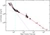 |
Fig. B.1 Example of the combined fitting procedure (solid red line) as described in Eqs. (3) and (B.1), filtered by the flares. The early steep decay fitted by using the power-law function in Eq. (B.1) is indicated by the purple dashed line, while the afterglow additional component is fitted by the phenomenological function in Eq. (3) (see also R14), and described by the dot-dashed cyan curve. In this specific case, the luminosity light curve of GRB 060418 is shown in which the black dots with the error bars are the flare-free data, the grey dots are the excluded data recognized as due to the flares. The vertical green dotted line indicates the characteristic timescale of the parameter τ. |
Long bursts with αX< −1 analysed in this work (first column) and their main parameters.
All Tables
Five GRBs used for the determination of the slope parameter γ of the correlation.
Five SNe Ia selected from the Union2 sample (Amanullah et al. 2010; Suzuki et al. 2012) and used for the calibration of the GRB correlation.
Long bursts with αX< −1 analysed in this work (first column) and their main parameters.
All Figures
|
Fig. 1 EX,iso–Eγ,iso–Ep,i correlation proposed by Bernardini et al. (2012) and Margutti et al. (2013) (courtesy R. Margutti). |
| In the text | |
|
Fig. 2 Correlation considering the entire sample of 60 GRBs. The green empty boxes are the data of each of the sources, derived as described in Appendix B, the solid black line is the best fit of the data, while the dotted grey lines and the dashed grey lines correspond, respectively, to the dispersion on the correlation at 1σex and 3σex. |
| In the text | |
|
Fig. 3 Residual distance modulus μobs − μth for different values of the density cosmological parameters Ωm and ΩΛ up to z = 2.0. We consider the best fit to be the standard ΛCDM model, where Ωm = 0.27, ΩΛ = 0.73, and H0 = 71 km s-1/Mpc (black line). Union2 SNe Ia data residuals are shown in grey. The large spread (more than 1 mag) shown by μ at z = 1.5 and at z = 0.145 (the two vertical dashed lines) where the scatter is almost 0.2 mag is clearly evident. |
| In the text | |
|
Fig. 4 Correlation found for the sample of five GRBs located at the same redshift. The blue triangles are the data of each of the five sources, derived from the procedure in Appendix B. The solid line represents the best fit while the dashed line is the dispersion on the correlation at 1σex. |
| In the text | |
|
Fig. 5 Combo-GRB Hubble diagram. The black line represents the best fit for the function μ(z) as obtained by using only GRBs and for the case of the ΛCDM scenario. |
| In the text | |
|
Fig. 6 1σ(Δχ2 = 2.3) confidence region in the (Ωm, ΩΛ) plane for the Combo-GRB sample (dark blue), and for the total (60 observed + 300 MC simulated GRBs, (light blue). |
| In the text | |
|
Fig. 7 1σ(Δχ2 = 2.3) confidence region in the (Ωm, w0) plane for the Combo-GRB sample (dark blue), and for the total of 60 observed + 300 MC simulated GRBs (light blue). The black dashed line represents the 1σ confidence region obtained using the recent Union 2.1 SNe Ia sample (Suzuki et al. 2012). |
| In the text | |
|
Fig. 8 1σ(Δχ2 = 2.3) confidence region in the (Ωm, ΩΛ) plane for the observed GRB sample (blue), with the inclusion of the MC-simulated 300 GRBs sample (cyan), and with the samples of SNe (grey), BAOs (red), and CMBs (green). The dashed line represents the condition of the Flat Universe Ωm + ΩΛ = 1. |
| In the text | |
|
Fig. B.1 Example of the combined fitting procedure (solid red line) as described in Eqs. (3) and (B.1), filtered by the flares. The early steep decay fitted by using the power-law function in Eq. (B.1) is indicated by the purple dashed line, while the afterglow additional component is fitted by the phenomenological function in Eq. (3) (see also R14), and described by the dot-dashed cyan curve. In this specific case, the luminosity light curve of GRB 060418 is shown in which the black dots with the error bars are the flare-free data, the grey dots are the excluded data recognized as due to the flares. The vertical green dotted line indicates the characteristic timescale of the parameter τ. |
| In the text | |
Current usage metrics show cumulative count of Article Views (full-text article views including HTML views, PDF and ePub downloads, according to the available data) and Abstracts Views on Vision4Press platform.
Data correspond to usage on the plateform after 2015. The current usage metrics is available 48-96 hours after online publication and is updated daily on week days.
Initial download of the metrics may take a while.