| Issue |
A&A
Volume 582, October 2015
|
|
|---|---|---|
| Article Number | A85 | |
| Number of page(s) | 13 | |
| Section | Stellar structure and evolution | |
| DOI | https://doi.org/10.1051/0004-6361/201526085 | |
| Published online | 13 October 2015 | |
Rotation period distribution of CoRoT⋆ and Kepler Sun-like stars
1
Departamento de FísicaUniversidade Federal do Rio Grande do
Norte,
Natal,
59072-970
RN,
Brazil
e-mail:
This email address is being protected from spambots. You need JavaScript enabled to view it.
2
ESO – European Southern Observatory, Karl-Schwarzschild-Strasse 2, 85748
Garching bei München,
Germany
3
SUPA (Scottish Universities Physics Alliance) Wide-Field Astronomy
Unit, Institute for Astronomy, School of Physics and Astronomy, University of
Edinburgh, Royal Observatory, Blackford Hill, Edinburgh
EH9 3HJ,
UK
4
Pontificia Universidad Católica de Chile, Instituto de
Astrofísica, Facultad de Física, Av. Vicuña Mackena 4860, 782-0436 Macul, Santiago, Chile
5
Pontificia Universidad Católica de Chile, Centro de Astroingeniería,
Av. Vicuña Mackena
4860, 782-0436 Macul, 7820436 Macul, Santiago, Chile
6
Millennium Institute of Astrophysics, Santiago, Chile
7
Universidade de São Paulo/IAG-USP, rua do Matão, 1226, Cidade
Universitária, 05508-900
São Paulo, SP, Brazil
8
LESIA, UMR 8109 CNRS, Observatoire de Paris, UVSQ, Université
Paris-Diderot, 5 place J.
Janssen, 92195
Meudon,
France
Received: 12 March 2015
Accepted: 4 September 2015
Abstract
Aims. We study the distribution of the photometric rotation period (Prot), which is a direct measurement of the surface rotation at active latitudes, for three subsamples of Sun-like stars: one from CoRoT data and two from Kepler data. For this purpose, we identify the main populations of these samples and interpret their main biases specifically for a comparison with the solar Prot.
Methods. Prot and variability amplitude (A) measurements were obtained from public CoRoT and Kepler catalogs, which were combined with public data of physical parameters. Because these samples are subject to selection effects, we computed synthetic samples with simulated biases to compare with observations, particularly around the location of the Sun in the Hertzsprung-Russel (HR) diagram. Publicly available theoretical grids and empirical relations were used to combine physical parameters with Prot and A. Biases were simulated by performing cutoffs on the physical and rotational parameters in the same way as in each observed sample. A crucial cutoff is related with the detectability of the rotational modulation, which strongly depends on A.
Results. The synthetic samples explain the observed Prot distributions of Sun-like stars as having two main populations: one of young objects (group I, with ages younger than ~1 Gyr) and another of main-sequence and evolved stars (group II, with ages older than ~1 Gyr). The proportions of groups I and II in relation to the total number of stars range within 64–84% and 16–36%, respectively. Hence, young objects abound in the distributions, producing the effect of observing a high number of short periods around the location of the Sun in the HR diagram. Differences in the Prot distributions between the CoRoT and Kepler Sun-like samples may be associated with different Galactic populations. Overall, the synthetic distribution around the solar period agrees with observations, which suggests that the solar rotation is normal with respect to Sun-like stars within the accuracy of current data.
Key words: stars: rotation / stars: evolution / stars: solar-type / Sun: rotation
The CoRoT space mission was developed and is operated by the French space agency CNES, with the participation of ESA’s RSSD and Science Programmes, Austria, Belgium, Brazil, Germany, and Spain.
© ESO, 2015
1. Introduction
A question of high interest is how exactly the Sun will evolve and, as a consequence, how it will affect the planetary environment. Although the Sun’s evolution has long been modeled from thermonuclear reaction rates, explaining non-canonical effects, such as sunspots and magnetic fields, is still puzzling. Clearly understanding the solar structure and evolution is necessary to know, for example, how long our central star will maintain the conditions required for life in the solar system, or whether its magnetic activity can damage our technological needs, among other concerns (e.g., Melott & Thomas 2011; Jones 2013; Shibata et al. 2013; Steinhilber & Beer 2013). To accurately predict the near and distant future characteristics of the Sun, it is essential to understand its past and project its future by studying other stars (e.g., Charbonneau 2010, 2013; Ekström et al. 2012). Specifically, stars with a similar mass and chemistry to that of the Sun may provide important constraints for the theoretical models used in predicting the Sun’s history (e.g., Schuler et al. 2011; Datson et al. 2012). To refine these models, stellar rotation is fundamental because this parameter is a key feature in controlling the root-cause of the structure, evolution, chemistry, and magnetism of the stars (e.g., Palacios 2013; Maeder & Meynet 2015). In particular, the measure of the surface rotation can substantially improve observational constraints on theory from a proper modeling of the stellar interior (e.g., Zahn 1992; Ekström et al. 2012; Brun et al. 2014). Further refinements can be obtained from the internal rotation, which has recently been measured in the Sun and several different types of stars thanks to remarkable advances in asteroseismology (e.g., Goupil et al. 2013; Deheuvels et al. 2014).
Another key question is how similar or different the Sun is compared to Sun-like stars, and rotation may also be crucial in this comparison (e.g., Gustafsson 1998; Gonzalez 1999, 2001). Different studies have discussed whether the Sun rotates normally with respect to its Sun-like counterparts, at least considering the surface rotation. For example, Soderblom (1983) and Gray (1982) suggested that the Sun rotates normally for its age, a finding corroborated by Robles et al. (2008). However, as reported by de Freitas et al. (2013), these studies were based on the projected rotational velocity (vsini), which is an indirect rotation measurement with the intrinsically unknown axis orientation angle i. In contrast, Metcalfe et al. (2013) found in a recent study of magnetic activity cycles of the solar analog ϵ Eri that this star undergoes long-term magnetic cycles compatible with those of the Sun, but the rotation period Prot determined from the photometric time-series (e.g., Strassmeier 2009) is approximately twice as fast. Based on Prot, which is a direct measurement of the surface rotation at the active latitudes, it is suggested that the Sun may rotate more slowly than its analogs. Nevertheless, the question about solar rotation normality remains unanswered, especially when we consider its rotation compared to direct stellar rotation measurements.
To date, most comparative studies of the Sun’s rotation relative to other stars are based on the projected rotational velocity from vsini (e.g., Porto de Mello & da Silva 1997; Meléndez et al. 2006), which, as explained, may hinder proper comparison. In contrast, the number of databases with direct Prot measurements from the photometric time-series is growing rapidly (e.g., Strassmeier et al. 2000; Strassmeier 2009; Hartman et al. 2010; De Medeiros et al. 2013; Reinhold et al. 2013; McQuillan et al. 2014). Current examples of databases with stellar rotation periods are those obtained from the CoRoT1 (Baglin et al. 2009) and Kepler2 (Koch et al. 2010) space telescope data, which include long-term light curves (LCs) with high-temporal resolution and high-photometric sensibility for more than 300 000 objects. Together, these databases include tens of thousands of period measurements of suggested rotation or candidates (e.g., Meibom et al. 2011; Affer et al. 2012, 2013; De Medeiros et al. 2013; Nielsen et al. 2013; McQuillan et al. 2013a,b, 2014; Reinhold et al. 2013; Walkowicz & Basri 2013). However, for many of these stars, no spectroscopic data are available. Thus, it is difficult to associate their periods with other physical parameters, such as metallicity, mass, radius, temperature, and age.
In particular, McQuillan et al. (2013a, 2014) found evidence of a bimodal Prot distribution for cool stars that becomes shallower with higher temperatures. Such a bimodality, also detected in Reinhold et al. (2013), has been proposed to originate from stellar populations that evolved differently from one another. The current lack of spectroscopic data is one of the main limitations in explaning this effect. The Kepler database so far provides photometric estimates of physical parameters for nearly all targets that are useful for several purposes. With regard to CoRoT, these photometric estimates are typically available for the targets of the asteroseismology channel. Thus, follow-up is crucial to obtain this physical information for the targets of the exoplanet channel (i.e., those considered in the present work).
Recently, García et al. (2014) examined the rotational evolution of solar-like stars based on the Kepler data. These authors performed a refined study of the age-rotation-activity relations by combining rotation period measurements with precise asteroseismic ages. One of the results was an analysis of the evolution of the rotation period as a function of stellar age for selected 12 cool dwarfs. The period-age relation corresponded well with previous calibrations, such as the Skumanich law (Skumanich 1972) and those obtained by Barnes (2007) and Mamajek & Hillenbrand (2008). Based on the referenced work, a fit with the 12 selected stars is compatible with the Sun location in the period-age diagram. However, the Sun lies at a slightly longer period than the fit, a small discrepancy that needs to be investigated in more detail.
For general studies of Kepler stars, Huber et al. (2014) provided a compilation of physical parameters obtained from different methods with improved values and well-computed errors by adjusting observational data with theoretical grids. For CoRoT targets, Sarro et al. (2013) recently published a relatively long list of physical parameters obtained automatically from spectroscopy. These data represent a unique opportunity for follow-up of the photometric periods determined from CoRoT and Kepler observations. In addition, a comparison between observations and theory can be performed by considering recent evolutionary models developed by the Geneva Team (Ekström et al. 2012), which account for stellar rotation based on a rich set of physical ingredients (see Sect. 3). Accordingly, photometric periods can be compared with these models. It is necessary for such a comparison to carefully analyze the observational bias of the observed sample, as described below.
Biases are typically modeled in stellar population synthesis, such as in the TRILEGAL3 (e.g., Girardi et al. 2005) and SYCLIST4 (Georgy et al. 2014) codes. TRILEGAL combines nonrotating evolutionary tracks with several ingredients, such as the star formation rate, age-metallicity relation, initial mass function, and geometry of Galaxy components, to simulate, in particular, the distribution of physical parameters and photometric measurements of different stellar populations. SYCLIST is a recent code developed by the Geneva Team that includes stellar rotation in a detailed set of ingredients to compute synthetic parent samples. The code considers anisotropies of the stellar surface, such as the latitude-dependence of temperature and luminosity and their effects on the limb darkening, to predict how the measured physical parameters can be affected by different rotation axis orientations. The resulting biases can, for example, affect the age estimation of coeval samples or of individual field stars because the physical parameters may deviate from their actual values. Although the SYCLIST code can be used to predict deviations on rotation measurements that are the result of different axis orientations, it does not yet consider the detectability of Prot measurements from LC variations.
For a deeper study of stellar rotation, understanding biases of Prot measurements can be particularly useful. As such, an important effect must be considered: the amplitude of the rotational modulation decreases as long as the stars evolve (e.g., Messina et al. 2001, 2003; Giampapa 2011; Spada et al. 2011); this decreases their detectability. As a consequence, current field stellar samples with Prot measurements are biased, exhibiting a lack of stars around the solar rotation period5. This bias hampers a proper analysis of the solar rotation normality regarding the Prot distribution of Sun-like field stars. Therefore, a quantified analysis is needed to better identify these biases in field stellar samples with variability measurements.
We here study the empirical distribution of Prot for field stars with physical parameters similar to those of the Sun. To this end, three different subsamples of Sun-like stars were obtained from the CoRoT and Kepler public catalogs, and synthetic samples were built by reproducing the main biases of the observed samples. Actual and synthetic samples can then be compared to one another to interpret the observational biases and to study the solar rotation normality. This analysis is performed by testing the most recent theoretical predictions combined with a large amount of new observational data. Combining this observational and theoretical information in the same analysis allows us to conduct an unprecedented study concerning these CoRoT and Kepler targets compared with the solar rotation.
We begin by describing our methods (Sect. 2) for sample selection from the public CoRoT and Kepler data. Next, we explain the methods we used to build the synthetic samples (Sect. 3). We discuss the rotation period distribution of young stars (Sect. 4), which were needed to constrain our synthetic samples. We present our results (Sect. 5) starting from the validation between the observational data and theoretical predictions for the Sun-like CoRoT sample. This sample, obtained from De Medeiros et al. (2013, hereafter DM13) was carefully considered as a catalog of rotating candidates because physical information of its sources was very limited during its development. Now, new spectroscopic physical parameters provided by Sarro et al. (2013) allow us to determine whether this sample is indeed a catalog of Prot. Finally, the Prot distribution is analyzed for the CoRoT and Kepler subsamples of Sun-like stars by interpreting biases and by comparing the stars with the solar rotation.
2. Sample selection and physical parameters
In this section, we summarize the catalogs used to obtain our observational samples, from which we constructed the corresponding synthetic samples. These include the CoRoT and Kepler catalogs with variability period measurements and those used to derive the physical parameters.
2.1. Selection of CoRoT targets and their parameters
From a parent sample of 124 471 LCs, DM13 presented a catalog of 4206 CoRoT stellar rotating candidates with unambiguous variability periods. A detailed procedure was developed for proper selection of the targets, based only on CoRoT LCs and 2MASS photometry, before additional data such as spectroscopy data were available. The procedure includes an automatic pre-selection of LCs that corrects them for jumps, long-term trends, and outliers, and identifies a preliminary list of periods, amplitudes (A), and signal-to-noise ratios (S/N). The variability period was computed from Lomb-Scargle (Lomb 1976; Scargle 1982; Horne & Baliunas 1986) periodograms, the amplitude from a harmonic fit of the phase diagram for the main period, and the S/N was the amplitude-to-noise ratio calculated from the LC. These parameters were then used to select the highest quality LCs (high S/N) in the expected amplitude and period ranges for rotating candidates. This criterion is related to the detectability of rotational modulation in an LC and was used in the present work as a relevant ingredient to produce a synthetic sample with biases (see Sect. 3). Finally, visual inspection was performed by applying a list of well-defined criteria for identifying photometric variability compatible with the rotational modulation caused by dynamic star spots (semi-sinusoidal variation6 defined in DM13), and the final parameters were refined.
Sarro et al. (2013) used neural networks similar to those employed in the CoRoT Variable Classifier (CVC) tool (Debosscher et al. 2007, 2009; Blomme et al. 2010) to obtain physical parameters from spectroscopic data of 6832 CoRoT targets. The method was applied to FLAMES/GIRAFFE7 spectra by using two different types of training sets. One is composed of synthetic spectra from Kurucz models (Bertone et al. 2008) and TLUSTY grids Hubeny & Lanz (1995; KT set) and the other of actual ELODIE8 spectra with known parameters from the ELODIE library (Prugniel & Soubiran 2001, 2004; ELODIE set). Physical parameters, particularly gravity (log g) and effective temperature (Teff), were then obtained independently for both sets. The main limitations of this catalog are the uncertainties in the computed parameters. Thus, no metallicity values are available and the errors in log g and Teff are relatively high (originally with typical values of approximately 0.5 dex and 400 K, respectively). As a first step to optimize our analysis despite the limitations, we averaged multiple independent estimations of log g and Teff provided by Sarro et al. (2013) for each target, which decreased the typical uncertainties slightly to approximately 0.4 dex and 300 K, respectively.
For the sample selection, we combined the catalog of DM13 with the available physical parameters given by Sarro et al. (2013). This provided a subsample of 671 targets, namely the DMS sample, which we analyze here. Because Sarro et al. (2013) did not provide metallicity values, we assumed that the sample has a mixture of metallicities with an average around the solar value. This assumption is reasonable given that the overall metallicity [M/H] distribution in the CoRoT fields, in accordance with Gazzano et al. (2010), has a mean value and standard deviation of −0.05 ± 0.35 dex. For a particular analysis of stars with Teff and log g similar to the solar values, we selected a small subsample of 175 stars, namely, the DMS⊙ sample, within an elliptical region of the size of typical uncertainties around Teff = 5772 ± 300 K and log g = 4.44 ± 0.4 dex. Then, we studied the distribution of Prot for this sample. Despite the large errors in log g and Teff and the assumptions on metallicity, the DMS⊙ sample can be interpreted from a comparison with a simulated sample, which considers the main observational biases and uncertainties, as described in Sect. 3.
2.2. Selection of Kepler targets and their parameters
Several recent works (McQuillan et al. 2014, 2013a,b; Nielsen et al. 2013; Walkowicz & Basri 2013; Reinhold et al. 2013) provide rotation periods for a large portion of the Kepler targets. In particular, Reinhold et al. (2013) derived periods for 24 124 targets observed during quarter Q3 by following an automatic method with partial inspection. In the method, the range between the 5th and 95th percentile of the normalized flux distribution of a LC, named variability range Rvar (Basri et al. 2010, 2011), is an adimensional quantity with a numerical value approximately equal to the variability amplitude A in units of magnitude. The detectability of rotating stars was primarily determined by defining an Rvar threshold (of 3?), which produced a bias conceptually comparable to the S/N threshold of DM13. The catalog of Reinhold et al. (2013) provides rotation periods ranging from 0.5 to 45 days, thus covering a region that can be compared with the solar rotation period.
More recently, McQuillan et al. (2014) provided a new catalog of rotation periods ranging from 0.2 to 70 days for 34 040Kepler targets observed during quarters Q3–Q14 (which is a much longer time span than considered in Reinhold et al. 2013). This is currently the largest Kepler sample of rotation periods and was obtained from a fully automatic method named AutoACF. The method is based on the autocorrelation function, which was applied to a trained neural network that selected a sample of stars exhibiting rotational modulation. For the period detectability, the authors defined a weight w that has a sophisticated calculation based on the ACF periodogram, physical parameters, and neural network selection. This weight, with a threshold wthres = 0.25, produces a bias in the detectability of the rotational modulation, somewhat similar to the aforementioned S/N or Rvar parameters.
Huber et al. (2014) recently presented a catalog of physical parameters for Kepler stars that can be combined with rotation period measurements. These authors provided a large compilation of physical parameters estimated from different methods for 196 468 stars observed in the Kepler quarters 1 to 16. For the majority of the targets, atmospheric properties (temperature, gravity, and metallicity) were estimated from photometry and have high uncertainties. In addition, there is also a noticeable number of objects with more refined measurements obtained from spectroscopy, asteroseismology, and exoplanet transits. Finally, the authors refined the parameters by adjusting observations with theoretical grids. For this reason, this catalog has a sharp distribution in the Hertzsprung-Russel (HR) diagram, as shown in Sect. 3, which is also suitable for our methods used to produce a synthetic sample. On average, the typical uncertainties in Teff, log g, and metallicity [Fe/H] lie in the refereed catalog at approximately 170 K, 0.2 dex, and 0.2 dex, respectively. To obtain a subsample of Kepler Sun-like stars, we selected only targets with metallicity −0.2 dex < [Fe/H] < 0.2 dex and defined an elliptical region in the HR diagram within Teff = 5772 ± 170 K and log g = 4.44 ± 0.2 dex. This region was used to select Sun-like stars in the catalogs of Reinhold et al. (2013) and McQuillan et al. (2014), each combined with Huber et al. (2014), namely, the RH⊙ and MH⊙ samples, which are composed of 1836 and 2525 objects, respectively. The same metallicity range and HR diagram region was used to produce the synthetic forms of these two Kepler Sun-like samples.
3. Synthetic sample and main biases
Ekström et al. (2012) presented a new version of the Geneva stellar evolution code (Eggenberger et al. 2008) for noninteracting stars that includes theoretical predictions for the surface rotation. To predict this parameter, the authors considered several physical assumptions regarding the stellar interior. The main basis of this model is the shellular-rotation hypothesis (Zahn 1992), which states that the turbulence is substantially stronger in the horizontal than in the vertical direction, yielding nearly constant angular rotation in each isobaric region. On this basis, horizontal diffusion is combined with meridional circulation and shear turbulence to predict transport mechanisms of angular momentum and of chemical species. The angular momentum is conserved during the whole stellar evolution, considering the mass-loss influence. Finally, both atomic diffusion and magnetic braking in low-mass stars are accounted for in a homogeneous fashion. The model provided grids of evolutions of solar-metallicity stars for masses ranging from 0.8 to 120 M⊙, with low-mass stars evolving from the zero-age main sequence (ZAMS) to the core helium-burning phase. Therefore, these grids provide a theoretical distribution of Prot without observational biases. From this theoretical distribution, synthetic biases and uncertainties can be applied to study how these effects may modify actual observations. Our analysis aims to resolve the actual Prot distributions of three Sun-like samples (the DMS⊙, RH⊙, and MH⊙ sample) by an inversion procedure, where we used the theoretical grids of Ekström et al. (2012) as a root ingredient to compute the three respective synthetic samples. For these calculations, we identified the main biases and defined appropriate parameters to describe each Prot distribution. These parameters were then properly adjusted to fit the synthetic distributions with the observations.
In summary, a synthetic parent sample of solar metallicity, obtained from an actual parent sample (see details below), was generated with the parameters Teff and log g assumed to be error-free. These data were used as input to add the following parameters to the parent sample: Prot, A, S/N, and w, also assumed to be error-free. These parameters were set based on a combination of ingredients – such as theoretical grids of Ekström et al. (2012), expected Prot evolution of young stars from Gallet & Bouvier (2013), and Prot versus A empirical relations from Messina et al. (2001, 2003) – as detailed below. Next, random fluctuations were applied to all the input and output parameters according to their errors in the actual sample. From this step, only virtual targets with a certain detectability parameter greater than a given threshold were selected. This parameter was defined according to each Sun-like sample to reproduce potential biases originating from the instrumental capability of detecting rotational modulation. For the DMS⊙ sample, the S/N was used to perform a cutoff similar to that stated in DM13. For the RH⊙ sample, A was used to mimic the selection by Rvar performed in Reinhold et al. (2013). For the MH⊙ sample, an empirical relation between A and w was identified and used to generate random synthetic values of w from the previously drawn A values. For every synthetic sample, we tested the bias produced by a cutoff with different parameters, S/N, A, and w, to discuss the effects on the Prot distribution (see Sect. 5). Finally, only stars with properties similar to the Sun were selected by applying the same boundaries as for each of the three actual samples. Because our final samples have physical parameters similar to the solar values, the synthetic parent samples did not need to simulate stars well that are very different from the Sun.
To further elaborate, the synthetic sample was based on the following assumptions:
-
i.
The parent distribution of each Sun-like sample is similar to thesample of Sarro et al. (2013) forCoRoT targets or to that of Huberet al. (2014) for Kepler targets.
-
ii.
The rotation period follows a spread distribution for stars younger than ~1 Gyr and converges to a common evolution per stellar mass, as proposed by Gallet & Bouvier (2013, see their Fig. 3).
-
iii.
Based on the latter assumption, the synthetic parent sample is divided into two groups: one of young stars (group I), with ages younger than ~1 Gyr, and another of MS and evolved stars (group II), with ages greater than ~1 Gyr. For group I, the actual period distribution is difficult to determine accurately (see Sect. 4); thus, random values can be set within a modeled distribution to analyze how they may be superimposed with group II. For group II, the period follows the theoretical predictions provided by Ekström et al. (2012).
-
iv.
The detectability of rotational modulation depends on a certain parameter threshold: S/N for the DMS⊙ sample, A for the RH⊙ sample, and w for the MH⊙ sample.
-
v.
The detectability parameter is strongly correlated with the variability amplitude or is the amplitude itself, which is related to the rotation period, as reported by Messina et al. (2001, 2003).
-
vi.
The final Prot distribution is also affected by uncertainties in Teff and log g, which cause the sample to become more widely distributed.
To reproduce the parent distribution (as listed above in item i), we first computed a Hess-like HR diagram of the original sample of Sarro et al. (2013) for the CoRoT targets or a subsample of Huber et al. (2014) with metallicity −0.2 dex < [Fe/H] < 0.2 dex for the Kepler targets. These distributions were then used as a map of probabilities, as shown in Fig. 1. The map resolution of the Kepler sample is higher than that of the CoRoT sample because of the considerably greater number of observed Kepler targets compared with CoRoT targets. Therefore, a more refined study can be developed from the Kepler samples. Actual samples were used as parent samples instead of population syntheses because our methods aim to reproduce the detectability bias of the rotational modulation and do not account for how the parent population was produced. As such, all biases related to the observed fields are already implicit in the considered parent samples. Population syntheses can also be used in this method if desired. As another possibility, an image deconvolution could be applied to the parent sample probability map to reduce the error spread. We tested this potential effect using a Richardson-Lucy algorithm (Richardson 1972; Lucy 1974; see also Leão et al. 2006) and obtained similar results to those shown in Sect. 5 with some fluctuations. This suggests a robustness of the method, which produces stable results for different modelings of the parent distribution.
 |
Fig. 1 Probability distribution in the HR diagram for the parent samples considered in this work. Top panel: distribution for the CoRoT field, obtained from the full sample of Sarro et al. (2013). Bottom panel: distribution for the Kepler field, computed from a subselection of Huber et al. (2014) with a metallicity −0.2 dex < [Fe/H] < 0.2 dex. The red–green–blue color gradient in the map represents decreasing probability; the high end is the red part of the gradient. Solid lines indicate the 1 Gyr isochrone of Ekström et al. (2012), and dashed lines illustrate the 1 M⊙ theoretical track provided by the same authors. The Sun is represented by its standard symbol. The ellipses around the solar location depict the subsamples of Sun-like stars (Sun-like samples). These were selected equally within the typical uncertainties in Teff and log g for each parent sample for observed and synthetic data (see text). |
From each of the maps depicted in Fig. 1, a synthetic parent sample with 107 stars was generated randomly with probabilities respecting the map distribution. The drawn values of Teff and log g were then defined as being exact for the synthetic sample. Then, the generated sample was plotted with the theoretical grid of Ekström et al. (2012) to perform the following definitions:
-
i.
For Teff out from the grid domain, the nearest valid value was set for a synthetic star.
-
ii.
Synthetic stars generated below the 1 Gyr isochrone of Ekström et al. (2012) were defined to belong to group I, the remaining stars were designated to compose group II.
This means that all stars generated from the parent sample probability maps were used, including those drawn out from the grid domain.
When groups I and II were established, theoretical predictions and empirical relations were used to aggregate Prot, A, and S/N values to the synthetic parent sample. First, random periods were set to the synthetic stars of group I by following a custom distribution. The empirical distribution of this region is discussed in Sect. 4 to propose a synthetic distribution that may be superimposed with group II. For the synthetic stars of group II, their Teff and log g values (initially defined as being exact) were used to set them to the corresponding rotation periods given in the Ekström et al. (2012) theoretical grid. The grid, valid for the solar metallicity, was built by interpolating theoretical tracks and isochrones altogether.
To set up A values for the synthetic sample, we considered the empirical relations of Prot versus A obtained by Messina et al. (2001, 2003), which were sorted according to spectral type. In these relations, the stars are somewhat uniformly distributed below their corresponding A(Prot) empirical functions. The actual unbiased distribution in the Prot versus A diagram cannot be derived from observations because observed data are biased. Such a distribution could be obtained from theoretical models if spot-induced variability amplitude calculations were included in the physical ingredients; however, such calculations were not implemented in the current models. For the synthetic stars, A values were therefore set up as uniform random values below A(Prot) curves (provided in Messina et al. 2001, 2003). These curves were used for different spectral types, which were defined according to the synthetic values of Teff (see Habets & Heintze 1981): M-type for Teff ≤ 3700 K, K-type for 3700 K <Teff ≤ 5200 K, and G-type for Teff> 5200 K.
The approximation of considering a uniform probability distribution below the empirical relations of Messina et al. (2001, 2003) may affect the final period distribution, especially at short periods, where the period-amplitude diagram is more widely distributed. One main effect in the simulations is a change in the proportions of groups I and II with respect to the total number of stars, ρI and ρII, respectively. These proportions are also sensitive to the line that defines these groups (here the 1 Gyr isochrone), which may fluctuate somewhat around its assumed HR diagram region and may have systematics. To adjust these limitations in the present work, the ratio ρI/ρII was therefore set as a free parameter. Adjusting these proportions might be thought to produce a degeneracy: the synthetic Prot distribution would fit the observations without the need of a detectability threshold such as S/N, A, or w. We checked that combining this adjustment with a proper detectability threshold is certainly important to obtain an optimal fit, otherwise, a noticeable discrepancy can occur, as explained in Sect. 5.3. For the CoRoT sample, a detectability threshold is mandatory to obtain an acceptable fit while it has a weaker effect on the Kepler samples, but it does contribute to improve the fits. Still, the Prot distribution is bimodal regardless of its detectability bias.
Furthermore, empirical magnitude-noise diagrams were built from actual data: one from CoRoT data and another from Kepler data (see Fig. 2). These maps were used to generate random magnitudes and noise levels for each corresponding synthetic sample. We estimated the noise level based on Eq. (1) given by DM13. This is a simple filtering of the high-frequency contribution that approximates the actual noise when the variability signal has a period considerably longer than the LC cadence. The noise level estimated from this equation has the advantage of being simplistic because no prior fit is needed for the calculation. We verified that this noise level exhibits a similar behavior as a noise level estimated from the residual of a harmonic fit or a boxcar smooth of the LC. The two maps shown in Fig. 2 have two branches each, which are explained by the different types of LC bins (astero- versus exo-fields for CoRoT or short- versus long-cadence for Kepler). Once noise levels were set to all synthetic stars, the amplitudes drawn above were used to set reasonable S/N values for the synthetic sample. In principle, S/N is not needed to simulate the Kepler samples, but it was used to test how the Prot distribution depends on the cutoffs of different detectability parameters (see Sect. 5.3).
 |
Fig. 2 Probability maps for the empirical magnitude-noise diagrams of the CoRoT (top panel) and Kepler (bottom panel) parent samples. |
Generating w values, which are needed to simulate the MH⊙ sample, is particularly challenging because it is sophisticated. For an approximate solution, we considered an empirical distribution of A versus w, which was used as a probability map (see Fig. 3). In the public data of McQuillan et al. (2014), w values are available for the entire parent sample, but amplitudes are only given for w> 0.25. Hence, we computed independent A values from all Kepler LCs of the parent sample. This was performed by automatically combining multiple quarters, as in McQuillan et al. (2014), detecting the main periods of Lomb-Scargle periodograms and computing the amplitude of their corresponding phase diagrams, regardless of their variability natures. This simple procedure produced amplitude estimates that were highly compatible with those provided in McQuillan et al. (2014). From the probability map of Fig. 3, each synthetic w value was obtained by respecting the probability distribution of a section of the map according to a synthetic A value drawn previously.
Next, random fluctuations were applied to the synthetic generated values of Teff, log g, Prot, A, and S/N according to their observational errors (no error was established for w). Then, a synthetic subsample with S/N, A, or w values greater than a threshold was selected as being a biased sample, as in De Medeiros et al. (2013), Reinhold et al. (2013), and McQuillan et al. (2014). These thresholds were computed as free parameters to obtain the best fits between the synthetic and the observed Prot distributions. Finally, an elliptical region around the solar Teff and log g values was defined according to their typical uncertainties, and a synthetic subsample of Sun-like stars was obtained. A particular cutoff of Prot< 45 d was also performed for the RH⊙ sample and another of Teff< 6500 K was applied for the MH⊙ sample to mimic similar cutoffs in the observed data, as performed in the original works. Best fits between synthetic and actual samples were computed from the Kolmogorov-Smirnov (K-S) test by minimizing the distance between their cumulative distributions. Uncertainties were estimated by analyzing the parameter ranges in which the K-S distance was smaller than twice its minimum.
 |
Fig. 3 Probability map for the empirical amplitude-weight diagram, A versus w, of the Kepler parent sample. Public w values were obtained from McQuillan et al. (2014), but we independently computed the A values. |
4. Period distribution of young stars
Gallet & Bouvier (2013) developed models to predict the rotational evolution for pre-main sequence (PMS) stars. In these models, stars with different initial angular velocity values evolve by keeping this parameter constant during the disk accretion phase. The angular velocity experiences variation as long as the radiative core evolves and decouples from the convective envelope. In this process, all stars reach a common evolution after ~1 Gyr. In our approach, we therefore propose to separate a synthetic parent sample into groups I and II (see Sect. 3), with ages younger and older than 1 Gyr, respectively. If the theoretical (unbiased) distribution for group I are known, then observational biases can be implemented artificially to produce our synthetic sample. However, such an unbiased distribution is difficult to determine. We therefore discuss possible models that can be superimposed with group II.
Figure 4 presents a histogram with the empirical distribution of rotation periods for a compilation of PMS Sun-like rotating stars obtained by Gallet & Bouvier (2013). The stars belong to 13 star-forming regions or open clusters with ages between 1 Myr and 1 Gyr and were selected within a mass range of 0.9 to 1.1 M⊙. The figure also shows two fits with simple models: a Gaussian function and an exponential function. These fits were defined from two basic assumptions. First, the empirical distribution from Gallet & Bouvier (2013) can be basically interpreted as having two populations: one of fast rotators, with periods shorter than ~1 d, and another with a spread of rotation periods peaking at approximately 4 days and ranging from 1 to 23 days. Second, the interest for a comparison with the solar rotation period lies in the region of decreasing probability (to the right of the peak), which is the part that can be superimposed with group II.
Therefore, the Gaussian fit was obtained within the domain where Prot> 1 d, that is, excluding the fast rotators. The fit peaks at approximately 3.5 d and has a standard deviation σ ≃ 2.6 d. A group of fast rotators was not identified in the CoRoT and Kepler Sun-like samples (see Sect. 5); thus, for our applications, no cutoff was needed at short periods to compute Gaussian fits. This most likely occurred because the period range of fast rotators coincides with many other phenomena, such as pulsation and binarity; thus, more data than simply photometry data are needed to distinguish variability signals within this range. The exponential fit was designated as an approximation for the region of decreasing probability, in this case, for Prot> 4 d. This fit, defined with an origin at 4 d, has an exponential decay rate of approximately −0.4 d-1.
 |
Fig. 4 Rotation period distribution of the PMS Sun-like cluster stars selected by Gallet & Bouvier (2013). These stars belong to 13 star-forming regions or open clusters with ages ranging from 1 Myr to 1 Gyr and masses between 0.9 and 1.1 M⊙. The red dashed curve is a Gaussian fit with this distribution for periods greater than one day (see text). The blue dotted curve is an exponential fit with this distribution, where the origin of the exponential function was placed in the distribution peak (see text). |
Because the sample of Gallet & Bouvier (2013) is a compilation of different works, a complex mixture of biases certainly affected this distribution. As a consequence, the precise unbiased distribution of group I is difficult to determine empirically. Despite these facts, we represent the distribution of group I by the two functions considered in the fits to test their superpositions with group II. For each sample analyzed in the results (Sect. 5), different Gaussian and exponential functions were tested with free parameters to fit the corresponding data, which helped us to interpret the full Prot distributions.
5. Results and discussion
In this section, we present the main results obtained from the subsamples considered in this work. For the CoRoT sample, we first present (Sect. 5.1) an evolutionary study of the full DMS sample before analyzing the Prot distribution of the DMS⊙ sample. This study is useful for validating the period measurements of DM13 as being rotational and allows for an initial interpretation of the Prot empirical distribution in the HR diagram. In particular, there is a clear deviation between the observed Prot average of Sun-like stars and the solar value that is caused by biases (see below). Explaining this effect is the main motivation of this work.
Best-fit solutions.
We then analyze the empirical Prot distribution of each Sun-like subsample and consider synthetic biased distributions to understand the observational biases. Because the synthetic samples were produced using models that fit the solar evolution without bias well, the solar rotation normality can be discussed from a comparison between the actual and modeled distributions. For an overview of these results, Table 1 summarizes the best-fit solutions obtained for the three Sun-like samples considered in this work. Details are provided in Sects. 5.2–5.4.
5.1. Evolution across the HR diagram and Prot validation for the CoRoT sample
 |
Fig. 5 Top panel: HR diagram for the CoRoT rotating candidates of DM13 combined with the physical parameters of Sarro et al. (2013), namely, the DMS sample. Circle sizes and colors represent the period intervals shown in the legend. Theoretical tracks from Ekström et al. (2012) are plotted as solid lines for different masses, identified by corresponding labels. The colors represent theoretical rotation periods within the same intervals as in the legend. The typical Teff and log g uncertainties are illustrated by the error bars. The Sun-like sample is denoted within the ellipsis around the solar location. Bottom panel: photometric period as a function of effective temperature for the same sample as the top panel. The red solid lines represent theoretical tracks from Ekström et al. (2012) for four different masses. The Sun is denoted in both panels by the solar symbol. |
A first important result obtained from the DMS sample is the period distribution across the HR diagram. Figure 5 shows this distribution plotted with theoretical tracks from Ekström et al. (2012). The figure also shows a diagram of periods as a function of Teff. This rich combination of photometric periods, spectral parameters, and theoretical predictions encompasses an ample set of cross-checking features for our physical interpretations.
Figure 5 (bottom panel) strongly supports the self-consistence between the models considered by Ekström et al. (2012) for rotating stars and the DM13 period values. The total independence of the models and these observations means that the physical ingredients considered in the models of Ekström et al. (2012) are compatible with observations. At the same time, with the new data used here, this result validates the DM13 periods (previously considered as rotational candidates) as being rotational. Although false positives may be present in this sample, they would clearly be a negligible fraction.
Interestingly, the DM13 sample illustrates that this CoRoT subset is mainly distributed around the theoretical track representing the evolving Sun. This distribution is a result of the selection methods described in DM13, which provided a subsample characterized by well-defined semi-sinusoidal photometric variations (see Sect. 2). This suggests that the semi-sinusoidal signature defined in DM13 is a special characteristic of late-type low-mass stars, with a high occurrence for Sun-like stars at different evolutionary stages. This may have important implications in the study of chromospheric activity and spot behaviors in rotating stars and in their relation to the Sun. Regarding the temperature-period diagram, the Sun location is sparsely populated, and many more stars are observed with short periods around the solar temperature. Biases must be considered when determining whether this represents a trend for the Sun rotating more slowly than Sun-like stars.
5.2. Prot distribution of the CoRoT sample around the location of the Sun in the HR diagram
 |
Fig. 6 Rotation period distribution of a subset of CoRoT stars with Teff and log g similar to those of the Sun (the DMS⊙ sample). The original sample was obtained from DM13 combined with Sarro et al. (2013; the DMS sample). The black histogram shows the actual distribution. The blue and red histograms and the dotted curve correspond to a modeled distribution of the actual data where biases were simulated. Blue depicts a group of young stars (group I), red depicts a group of MS and evolved stars (group II), and the dotted curve is the sum of these two group distributions. The latter, which is the full distribution, is the synthetic data considered to fit with observations. For illustrative purposes, the levels of the modeled distributions were adjusted to make the total number of synthetic stars similar to that of the actual sample. |
Figure 6 shows the period distribution for a selection of the DMS sample within an elliptical region around Teff = 5772 ± 300 K and log g = 4.44 ± 0.4 dex, as depicted in Fig. 5 (top panel), namely, the DMS⊙ sample. The distribution is asymmetric, with a clear peak around four days and a long tail toward long periods, and it can be interpreted using a separation into two groups. We do not claim any evidence for a bimodal distribution, but the observations are compatible with it. Based on this assumption, there is a high occurrence of young stars, corresponding to group I, compared to group II. The reason why considerably fewer stars are observed with an increasing period is explained by a detectability bias. This bias has its origin in the relations identified by Messina et al. (2001, 2003), where the variability amplitude decreases as long as its period increases. We provide a quantitative analysis of the rotational modulation detectability (related with amplitude) to understand how actual samples of photometrically rotating stars can be biased. Thus, our method is an important contribution to analyze Prot by comparing actual biased samples with theory. Other authors (e.g., Aigrain et al. 2015) have recently investigated methods to provide better constraints on the rotational modulation detectability.
For the synthetic sample, we applied a normal distribution to generate the rotation periods of group I, as discussed in Sect. 4. For this sample, the synthetic distribution fit observations well by centering at approximately 5.5 ± 0.6 d with a standard deviation of approximately 2.7 ± 1.4 d (see Table 1). These values are compatible with those computed in Sect. 4 for a compiled sample of PMS stars. Exponential decays were also tested, but they provided similar fits when considering the full synthetic distribution. For group II, the rotation periods were obtained from interpolating theoretical grids from Ekström et al. (2012), as explained in Sect. 2. The proportions ρI and ρII segregated by the 1 Gyr isochrone were 84% and 16%, respectively, which fits the observed distribution without any additional adjustment. Thus, the full superposition of groups I and II in Fig. 6 corresponds with the observed distribution within the limitations of the CoRoT data. We cannot infer any conclusion about the solar rotation normality from this CoRoT sample because the data are too sparse around the solar period. However, the compatibility between the synthetic and observed distributions illustrates that the synthetic sample was generated based on reasonable assumptions and could be a start to validate our approach. In addition, this result provides a basic explanation for the apparent abnormality of the solar rotation compared to Sun-like stars, as described in Sect. 5.1. The Sun-like samples obtained in this work cover very many young stars. This means that the many targets that rotate faster than the Sun in our Sun-like samples are most likely young objects.
The CoRoT sample analyzed above was limited by a relatively low number of stars in comparison to the Kepler samples because of at least two reasons. First, based in Fig. 2, CoRoT covers a Vmag range of ~12–18 mag and noise levels of ~600–10 000 ppm, while for Kepler the Vmag range is of ~8–18 mag and the noise levels of ~30–5000 ppm. As such, Kepler has a higher photometric sensitivity and can observe brighter stars than CoRoT, which means that Kepler has more potential to detect micro-variability signals (such as the rotational modulation) for many stars. Second, the catalog of physical parameters obtained by Sarro et al. (2013; which we combined with the catalog of DM13) has relatively few stars (6832 sources), whereas the catalog of Huber et al. (2014) provides physical parameters for almost all Kepler targets (196 468 stars). Kepler therefore has considerably more data for Prot measurements and for physical parameters and hence provides more reliable results, as presented below in Sects. 5.3 and 5.4.
5.3. Testing a recent Kepler sample
 |
Fig. 7 Rotation period distribution of a newer subset of Kepler stars with Teff and log g similar to those of the Sun (the MH⊙ sample). The original sample was obtained from McQuillan et al. (2014) combined with Huber et al. (2014). The symbols are the same as in Fig. 6. |
As a test, Fig. 7 shows the period distribution of a Sun-like Kepler sample of rotating stars obtained by McQuillan et al. (2014) combined with the physical parameters of Huber et al. (2014), namely the MH⊙ sample. This stellar set was selected within an elliptical region around the solar location in the HR-diagram, as illustrated in Fig. 1 (bottom panel). This is considerably more populated than the CoRoT sample and could be selected closer to the solar metallicity, specifically −0.2 dex < [Fe/H] < 0.2 dex. Therefore, it may allow for a more refined analysis of the rotation period distribution based on the synthetic calculations. However, for this case, simulating the detectability parameter w properly was particularly challenging; this limits our interpretaion of the MH⊙ sample. We consider this case for an overview of the results and to discuss the importance of simulating the detectability parameter well. For the RH⊙ sample (see Sect. 5.4), we were able to properly simulate a detectability cutoff, and we obtained an optimal fit between simulation and observations.
Overall, the Prot distribution also has a bimodal shape and can be decomposed into groups I and II, as performed in the DMS⊙ sample. In this test, the proportions ρI and ρII initially set up by separating the parent sample into the regions below and above the 1 Gyr isochrone (which provided ρI = 81% and ρII = 19%) did not fit the observations well. A better fit was obtained by adjusting these proportions to 64% and 36%, respectively. This handle is a fair adjustment related with the period-amplitude distribution and with the line that separates the two groups (see Sect. 3). The simulation of group I was simply defined as a normal distribution, which agreed with observations by peaking at approximately 12.3 ± 2.0 d with a standard deviation of approximately 6.4 ± 2.3 d. Hence, this distribution is centered at longer periods and has a broader spread than in the CoRoT sample. This difference may be related to the distinct galactic regions and fields of view (FOV) of the CoRoT and Kepler stellar sets, as analyzed in Sect. 5.4. Exponential decays also provided similar fits, which did not improve the results.
Regarding the superposition of group I with group II, the decay of the synthetic distribution to the right of the second peak reaches from slightly steeper to smoother than in the observed distribution. As a result, the synthetic sample presents a small excess of stars for periods somewhat above the solar value in comparison with observations. The discrepancy might be reduced if practical difficulties of measuring long periods were implemented in our approach. To check for this possibility, we tested convolving the synthetic distribution with a linear decay that starts in a 100% probability at Prot = 0 and decreases with a coefficient that was set as a free parameter. This function is compatible with the recovery fraction as a function of the number of observed variability cycles, as analyzed in Sect. 2.2.2 of DM13. In this test an excess remained at long periods, so this contribution could not be sufficient to adjust the excess. Therefore, such an alternative ingredient would not produce a degeneracy in the fit solution and the discrepancy is likely due to our limitations in simulating w. This conclusion is discussed further in Sect. 5.4, where the simulation of Rvar was easily approximated to the A numerical values.
The discrepancy occurred in Fig. 7 illustrates the general effect observed in the Prot distribution if a proper detectability cutoff is not performed in the synthetic samples. This effect is furthermore noticeable if the proportions ρI and ρII are adjusted as free parameters without performing a detectability cutoff (see Sect. 3). Overall, ρI and ρII can balance the peak levels of each group, whereas a detectability cutoff produces a fine-tuning of the distribution slope at long periods. In particular, the detectability thresholds obtained here as free parameters were substantially plausible (see Table 1): S/N = 1.00 and w = 0.25 perfectly match the cutoffs used by DM13 and McQuillan et al. (2014), respectively, whereas A = 1.78 mmag is compatible with the threshold of Rvar = 3? defined by Reinhold et al. (2013). Despite the discrepancy in Fig. 7, the K-S test provided a non-null probability, and the synthetic sample fit observations reasonably well. Thus, this fact indicates the normality of the solar Prot compared to Sun-like stars based on the MH⊙ sample.
5.4. In-depth study of another Kepler sample
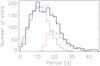 |
Fig. 8 Rotation period distribution of a subset of Kepler stars with Teff and log g similar to those of the Sun (namely, the RH⊙ sample). The original sample was obtained from Reinhold et al. (2013) combined with Huber et al. (2014). The symbols are the same as in Fig. 6. |
Figure 8 presents the rotation period distribution of a Sun-like subset of sources of Reinhold et al. (2013) combined with Huber et al. (2014), namely, the RH⊙ sample. This is a highly populated stellar set, similar to the MH⊙ sample, also selected within the elliptical region depicted in Fig. 1 (bottom panel) and within −0.2 dex < [Fe/H] < 0.2 dex. In addition, the detectability parameter of the RH⊙ sample, Rvar, can be easily simulated because its numerical value is highly similar to that of the variability amplitude A. Therefore, this sample allows for the most detailed and complete analysis of the Prot distribution in the present work.
The Prot distribution of the RH⊙ sample is noticeably different than that of the MH⊙ sample. One reason is certainly the different time spans of the LCs (the RH⊙ sample uses only Q3 data, the MH⊙ sample uses Q3-Q14 data), which facilitates long-period detection in the MH⊙ sample. Despite the difference, the distribution is also bimodal and can be decomposed into groups I and II, as performed for the samples analyzed above. In the synthetic sample, when groups I and II were initially decomposed by the regions below and above the 1 Gyr isochrone (giving ρI and ρII of 81% and 19%, respectively), the Prot distribution fit the observations reasonably well. However, the best fit was obtained by adjusting ρI and ρII to 72% and 28%, respectively. As suggested in Sect. 4, a normal distribution was defined for group I, which agreed with observations by peaking at approximately 11.3 ± 0.8 d with a standard deviation of approximately 5.4 ± 1.3 d. Hence, this distribution is compatible with the RH⊙ sample. Exponential decays also provided acceptable fits and produced similar behaviors, which did not improve the results.
For the entire Prot distribution of this sample, a noteworthy fit was obtained because the simulation was able to properly reproduce the bias caused by the detectability parameter Rvar. Indeed, we verified that for the RH⊙ sample, if S/N was used as the detectability parameter instead of A, a discrepancy would occur between the simulation and observations in the distribution decay around the solar period, similar to the problem of the MH⊙ sample. Therefore, an appropriate simulation of the detectability parameter certainly contributes to an optimal fit with observations. Because the synthetic distribution has the theoretical grid of Ekström et al. (2012) as a basic ingredient, which unbiasedly fit the Sun and Sun-like stars, the good fit indicates that the solar Prot is normal with regard to Sun-like stars.
Compared to the other CoRoT and Kepler samples, the period distribution of group I is compatible with the RH⊙ sample, and centered around a longer period and with a broader spread than in the DMS⊙ sample. This supports the possible relation of the group I distribution with the stellar population, as mentioned in Sect. 5.3. Indeed, the CoRoT fields lie toward the center and anti-center of the Galaxy, covering very many stars located near the Galactic plane. This region is expected to be more populated by young stars than at high Galactic latitudes (e.g., Miglio et al. 2013). The CoRoT fields are also small, covering together a region of ~8 sq. deg. In contrast, the Kepler field is considerably larger (~105 sq. deg) and covers a broad range of Galactic latitudes (Miglio et al. 2013; Girardi et al. 2015). These facts suggest a higher proportion and a narrower distribution of young stars in the CoRoT sample than in the Kepler sample. To test this hypothesis, we used the TRILEGAL code to obtain a sampling of the CoRoT and Kepler fields, covering nearly the same regions of their actual coordinates. The limiting magnitude was chosen to be V = 16 mag for the CoRoT fields and Kp = 17 mag for the Kepler field. Then we restricted the Teff, log g, and [M/H] (assumed to be ≃[Fe/H]) ranges according to our own selection of Sun-like stars. Based on this test, the age distribution of the CoRot and Kepler samples agrees well with the Prot distributions presented here, where the CoRoT fields include a greater proportion of young stars than older stars. In the Kepler field simulation, the simulation is much broader, with a considerably fewer young stars than in the CoRoT sample.
Despite this difference, either the CoRoT or Kepler fields comprise a high proportion of young objects. Overall, 64–84% of the Sun-like samples analyzed here are younger than ~1 Gyr. This result (restricted to Sun-like stars) is reasonable if compared with a related estimate from Matt et al. (2015), valid for the whole sample of Kepler sources, based on a relatively simple stellar rotation model. According to these authors, ~95% of the whole sample of Kepler field stars with Prot measurements are younger than ~4 Gyr.
In general, our study shows that the CoRoT and Kepler data can be well interpreted in terms of two populations, one young (group I), one older (group II), and with a different ratio between them. The proportions ρI and ρII for the CoRoT and Kepler samples considered here can be well interpreted by simulating the experiment sensitivity and biases. At least on the basis of the present data, there is no clear reason to believe that the bimodality reported by McQuillan et al. (2013a, 2014) can be explained by selection biases. As such, we support the suggestion of these authors, with some addition. The bimodality is possibly explained by a “natural bias” (i.e., not dependent on measurement sensitivity, but related to evolutionary duration) considering that two stellar populations experience evolutionary phases that have very different durations. These populations are, in fact, the groups I and II defined here. Therefore, the detectability bias is not the reason of the bimodality, although it influences the proportions ρI and ρII.
Of course, the normal distribution adopted here for group I is an approximation that may have a number of implicit biases. In contrast, the distribution of group II is based on a more elaborate set of theoretical models and assumptions, including the theoretical grids provided by Ekström et al. (2012), modeled parent distributions, the empirical period-amplitude relations by Messina et al. (2001, 2003), the selection by S/N, A, or w (which mimic detectability biases of the rotational modulation), and final filtering by Sun-like characteristics, all described in Sect. 3. Hence, the set of ingredients we presented allows us to study solar rotation by comparing actual and biased observations with theoretical models, within a precision that depends on the current data and model limitations. More refined studies can be developed in the future with this method. In particular, a potential improvement of the current results would be possible if spot-induced variability amplitudes were included in the stellar evolution codes with rotation.
6. Conclusions
We presented for the first time a quantified method with which the empirical distribution of Prot for Sun-like stars can be explained by considering the detectability of rotational modulation, which is related to the variability amplitude. The interpretations were based on a comparison between synthetic and empirical subsamples of CoRoT and Kepler field stars with physical parameters similar to those of the Sun.
For this purpose, we combined the public data of rotation periods with physical parameters for three stellar samples. The first sample was obtained from a CoRoT catalog with period measurements given by DM13, combined with spectroscopic physical parameters log g and Teff determined by Sarro et al. (2013), namely, the DMS sample. The selection of Sun-like stars was obtained within an elliptical region around the solar location in the HR diagram. For CoRoT stars, the subsample was enclosed by Teff = 5772 ± 300 K and log g = 4.44 ± 0.4 dex, namely, the DMS⊙ sample. The two other samples were selected from Kepler catalogs of rotation periods provided by Reinhold et al. (2013) and McQuillan et al. (2014), each combined with an improved compilation of physical parameters given by Huber et al. (2014). The Sun-like subsamples were selected within −0.2 dex < [Fe/H] < 0.2 dex and within an ellipsis described by Teff = 5772 ± 170 K and log g = 4.44 ± 0.2 dex, namely, the RH⊙ and MH⊙ samples.
To explain the observational biases, synthetic samples were generated based on the parent samples of the CoRoT and Kepler fields. The synthetic stars were separated into two groups, I and II, which are those located below and above the 1 Gyr isochrone in the HR diagram, respectively. These represent a group of young stars and a group composed of MS and evolved stars, respectively. For group I, synthetic rotation periods were randomly generated following two possible distributions compatible with PMS Sun-like stars: normal or an exponential decay from the peak. For group II, theoretical periods from Ekström et al. (2012) were set up according to the HR diagram location of the synthetic stars. Next, period-amplitude relations from Messina et al. (2001, 2003) were used to aggregate amplitude values to the synthetic samples, and random noise levels were added to these samples. Then, the main bias related to the detectability of the rotational modulation was applied to the synthetic stars by selecting them with a threshold in the variability S/N, A, or w (from McQuillan et al. 2014, which was particularly difficult to simulate) according to each observed sample. Finally, Sun-like subsamples were obtained by selecting the targets located within the ellipses described around the solar location in the HR diagram from the synthetic samples. The ellipses were defined within the same regions as for each one of the three observational subsamples of Sun-like stars considered here, namely, the DMS⊙, RH⊙, and MH⊙ samples.
The distribution in the HR diagram of the DMS sample has a large number of stars with low masses that are particularly similar to that of the Sun. This sample was obtained by identifying a well-defined semi-sinusoidal signature in the light curves without knowledge of their physical parameters, apart from photometric magnitudes and colors. This sample indicated that the semi-sinusoidal signature, defined by DM13, provides a good selection of low-mass spotted rotating stars, with a high occurrence for stars with masses of ~1 M⊙, which may have important implications in the relation between rotation and chromospheric activity for evolving Sun-like stars.
The rotation period distribution of the DMS⊙ sample is not clearly bimodal, but it fits our bimodal model, thus showing a high occurrence of young stars. The proportions of stars belonging to groups I and II with respect to the total number of objects in the synthetic sample, namely, ρI and ρII, are of 84% and 16%, respectively. These proportions fit the observations when simply separated by the 1 Gyr isochrone without any complementary adjustment. In addition, the full distribution of the synthetic sample, that is, the sum of groups I and II, exhibited a close fit with the observed distribution. This shows that separating the two groups by using the 1 Gyr isochrone is reasonable. Because of the relatively low number of objects in the DMS⊙ sample (175 targets), we cannot make conclusions regarding the solar rotation normality with respect to its Sun-like counterparts. Therefore, this result helps to validate the methods used to produce our biased synthetic samples. Further in-depth analyses can be performed from the Kepler data.
For the MH⊙ sample, the period distribution is more seemingly bimodal and has considerably more stars (2525 targets) than the DMS⊙ sample. For this case, the proportions ρI and ρII originally did not fit the observations well and was adjusted to final proportions of 64% and 36%, respectively. With this adjustment, the modeled distribution fit the observations well, although it exhibited a noticeable discrepancy in the distribution decay that traverses the solar rotation period. However, near the solar period, the synthetic sample fits the observations well, which suggests that the solar rotation period is normal with respect to Sun-like stars.
The period distribution of the RH⊙ sample also shows a bimodality and has a high number of stars (1836 targets), similar to the MH⊙ sample. The proportions ρI and ρII originally fit the observations well, although the best fit was obtained by adjusting these parameters to the final values of 72% and 28%, respectively. With this adjustment, the full period distribution of the synthetic sample provided an extremely close fit with observations. This fact strongly supports that the solar Prot is normal with respect to Sun-like stars.
Overall, the main conclusions of this work can be summarized as follows:
-
i.
The synthetic samples were able to explain the observedProt distributions by resolving them into two different populations, group I for young stars and group II for main-sequence and evolved stars, which generally produce a bimodal arrangement.
-
ii.
The central peak and the width of the group I Prot distribution may be related with the stellar population within a certain FOV.
-
iii.
Reasonable to optimal fits of the synthetic samples with the observed data were obtained especially by adjusting the bimodal peak levels with ρI and ρII and by refining the distribution slope at long periods with an appropriate detectability threshold for each Sun-like sample.
-
iv.
Several tests indicated that the parameters considered in these fits (see Table 1) provide a simple description of the Prot distributions without degeneracy.
-
v.
A detectability threshold is mandatory to properly fit synthetic with observed data for the CoRoT sample, while it improves the fits for the Kepler samples, but with a weaker effect. This suggests the Kepler samples are less biased by the variability amplitude than the CoRoT sample.
-
vi.
Best fits suggest a high number (64–84%) of young objects in the Sun-like samples, which explains the short Prot values of Sun-like stars on average compared to the solar value.
-
vii.
The global agreement between the synthetic and observed samples suggests the normality of the solar Prot, at least within the current data accuracy and model limitations.
Therefore, the method presented in this work allowed us to constrain observations on theory by considering biased samples with Prot measurements and was particularly useful to analyze field Sun-like stars. In addition, the following perspectives can improve our results:
-
i.
A substantial improvement of the synthetic samples will bepossible once stellar evolution models can predict thephotometric amplitude variations produced by rotating starspots. Such a theoretical prediction needs a description of themagnetic activity at the surface of stars, and the interpretation ofthe observed relation betweenProt and A is one of the observational facts that can help in this subject.
-
ii.
Observed data with more accurate physical parameters will provide a more refined selection of Sun-like stars and a more reliable separation of groups I and II. Accordingly, future spectroscopic observations, such as those to be collected with the Gaia-ESO Survey9 (Gilmore et al. 2012), will allow a better verification of our results.
The solar period ranges from 24.47 days at the equator to 33.5 days at the poles and has an avearage of 26.09 days (Lanza et al. 2003).
Semi-sinusoidal variability is characterized by some asymmetry of the maximum and minimum flux with respect to its average over time, somewhat irregular long-term amplitude variations, and semi-regular multi-sinusoidal short-term flux variations, typically with an amplitude ≲0.5 mag and period ≳0.3 days. This description is based on the dynamic behavior of star spots, as observed for the Sun (see DM13, Sect. 2.2).
Acknowledgments
This paper includes data collected by the Kepler mission. Funding for the Kepler mission is provided by the NASA Science Mission directorate. Research activities of the Observational Astronomy Stellar Board at the Federal University of Rio Grande do Norte are supported by continuous grants from the brazilian agencies CNPq and FAPERN and by the INCT-INEspaço. I.C.L. acknowledges post-doctoral PNPD/CNPq and post-doctoral PDE/CNPq fellowships. I.C.L. also thanks ESO/Garching for hospitality. C.E.F.L. acknowledges a post-doctoral PDJ/INCT-INEspaço/CNPq fellowship. L.P. acknowledges a distinguished visitor PVE/CNPq appointment at the DFTE/UFRN. L.P. also thanks DFTE/UFRN for hospitality and support of the INCT-INEspaço. V.N. acknowledges A BJT/CNPq fellowship. L.L.A.O. and D.F.S. acknowledge MSc fellowships of the CNPq. A.A.R.V. acknowledges support from FONDECYT postdoctoral grants #3140575, Ministry for the Economy, Development, and Tourism’s Programa Iniciativa Científica Milenio through grant IC 210009, awarded to the Millennium Institute of Astrophysics (MAS), CAPES grant PNPD/2011-Institucional, and the CNPq Brazilian agency. The authors thank the anonymous referee for very valuable comments and suggestions. We warmly thank F. Gallet for kindly providing us his catalog of rotation periods of PMS Sun-like stars, which was used in this work. The authors thank the CoRoT and Kepler staff for the development, operation, maintenance, and success of the mission. This work used the VizieR Catalogue Service operated at the CDS, Strasbourg, France.
References
- Affer, L., Micela, G., Favata, F., et al. 2012, MNRAS, 424, 11 [NASA ADS] [CrossRef] [Google Scholar]
- Affer, L., Micela, G., Favata, F., et al. 2013, MNRAS, 430, 1433 [NASA ADS] [CrossRef] [Google Scholar]
- Aigrain, S., Llama, J., Ceillier, T., et al. 2015, MNRAS, 450, 3211 [NASA ADS] [CrossRef] [Google Scholar]
- Baglin, A., Auvergne, M., Barge, P., et al. 2009, IAUS, 253, 71 [Google Scholar]
- Barnes, S. A. 2007, ApJ, 669, 1167 [NASA ADS] [CrossRef] [Google Scholar]
- Basri, G., Walkowicz, L. M., Batalha, N., et al. 2010, ApJ, 713, L155 [NASA ADS] [CrossRef] [Google Scholar]
- Basri, G., Walkowicz, L. M., Batalha, N., et al. 2011, AJ, 141, 20 [NASA ADS] [CrossRef] [Google Scholar]
- Bertone, E., Buzzoni, A., Chávez, M., & Rodríguez-Merino, L. H. 2008, A&A, 485, 823 [NASA ADS] [CrossRef] [EDP Sciences] [Google Scholar]
- Blomme, J., Debosscher, J., De Ridder, J., et al. 2010, ApJ, 713, L204 [Google Scholar]
- Brun, A. S., García, R. A., Houdek, G., et al. 2014, Space Sci. Rev., in press, DOI: 10.1007/s11214-014-0117-8 [Google Scholar]
- Charbonneau, P. 2010, Liv. Rev. Sol. Phys., 7, 3 [Google Scholar]
- Charbonneau, P. 2013, Nature, 493, 613 [NASA ADS] [CrossRef] [PubMed] [Google Scholar]
- Datson, J., Flynn, C., & Portinari, L. 2012, MNRAS, 426, 484 [NASA ADS] [CrossRef] [Google Scholar]
- Debosscher, J., Sarro, L. M., Aerts, C., et al. 2007, A&A, 475, 1159 [NASA ADS] [CrossRef] [EDP Sciences] [Google Scholar]
- Debosscher, J., Sarro, L. M., López, M., et al. 2009, A&A, 506, 519 [NASA ADS] [CrossRef] [EDP Sciences] [Google Scholar]
- Deheuvels, S., Dogan, G., Goupil, M. J., et al. 2014, A&A, 564, A27 [NASA ADS] [CrossRef] [EDP Sciences] [Google Scholar]
- de Freitas, D. B., Leão, I. C., Lopes, C. E. F., et al. 2013, ApJ, 773, L18 [NASA ADS] [CrossRef] [Google Scholar]
- De Medeiros, J. R., Lopes, C. E. F., Leão, I. C., et al. 2013, A&A, 555, A63 (DM13) [NASA ADS] [CrossRef] [EDP Sciences] [Google Scholar]
- Eggenberger, P., Meynet, G., Maeder, A., et al. 2008, Ap&SS, 316, 43 [NASA ADS] [CrossRef] [Google Scholar]
- Ekström, S., Georgy, C., Eggenberger, P., et al. 2012, A&A, 537, A146 [NASA ADS] [CrossRef] [EDP Sciences] [Google Scholar]
- Gallet, F., & Bouvier, J. 2013, A&A, 556, A36 [NASA ADS] [CrossRef] [EDP Sciences] [Google Scholar]
- García, R. A., Ceillier, T., Salabert, D., et al. 2014, A&A, 572, A34 [NASA ADS] [CrossRef] [EDP Sciences] [Google Scholar]
- Gazzano, J.-C., de Laverny, P., Deleuil, M., et al. 2010, A&A, 523, A91 [NASA ADS] [CrossRef] [EDP Sciences] [Google Scholar]
- Georgy, C., Granada, A., Ekström, S., et al. 2014, A&A, 566, A21 [NASA ADS] [CrossRef] [EDP Sciences] [Google Scholar]
- Giampapa, M. S. 2011, IAUS, 273, 68 [NASA ADS] [Google Scholar]
- Gilmore, G., Randich, S., Asplund, M., et al. 2012, The Messenger, 147, 25 [NASA ADS] [Google Scholar]
- Girardi, L., Groenewegen, M. A. T., Hatziminaoglou, E., et al. 2005, A&A, 436, 895 [NASA ADS] [CrossRef] [EDP Sciences] [Google Scholar]
- Girardi, Léo, Barbieri, M., Miglio, A., et al. 2015, in Asteroseismology of stellar populations in the Milky Way, Astrophys. Space Sci. Proc., 39, 125 [Google Scholar]
- Gonzalez, G. 1999, MNRAS, 308, 447 [NASA ADS] [CrossRef] [Google Scholar]
- Gonzalez, G. 2001, AJ, 121, 432 [NASA ADS] [CrossRef] [Google Scholar]
- Goupil, M. J., Mosser, B., Marques, J. P., et al. 2013, A&A, 549, A75 [NASA ADS] [CrossRef] [EDP Sciences] [Google Scholar]
- Gray, D. 1982, ApJ, 261, 259 [NASA ADS] [CrossRef] [Google Scholar]
- Gustafsson, B. 1998, Space Sci. Rev., 85, 419 [NASA ADS] [CrossRef] [Google Scholar]
- Habets, G. M. H. J., & Heintze, J. R. W. 1981, A&AS, 46, 193 [NASA ADS] [Google Scholar]
- Hartman, J. D., Bakos, G. A., Kovacs, G., et al. 2010, MNRAS, 408, 475 [NASA ADS] [CrossRef] [Google Scholar]
- Horne, J. H., & Baliunas, S. L. 1986, ApJ, 302, 757 [NASA ADS] [CrossRef] [Google Scholar]
- Hubeny, I., & Lanz, T. 1995, ApJ, 439, 875 [Google Scholar]
- Huber, D., Silva Aguirre, V., Matthews, J. M., et al. 2014, ApJS, 211, 2 [NASA ADS] [CrossRef] [Google Scholar]
- Jones, N. 2013, Nature, 493, 154 [NASA ADS] [CrossRef] [Google Scholar]
- Koch, D. G., Borucki, W. J., Basri, G., et al. 2010, ApJ, 713, L79 [NASA ADS] [CrossRef] [Google Scholar]
- Leão, I. C., de Laverny, P., Mékarnia, D., et al. 2006, A&A, 455, 187 [NASA ADS] [CrossRef] [EDP Sciences] [Google Scholar]
- Lanza, A. F., Rodonò, M., Pagano, I., et al. 2003, A&A, 403, 1135 [NASA ADS] [CrossRef] [EDP Sciences] [Google Scholar]
- Lucy, L. B. 1974, AJ, 79, 745 [NASA ADS] [CrossRef] [Google Scholar]
- Lomb, N. R. 1976, Ap&SS, 39, 447 [NASA ADS] [CrossRef] [Google Scholar]
- Mamajek, E. E., & Hillenbrand, L. A. 2008, ApJ, 687, 1264 [NASA ADS] [CrossRef] [Google Scholar]
- Maeder, A., & Meynet, G. 2015, IAU Symp., 307, 9 [Google Scholar]
- Matt, S. P., Brun, A. S., Baraffe, I., et al. 2015, ApJ, 799, L23 [NASA ADS] [CrossRef] [Google Scholar]
- McQuillan, A., Aigrain, S., & Mazeh, T. 2013a, MNRAS, 432, 1203 [NASA ADS] [CrossRef] [MathSciNet] [Google Scholar]
- McQuillan, A., Mazeh, T., & Aigrain, S. 2013b, ApJ, 775, L11 [NASA ADS] [CrossRef] [Google Scholar]
- McQuillan, A., Mazeh, T., & Aigrain, S. 2014, ApJS, 211, 24 [NASA ADS] [CrossRef] [MathSciNet] [Google Scholar]
- Meibom, S., Barnes, S. A., Latham, D. W., et al. 2011, ApJ, 733, L9 [NASA ADS] [CrossRef] [Google Scholar]
- Meléndez, J., Dodds-Eden, K., & Robles, J. A. 2006, ApJ, 641, 133 [NASA ADS] [CrossRef] [Google Scholar]
- Melott, A. L., & Thomas, B. C. 2011, Astrobiology, 11, 343 [NASA ADS] [CrossRef] [PubMed] [Google Scholar]
- Messina, S., Rodonò, M., & Guinan, E. F. 2001, A&A, 366, 215 [NASA ADS] [CrossRef] [EDP Sciences] [Google Scholar]
- Messina, S., Pizzolato, N., Guinan, E. F., et al. 2003, A&A, 410, 671 [NASA ADS] [CrossRef] [EDP Sciences] [Google Scholar]
- Metcalfe, T. S., Buccino, A. P., Brown, B. P., et al. 2013, ApJ, 763, L26 [NASA ADS] [CrossRef] [Google Scholar]
- Miglio, A., Chiappini, C., Morel, T., et al. 2013, MNRAS, 429, 423 [NASA ADS] [CrossRef] [Google Scholar]
- Nielsen, M. B., Gizon, L., Schunker, H., et al. 2013, A&A, 557, L10 [NASA ADS] [CrossRef] [EDP Sciences] [Google Scholar]
- Palacios, A. 2013 in Role and mechanisms of angular momentum transport during the formation and early evolution of stars, eds. P. Hennebelle, & C. Charbonnel, EAS PS, 62, 227 [Google Scholar]
- Porto de Mello, G. F., & da Silva, L. 1997, ApJ, 482, L89 [NASA ADS] [CrossRef] [Google Scholar]
- Prugniel, P., & Soubiran, C. 2001, A&A, 369, 1048 [NASA ADS] [CrossRef] [EDP Sciences] [Google Scholar]
- Prugniel, P., & Soubiran, C. 2004, Arxiv e-prints [arXiv:astro-ph/0409214] [Google Scholar]
- Reinhold, T., Reiners, A., & Basri, G. 2013, A&A, 560, A4 [NASA ADS] [CrossRef] [EDP Sciences] [Google Scholar]
- Richardson, W. H. 1972, J. Opt. Soc. Amer., 62, 55 [Google Scholar]
- Robles, J. A., Lineweaver, C. H., Grether, D., et al. 2008, ApJ, 684, 691 [NASA ADS] [CrossRef] [Google Scholar]
- Sarro, L. M., Debosscher, J., Neiner, C., et al. 2013, A&A, 550, A120 [NASA ADS] [CrossRef] [EDP Sciences] [Google Scholar]
- Scargle, J. D. 1982, ApJ, 263, 835 [NASA ADS] [CrossRef] [Google Scholar]
- Schuler, S. C., Cunha, K., Smith, V. V., et al. 2011, ApJ, 737, L32 [NASA ADS] [CrossRef] [Google Scholar]
- Shibata, K., Isobe, H., Hillier, A., et al. 2013, PASJ, 65, 49 [NASA ADS] [Google Scholar]
- Skumanich, A. 1972, ApJ, 171, 565 [NASA ADS] [CrossRef] [Google Scholar]
- Soderblom, D. 1983, ApJS, 53, 1 [NASA ADS] [CrossRef] [Google Scholar]
- Spada, F., Lanzafame, A. C., Lanza, A. F., et al. 2011, MNRAS, 416, 447 [NASA ADS] [Google Scholar]
- Steinhilber, F., & Beer, J. 2013, J. Geophys. Res. Space Phys., 118, 1861 [NASA ADS] [CrossRef] [Google Scholar]
- Strassmeier, K. G. 2009, A&ARv, 17, 251 [NASA ADS] [CrossRef] [Google Scholar]
- Strassmeier, K., Washuettl, A., Granzer, Th., et al. 2000, A&AS, 142, 275 [NASA ADS] [CrossRef] [EDP Sciences] [Google Scholar]
- Walkowicz, L. M., & Basri, G. S. 2013, MNRAS, 436, 1883 [NASA ADS] [CrossRef] [Google Scholar]
- Zahn, J.-P. 1992, A&A, 265, 115 [NASA ADS] [Google Scholar]
All Tables
All Figures
|
Fig. 1 Probability distribution in the HR diagram for the parent samples considered in this work. Top panel: distribution for the CoRoT field, obtained from the full sample of Sarro et al. (2013). Bottom panel: distribution for the Kepler field, computed from a subselection of Huber et al. (2014) with a metallicity −0.2 dex < [Fe/H] < 0.2 dex. The red–green–blue color gradient in the map represents decreasing probability; the high end is the red part of the gradient. Solid lines indicate the 1 Gyr isochrone of Ekström et al. (2012), and dashed lines illustrate the 1 M⊙ theoretical track provided by the same authors. The Sun is represented by its standard symbol. The ellipses around the solar location depict the subsamples of Sun-like stars (Sun-like samples). These were selected equally within the typical uncertainties in Teff and log g for each parent sample for observed and synthetic data (see text). |
| In the text | |
|
Fig. 2 Probability maps for the empirical magnitude-noise diagrams of the CoRoT (top panel) and Kepler (bottom panel) parent samples. |
| In the text | |
|
Fig. 3 Probability map for the empirical amplitude-weight diagram, A versus w, of the Kepler parent sample. Public w values were obtained from McQuillan et al. (2014), but we independently computed the A values. |
| In the text | |
|
Fig. 4 Rotation period distribution of the PMS Sun-like cluster stars selected by Gallet & Bouvier (2013). These stars belong to 13 star-forming regions or open clusters with ages ranging from 1 Myr to 1 Gyr and masses between 0.9 and 1.1 M⊙. The red dashed curve is a Gaussian fit with this distribution for periods greater than one day (see text). The blue dotted curve is an exponential fit with this distribution, where the origin of the exponential function was placed in the distribution peak (see text). |
| In the text | |
|
Fig. 5 Top panel: HR diagram for the CoRoT rotating candidates of DM13 combined with the physical parameters of Sarro et al. (2013), namely, the DMS sample. Circle sizes and colors represent the period intervals shown in the legend. Theoretical tracks from Ekström et al. (2012) are plotted as solid lines for different masses, identified by corresponding labels. The colors represent theoretical rotation periods within the same intervals as in the legend. The typical Teff and log g uncertainties are illustrated by the error bars. The Sun-like sample is denoted within the ellipsis around the solar location. Bottom panel: photometric period as a function of effective temperature for the same sample as the top panel. The red solid lines represent theoretical tracks from Ekström et al. (2012) for four different masses. The Sun is denoted in both panels by the solar symbol. |
| In the text | |
|
Fig. 6 Rotation period distribution of a subset of CoRoT stars with Teff and log g similar to those of the Sun (the DMS⊙ sample). The original sample was obtained from DM13 combined with Sarro et al. (2013; the DMS sample). The black histogram shows the actual distribution. The blue and red histograms and the dotted curve correspond to a modeled distribution of the actual data where biases were simulated. Blue depicts a group of young stars (group I), red depicts a group of MS and evolved stars (group II), and the dotted curve is the sum of these two group distributions. The latter, which is the full distribution, is the synthetic data considered to fit with observations. For illustrative purposes, the levels of the modeled distributions were adjusted to make the total number of synthetic stars similar to that of the actual sample. |
| In the text | |
|
Fig. 7 Rotation period distribution of a newer subset of Kepler stars with Teff and log g similar to those of the Sun (the MH⊙ sample). The original sample was obtained from McQuillan et al. (2014) combined with Huber et al. (2014). The symbols are the same as in Fig. 6. |
| In the text | |
|
Fig. 8 Rotation period distribution of a subset of Kepler stars with Teff and log g similar to those of the Sun (namely, the RH⊙ sample). The original sample was obtained from Reinhold et al. (2013) combined with Huber et al. (2014). The symbols are the same as in Fig. 6. |
| In the text | |
Current usage metrics show cumulative count of Article Views (full-text article views including HTML views, PDF and ePub downloads, according to the available data) and Abstracts Views on Vision4Press platform.
Data correspond to usage on the plateform after 2015. The current usage metrics is available 48-96 hours after online publication and is updated daily on week days.
Initial download of the metrics may take a while.