| Issue |
A&A
Volume 582, October 2015
|
|
|---|---|---|
| Article Number | A111 | |
| Number of page(s) | 7 | |
| Section | Cosmology (including clusters of galaxies) | |
| DOI | https://doi.org/10.1051/0004-6361/201525736 | |
| Published online | 20 October 2015 | |
Testing the homogeneity of the Universe using gamma-ray bursts⋆
1
Institute of Astronomy and Space Science, Sun Yat-Sen
University,
510275
Guangzhou,
PR China
e-mail: This email address is being protected from spambots. You need JavaScript enabled to view it.
; This email address is being protected from spambots. You need JavaScript enabled to view it.
2
Department of Physics, Chongqing University,
401331
Chongqing, PR
China
Received: 26 January 2015
Accepted: 29 July 2015
Abstract
Aims. The discovery of a statistically significant clustering in the distribution of gamma-ray bursts (GRBs) has recently been reported. Given that the cluster has a characteristic size of 2000–3000 Mpc and a redshift between 1.6 ≤ z ≤ 2.1, it has been claimed that this structure is incompatible with the cosmological principle of homogeneity and isotropy of our Universe. In this paper, we study the homogeneity of the GRB distribution using a subsample of the Greiner GRB catalogue, which contains 314 objects with redshift 0 < z < 2.5 (244 of them discovered by the Swift GRB mission). We try to reconcile the dilemma between the new observations and the current theory of structure formation and growth.
Methods. To test the results against the possible biases in redshift determination and the incompleteness of the Greiner sample, we also apply our analysis to the 244 GRBs discovered by Swift and the subsample presented by the Swift Gamma-Ray Burst Host Galaxy Legacy Survey (SHOALS). The real space two-point correlation function (2PCF) of GRBs, ξ(r), is calculated using a Landy-Szalay estimator. We perform a standard least-χ2 fit to the measured 2PCFs of GRBs. We use the best-fit 2PCF to deduce a recently defined homogeneity scale. The homogeneity scale, RH, is defined as the comoving radius of the sphere inside which the number of GRBs N(<r) is proportional to r3 within 1%, or equivalently above which the correlation dimension of the sample D2 is within 1% of D2 = 3.
Results. For a flat ΛCDM Universe, a best-fit power law, ξ(r) = (r/r0)− γ, with the correlation length r0 = 413.64 ± 135.40 h-1 Mpc and slope γ = 1.57 ± 0.63 (at 1σ confidence level) for the real-space correlation function ξ(r) is obtained. We obtain a homogeneous distribution of GRBs with correlation dimension above D2 = 2.97 on scales of r ≥ 8200 h-1 Mpc. For the Swift subsample of 244 GRBs, the correlation length and slope are r0 = 387.51 ± 132.75 h-1 Mpc and γ = 1.57 ± 0.65 (at 1σ confidence level). The corresponding scale for a homogeneous distribution of GRBs is r ≥ 7700 h-1 Mpc. For the 75 SHOALS GRBs, the results are are r0 = 288.13 ± 192.85 h-1 Mpc and γ = 1.27 ± 0.54 (at 1σ confidence level), with the homogeneity scale r ≥ 8300 h-1 Mpc. For the 113 SHOALS GRBs at 0 < z < 6.3, the results are r0 = 489.66 ± 260.90 h-1 Mpc and γ = 1.67 ± 1.07 (at 1σ confidence level), with the homogeneity scale r ≥ 8700 h-1 Mpc.
Conclusions. The results help to alleviate the tension between the new discovery of the excess clustering of GRBs and the cosmological principle of large-scale homogeneity. It implies that very massive structures in the relatively local Universe do not necessarily violate the cosmological principle and could conceivably be present.
Key words: gamma rays: general / methods: data analysis / methods: statistical / large-scale structure of Universe / cosmology: observations / distance scale
Tables 1 and 2 are only available at the CDS via anonymous ftp to cdsarc.u-strasbg.fr (130.79.128.5) or via http://cdsarc.u-strasbg.fr/viz-bin/qcat?J/A+A/582/A111
© ESO, 2015
 Open Access article, published by EDP Sciences, under the terms of the Creative Commons Attribution License (http://creativecommons.org/licenses/by/4.0), which permits unrestricted use, distribution, and reproduction in any medium, provided the original work is properly cited.
1. Introduction
Gamma-ray bursts (GRBs) are the most energetic events in our Universe. Their cosmological origin has been studied by Klebesadel et al. (1973), Meegan et al. (1992), Kouveliotou et al. (1993), Costa et al. (1997), Paradijs et al. (1997), Harrison et al. (1999), Meszaros & Gehrels (2012). GRBs and luminous red galaxies (LRGs) are both luminous tracers of matter in our Universe. Unlike most LRGs, GRBs have a larger redshift range that reaches up to z ~ 8. They have minimum separations over 100 Mpc. Therefore, they are valid indicators of potential large-scale structures in the intermediate-redshift Universe.
According to modern cosmology, structures on different length scales in our Universe all have their origins in the quantum fluctuations of the inflation field, the scalar field which generates the inflation after the birth of our Universe. These primordial Gaussian random phase fluctuations, which later lead to the density fluctuations in different modes, enter the horizon on different epochs and grow as time passes by. This gives rise to the hierarchical scenario of the matter clustering – the fluctuations with longer comoving wavelengths enter the horizon later and have less time to evolve than the small-scale fluctuations. As large-scale structures are closely related to these long-wavelength modes, one can conclude that a finite age of our Universe would result in a limited maximum size of the large-scale structure in our Universe. Translated into the language of modern cosmology, it is the cosmological principle – the matter distribution in our Universe is homogeneous and isotropic on sufficiently large scales. On small scales, our Universe is inhomogeneous, with structures like galaxies and galaxies clusters.
The transition scale between homogeneity and inhomogeneity is called the “homogeneity scale”1. The homogeneity scale of the distribution of matter has long been studied and the results are quite scattered. Hogg et al. (2005) analysed the enormous LRG sample of the Sloan Digital Sky Survey (SDSS; York et al. 2000) and presented a homogeneity scale RH ~ 70h-1 Mpc. Similar results were obtained by Sarkar et al. (2009) and Scrimgeour et al. (2012), who performed a multifractal analysis over 200 000 blue luminous galaxies in the WiggleZ survey (Drinkwater et al. 2010). Sylos Labini et al. (2009) claimed to find a homogeneity scale above 100 h-1 Mpc after studying the galaxy catalogue of SDSS.
Horvath et al. (2014) have recently reported the discovery of a statistically significant clustering in the GRB sample between 1.6 ≤ z ≤ 2.1. They called it the Hercules-Corona Borealis Great Wall (Her-CrB GW). It has a characteristic scale of ~2000 Mpc and its longest dimension ~3000 Mpc, is six times larger than the size of the Sloan Great Wall. Its characteristic size is far above the upper limit of the homogeneity scale placed by the fractal dimensional analysis based on the galaxy surveys. The two-dimensional Kolmogorov-Smirnov test (Lopes et al. 2008) shows a 3σ deviation. The clustering excess cannot be entirely attributed to the known sampling biases. The existence of the potential structure, defined by the GRBs, is considered to be inconsistent with the cosmological principle and beyond the standard excursion set theory for structure growth.
In this paper, we examine the spatial distribution of the GRBs using a subsample of Greiner’s GRB catalogue, which contains 314 objects with redshift 0 < z < 2.5 (244 of them discovered by the Swift GRB mission). The sample encompasses the redshift region of the reported potential structure mapped by the GRBs. We first use the Landy-Szalay estimator (Landy & Szalay 1993) to estimate the real space two-point correlation function (2PCF) ξ(r) of the GRB sample. We fit a simple power law to the measured GRB ξ(r). We then use the best-fit ξ(r) to deduce the correlation dimension D2(r) and the homogeneity scale RH of the GRB distribution. To test the results against the possible biases in redshift determination and the incompleteness of the Greiner sample, we also apply the analysis to the subsample presented by the Swift Gamma-Ray Burst Host Galaxy Legacy Survey (SHOALS) in Perley et al. (2015). The results are plotted in the same figure for comparison.
The rest of the paper is organized as follows. In Sect. 2, we introduce the GRB sample and the techniques used in our analysis. The real-space 2PCF ξ(r) of the GRB sample and its best-fit power law are both obtained in this section. In Sect. 3, the definitions and calculations of homogeneity scale and correlation dimension are presented. We deduce the specific RH for the GRBs with 0 < z < 2.5. Relevant physical implications and comparisons to the results of other surveys are presented in Sect. 4.
2. Data and techniques
2.1. GRB catalogue and the subsample
In this work we primarily use a sample of 314 GRBs with redshift 0 < z < 2.5. All of these GRBs are from the collection presented by Greiner (2014)2; 244 of them come from the NASA Swift mission; and the rest come from BeppoSAX GRBM, HETE2, IPN, and INTEGRAL, etc. We use the data released on July 8, 2015. The entire sample contains more than 1000 objects. Only 431 of them have well-measured redshifts. The well-measured subsample has a redshift 0 < z < 9.2. In the redshift region z > 7, there are only two GRBs: GRB 090423 (z = 8.26) and GRB 090429B (z = 9.2). They are omitted from our numerical analysis since they are of little statistical significance. This leaves a subsample of 429 GRBs at 0 < z < 6.7. Given that the potential GRB structure reported by Horvath et al. (2014) has a redshift 1.6 < z < 2.1, we cut this sample down further by using only those GRBs having well-determined redshifts at 0 < z < 2.5, which encompasses the redshift region of the potential structure. We have a final subsample of 314 GRBs at redshift 0 < z < 2.5.
The redshifts of GRBs can be estimated in a number of ways, i.e. through the absorption spectroscopy of the optical afterglow (the vast majority of the Swift sample are measured in this way) or measuring the emission lines of their host galaxies (which is observationally expensive). Faintness of the afterglows of some events have left the sample intrinsically optically biased. Alternative approaches have been proposed to solve this problem (Kruhler et al. 2011; Rossi et al. 2012; Perley et al. 2013; Hunt et al. 2014). One of them is to develop a series of observability cuts with a set of optimized parameters to isolate a subset of the GRB sample (Jakobsson et al. 2006; Cenko et al. 2006; Perley et al. 2009; Greiner et al. 2011). Using this method, one can obtain a GRB sample whose afterglow redshift completeness is close to about 90% (Hjorth et al. 2012; Jakobsson et al. 2012; Kruhler et al. 2012; Salvaterra et al. 2012; Schulze et al. 2015), the level that is necessary for systematic biases not to dominate the statistical ones (Perley et al. 2015). Using this technique, Perley et al. (2015) established the largest and most complete (92% completeness) GRB redshift sample to date, which is called the SHOALS sample. The SHOALS sample contains 119 objects in total, 112 of which have well-determined redshifts at 0 < z < 6.3 (75 are at 0 < z < 2.5). To test the results against the possible biases in redshift determination and the incompleteness of the Greiner sample, we also apply our analysis to this subsample of GRBs.
Thus, we base our analysis primarily on the Greiner sample of 314 GRBs. In comparison, we also apply our analysis to the Swift subsample of 244 GRBs and the SHOALS very complete GRB sample. The angular and redshift distributions of these samples are plotted in Figs. 1a and b. The corresponding celestial coordinates and the redshifts of the objects in the Greiner sample and the SHOALS sample are listed respectively in Tables 1 and 2, which are available at the CDS. Most of them have a comoving separation r > 100 h-1 Mpc, with the longest separation distance up to r ~ 10 h-1 Gpc.
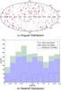 |
Fig. 1 Angular and redshift distributions of the GRB samples. a) The angular distribution of the GRB samples in J.2000 equatorial coordinates. The red solid dots represent the 244 GRBs at 0 < z < 2.5 detected by Swift, while the black solid dots represent those discovered by other detectors within the same redshift range. The red and black solid dots constitute Greiner’s GRB sample of 314 objects at 0 < z < 2.5. The blue circles represent the 112 GRBs (at 0 < z < 6.3) from SHOALS. b) The redshift distribution of the GRB data. The y-axis denotes the number of objects in each redshift bin. The green shaded area plus the purple area indicates the total of 314 GRBs from the Greiner sample. The dashed line represents the contribution from the SHOALS subsample of 75 objects at 0 < z < 2.5. |
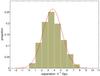 |
Fig. 2 Distribution of the comoving separations d between the GRBs in the Greiner sample (including the Swift subsample of 244 GRBs and most of the SHOALS GRBs). The x-axis is the comoving separation of the GRB data, in units of h-1 Gpc. The y-axis is the proportion of the GRB number in each bin to the whole sample, which has been normalized to 1. The separation d obeys a Gaussian distribution with the expectation value |

2.2. Two-point correlation function
Given a GRB in the spatial volume dV1, the 2PCF of GRBs, ξ(r), is defined as the probability of finding another GRB in dV2 with a separation distance r, i.e. (Peebles 1980) ![Mathematical equation: \begin{eqnarray} {\rm d}P_{12}={\bar n}^2[1+\xi(r)]{\rm d}V_1{\rm d}V_2, \end{eqnarray}](/articles/aa/full_html/2015/10/aa25736-15/aa25736-15-eq49.png) (1)where
(1)where  is the mean number density of the GRBs. To calculate ξ(r), an auxiliary random sample of NR points is generated in a window W of observations. A window W is a three-dimensional space of volume V, the same volume as that on which the observation was made.
A statistical estimation of ξ(r) involves a pair count of neighbouring GRBs at a given separation scale. The most widely used estimator of the 2PCF is the Landy-Szalay estimator  (Landy & Szalay 1993),
 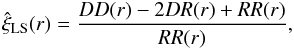 (2)where DD(r) and RR(r) are, respectively, the number of GRB pairs within the separation d ∈ [r − Δr/2,r + Δr/2] (Δr is the bin width used in the statistical estimation of ξ(r)) in the observed data set D and in the auxiliary random sample R in the window W, while DR(r) is the number of GRB pairs between the observed data and the random sample with the same separation. The parameter d is the comoving separation distance of GRBs. Specifically, DR(r) is defined as DR(r) ≡ NDR(r)/(NDNR) (ND and NR are, respectively, the total number of GRBs in the data set D and in the random sample R), where NDR(r) is given by (Kerscher et al. 2000)
 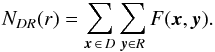 (3)The summation runs over all the coordinates of GRBs (represented by x and y) in the observed data set D and the random sample R in the window W. The value of the function F(x,y) equals 1 when the separation of the two objects is within the distance d(x,y) ∈ [r − Δr/2,r + Δr/2] or otherwise equals 0. The expressions DD(r) ≡ NDD(r)/[ND(ND − 1)] and RR(r) ≡ NRR(r)/[NR(NR − 1)] respectively represent the normalized number of GRB pairs within the separation mentioned above in the observed data set D and in the random sample R; NDD(r) and NRR(r) are defined in a similar way as NDR(r) in Eq. (3).
We use the jackknife resampling method to determine the statistical uncertainty of the measured 2PCF of GRBs. The jackknife method is an internal method of error estimation that is extensively used to determine the errors of 2PCF of galaxies and quasars (Ross et al. 2007; Sawangwit et al. 2011; Nikoloudakis et al. 2013). The entire sample is divided into N′ subsamples of roughly equal size. The jackknife error estimator is given as ![Mathematical equation: \begin{eqnarray} \sigma^2_{{\rm Jack}}(r)=\sum_{i^\prime\, =\,1}^{N^\prime}\frac{DR_{i^\prime} (r)}{DR(r)}[\xi_{i^\prime} (r)-\xi(r)]^2, \label{jackknife} \end{eqnarray}](/articles/aa/full_html/2015/10/aa25736-15/aa25736-15-eq76.png) (4)where ξi′(r) denotes the estimate of the 2PCF on all of the (N′ − 1) subsamples except the ith one.
(4)where ξi′(r) denotes the estimate of the 2PCF on all of the (N′ − 1) subsamples except the ith one.
2.3. Calculating the two-point correlation function, ξ(r)
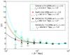 |
Fig. 3 Best-fit power law of the measured real-space 2PCF ξ(r) at 200 h-1<r < 104h-1 Mpc. We assume a flat ΛCDM cosmological model, with ΩΛ = 0.72, Ωm = 0.28, H0 = 100 h km s-1 Mpc-1, h = 0.7. The real-space 2PCF ξ(r) measured via Eq. (2) for the Greiner, Swift, and SHOALS samples are, respectively, indicated by green circles, red solid triangles, black solid diamonds, and cyan squares with 1σ jackknife error bars that are estimated from (4). The density of random points we use for the estimation is 20 times the density of GRB data. ξ(r) is plotted in equally spaced logarithmic intervals of Δlog 10(r) = 0.2 h-1 Mpc. The best-fit power laws of the form (5) for the measured ξ(r) are plotted in solid lines, with the best-fit parameters given in the legends. |
The estimation of the 2PCF of GRBs, ξ(r), is made by counting the pairs in and between the observed GRB distribution and a catalogue of randomly distributed GRBs. The density of random points that we use for the estimation is 20 times the density of the GRB data. We use a bin width of Δlog 10(r) = 0.2 h-1 Mpc. The estimation of ξ(r) depends on the assumed cosmology. We use a flat ΛCDM cosmological model (cold dark matter plus a cosmological constant Λ) in this work, with ΩΛ = 0.72, Ωm = 0.28, H0 = 100 h km s-1 Mpc-1, h = 0.7.
Furthermore, the 2PCF is usually measured in redshift space. As shown in Fig. 2, the GRBs in the observed sample have an average separation distance over 100h-1 Mpc (with the largest separation up to ~10 h-1 Gpc). On such a scale, the current structure formation theory predicts that the evolution and clustering of matter should still be in the linear regime at the present time (Springel et al. 2005; Eisenstein et al. 2007). The redshift-space distortions3 due to the small-scale peculiar velocities of the objects and the redshift variances are also minimal on this scale (Ross et al. 2007). Thus, the difference between the redshift-space and the real-space correlation functions on such large scales could be negligible. For convenience, the calculation and analysis in this paper are done in real space.
For the estimation of the jackknife error  , we take N′ = 5, and split the sample into five redshift regions with equal redshift intervals Δz = 0.5. The real-space 2PCFs in a flat ΛCDM Universe for Greiner’s 314 GRBs, the subsample of 244 objects discovered by Swift, and the SHOALS subsample are respectively plotted in Fig. 3 in equally spaced logarithmic intervals. It spans a comoving distance of scale 102h-1<r < 104h-1 Mpc.
A power law of the form 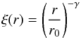 (5)is usually fitted to the correlation functions of galaxies and galaxy clusters (Davis & Peebles 1983; Bahcall 1988; Maddox et al. 1990; Peacock & West 1992; Dalton et al. 1994; Zehavi et al. 2004). The parameter r0 is the comoving correlation length, in units of h-1 Mpc. The slope γ is a dimensionless constant. Similarly, we fit a power law of the form in Eq. (5) to the measured 2PCF data over the range 200 h-1 ≤ r ≤ 104h-1 Mpc. We perform a standard least-χ2 fit. For a flat ΛCDM Universe, the best-fit values of the correlation length r0 and slope γ for the real-space correlation function ξ(r) for Greiner’s 314 GRB data at z < 2.5 are (with 1σ confidence level errors)
 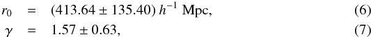 with
with  . For the subsample of 244 objects discovered by Swift, we obtain (with 1σ confidence level errors)
 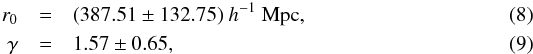 with
with  .
.
For the SHOALS subsample of 75 GRBs, the results are  with
with  . For the SHOALS sample of 113 GRBs at 0 < z < 6.3, the results are
  with
with  . From these results, one can see that the best-fit values of r0 and γ increase with the growing number of GRB data points as well as higher redshifts. We plot the best-fit power-law models of ξ(r) in Fig. 3.
3. Homogeneity of the GRB distribution
Given the best-fit 2PCF, ξ(r), for the GRB sample in the previous section, we are now in a position to calculate the homogeneity scale, RH, for the GRB distribution at 0 < z < 2.5. We first give a brief introduction of the correlation dimension D2(r) for a random distribution of data points. We describe the relation between the value of D2(r) and the concept of a homogeneous distribution. A more formal treatment of this section can be found in Yadav et al. (2010) and Scrimgeour et al. (2012).
3.1. Correlation dimension, D2(r)
Several methods have been developed to investigate the homogeneity of the galaxy distribution. The most popular among them is fractal analysis (Yadav et al. 2005). A fractal is a kind of geometrical object where every small part of it appears as a reduction of the entirety. In fractal analysis, the concept “fractal dimension” is invoked to describe the homogeneity of the distribution of a point set. One of the most common definitions of fractal dimension is the “correlation dimension”, D2(r). Unlike other homogeneity indicators, deviations caused by a size-limited sample would only result in second-order changes to D2(r). Thus, D2(r) is regarded as a robust measure of homogeneity and is extensively used in the homogeneity investigations of galaxies and quasars (Sylos Labini et al. 2009; Scrimgeour et al. 2012; Nadathur 2013).
In this paper, we use the working definition of D2(r) given in Scrimgeour et al. (2012) to study the homogeneity of the GRB distribution. We limit our discussions to a three-dimensional space. Given a set of points in space, the measurement of D2(r) is to find the average number of neighbouring points, N(<r) inside a three-dimensional sphere of radius r centered at each point. One can formulate the scaling behaviour of N(<r) as  (14)where D is the fractal dimension of the distribution. N(<r) can actually be given as
  , where is the mean number density of points in that region. For a homogeneous distribution of the point set, is a universal constant and N(<r) then scales as ∝r3. From Eq. (14), this implies D = 3. An inhomogeneous distribution would result in a non-universal . From Eq. (14), this gives D < 3 or D > 3: D < 3 stands for an inhomogeneous distribution of the point set, while D > 3 represents a “super-homogeneous” distribution (Gabrielli et al. 2002). In the literature, N(<r) is usually divided by the number expected for a homogeneous distribution,
  (here is a universal constant), to correct for incompleteness. The corrected N(<r) is given as
  (15)For a homogeneous distribution, one has
  .
.
In general, the correlation dimension D in Eq. (14) is a function of the sphere radius, r, i.e. D = D2(r). It can be deduced from the count-in-sphere number N(<r) as  (16)The correlation dimension D2(r) measures the scaling properties of
  without being affected by the amplitude of (which is related to the mean number density of the data points in the regions). It is therefore an objective measure of the homogeneity in the statistical analysis of matter distribution. To deduce the correlation dimension D2(r) for the GRB distribution, one should first calculate . For the GRBs can actually be obtained by integrating the 2PCF ξ(r) for the GRBs (Peebles 1980):
 ![Mathematical equation: \begin{eqnarray} {\mathcal N}({<}r)=\frac{3}{4\pi r^3}\int_0^r [1+\xi_{}(r^\prime)]4\pi r^{\prime 2}{\rm d}r^\prime. \label{Nfromxi} \end{eqnarray}](/articles/aa/full_html/2015/10/aa25736-15/aa25736-15-eq122.png) (17)Combining Eqs. (16) with (17), we obtain an analytical expression of D2(r):
(17)Combining Eqs. (16) with (17), we obtain an analytical expression of D2(r): ![Mathematical equation: \begin{eqnarray} D_2(r)=\frac{{\rm d}}{{\rm d}\!\ln r}\left\{ \ln\left[\frac{3}{4\pi r^3}\int_0^r [1+\xi_{}(r^\prime)]4\pi r^{\prime 2}{\rm d}r^\prime \right]\right\}+3. \label{D2v2} \end{eqnarray}](/articles/aa/full_html/2015/10/aa25736-15/aa25736-15-eq123.png) (18)Given the best-fit power law of ξ(r) as in Eq. (5) with the correlation length r0 and slope γ of ξ(r′) given in Eqs. (6) to (13), we are now in a position to estimate the homogeneity scale of the GRB distribution.
(18)Given the best-fit power law of ξ(r) as in Eq. (5) with the correlation length r0 and slope γ of ξ(r′) given in Eqs. (6) to (13), we are now in a position to estimate the homogeneity scale of the GRB distribution.
3.2. Scale of homogeneity, RH
There are several ways to define the homogeneity scale RH with respect to the correlation dimension D2(r). Yadav et al. (2010) defined the homogeneity scale as the scale above which the deviation of the fractal dimension D2(r) from the ambient spatial dimension becomes smaller than the statistical dispersion of D2(r) itself. For the limited size of the GRB sample that we use in our work, the statistical dispersion of D2(r) might be large. This effect of a limited sized sample would therefore enlarge the estimation of RH for our GRB sample. Following Scrimgeour et al. (2012), in our analysis we use a more robust definition of RH that is not affected by the sample size. Given the correlation dimension D2(r) of the GRB distribution, the homogeneity scale RH is defined as the scale on which D2(r) of the sample is within 1% of D2 = 3, i.e. D2(r = RH) = 2.97. An equivalent definition of RH can also be given by  , for which RH is defined as the comoving radius r of the sphere inside which the number of LQGs N(<r) is proportional to r3 within 1%, i.e.
  .
.
Using these definitions, we calculate the homogeneity scale of the distribution of the GRB sample. The theoretical prediction of D2(r) and the corresponding value of RH for the GRB samples are plotted in Fig. 4 for comparison. For Greiner’s sample of 314 GRBs, the homogeneity scale for the GRB distribution is RH ≃ 8200 h-1 Mpc, which means that the cosmological principle is retained on such a scale (r>RH). One should observe a homogeneous distribution of GRBs on scales r>RH. For the subsample of 244 GRBs discovered by Swift, the result is RH ≃ 7700 h-1 Mpc. For the SHOALS subsample of 75 GRBs at 0 < z < 2.5, we have RH = 8300 h-1 Mpc. For the SHOALS subsample of 113 GRBs at 0 < z < 6.3, we have RH = 8700 h-1 Mpc.
The scale of homogeneity RH for the GRBs can also be considered as the upper limit of the characteristic size of any clustering and structures in the GRB distribution. The potential structure mapped by the GRBs at 1.6 < z < 2.1 reported by Horvath et al. (2014) has a characteristic size of ~2000 Mpc and is thus well within the limits we obtain. Therefore, we conclude that the existence of such an excess clustering in the GRB distribution is still compatible with the cosmological principle and the standard theory of structure formation.
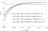 |
Fig. 4 Correlation dimension, D2(r), for different GRB samples. The D2(r) calculated from Eq. (18) is shown in solid lines. The dashed line indicates the critical value defined for the transition from a homogeneous to an inhomogeneous distribution of the GRBs, i.e. 1% from the homogeneity, D2(r) = 2.97. |
4. Conclusions and discussion
Redshift surveys (Drinkwater et al. 2010; Ahn et al. 2014) provide about a hundred thousand galaxies that can be used for a homogeneity investigation of the matter distribution in our Universe. Most of these galaxies have redshifts z < 1. GRBs usually have a larger redshift range than the galaxies (which can reaches up to z ~ 8) and thus provide valid luminous indicators of matter distribution in the intermediate-redshift universe. Quasars have redshifts as high as GRBs, but their observations only cover a limited sky area4. This involves specific technical treatment in data process when using the Landy-Szalay estimator to estimate the 2PCF for quasars (Karagiannis et al. 2014). Compared with galaxies and quasars, the GRB sample has a full-sky angular distribution and a redshift range up to z ~ 8. In fact, in our study we found that most GRBs have a comoving separation >100 h-1 Mpc (see Fig. 2) and therefore they provided an efficient probe of matter correlation on large scales in the intermediate-redshift universe. By “efficient” here, we mean that the size of the data we used to estimate ξ(r) on such a scale is much less than that used by galaxy or quasar surveys, since the number density of galaxies and quasars observed is much higher than GRBs. Using galaxies or quasars to probe the correlation and clustering on such a scale (e.g. r ~ 200 h-1 Mpc) would involve counting many more objects inside the sphere of radius r and therefore would cost more computing machine time than using GRBs.
In this paper we used a sample of 314 GRBs from the collection presented by Greiner (2014) to study the homogeneity of matter distribution on large scales. They cover a redshift range 0 < z < 2.5, 244 of which discovered by the Swift GRB mission. We calculated the real-space 2PCF, ξ(r), for GRBs on scales 102h-1<z < 104h-1 Mpc. The measured ξ(r) for GRBs on scales r > 200 h-1 Mpc can be well fitted by a power law of the form ξ(r) = (r/r0)− γ, with correlation length r0 = (413.64 ± 135.40) h-1 Mpc and slope γ = 1.57 ± 0.63 (1σ confidence level), and . For the subsample of 244 objects discovered by Swift, we obtained r0 = (387.51 ± 132.75) h-1 Mpc and γ = 1.57 ± 0.65 (1σ confidence level), with .
We then used the best-fit ξ(r) to deduce the homogeneity scale RH for the GRB distribution at 0 < z < 2.5. We obtained RH ≃ 8200 h-1 Mpc. For the subsample of 244 objects discovered by Swift, we obtained RH ≃ 7700 h-1 Mpc, which means that above such a scale GRBs can be considered to have a homogeneous distribution. On scales r <RH, an inhomogeneous distribution of GRBs is assumed for the standard excursion set theory of structure growth. The potential GRB structure recently reported by Horvath et al. (2014) has a characteristic size of ~2000 Mpc with its longest dimension ~3000 Mpc. Both are well below the homogeneity scale RH we deduced for the GRB distribution. This implies that the discovery of such an angular excess of the GRB distribution is still compatible with the cosmological principle, which assumes that the matter distribution of our Universe is homogeneous and isotropic over a large smoothing scale. For the distribution of GRBs, we suggested that such a scale is RH ≃ 8200 h-1 Mpc (which corresponds to RH ≃ 11.7 Gpc given the choice of h = 0.7). The comoving cosmic horizon5 within which causality holds are lH ≃ 10 Gpc at z ≃ 2 (the redshift of the potential GRB structure). The RH we obtained for the GRB distribution is slightly larger than the lH at z ≃ 2. We hope that with the growing size of the observed GRB sample and a more accurate measurement of the 2PCF ξ(r) of GRBs, this difference will be eliminated by future observations and investigations.
To test the results against the possible biases in redshift determination and the incompleteness of the Greiner sample, we also applied our analysis to the GRB subsample presented by SHOALS in Perley et al. (2015). Despite its limited sample size (with a total of 119 objects), the afterglow redshift completeness of the SHOALS GRB sample is 92%. It was proposed in order to strike a balance between redshift completeness and overall statistical size; the SHOALS GRB sample provides largest and most complete GRB redshift sample for clustering analysis to date. It has been employed to test the viability of our results against the biases and incompleteness of the Swift and Greiner samples. We obtained r0 = 288.13 ± 192.85 h-1 Mpc and γ = 1.27 ± 0.54 (at 1σ C.L.), with for the SHOALS 75 GRBs at 0 < z < 2.5. The deduced homogeneity scale is RH = 8300 h-1 Mpc. For the 113 objects in the SHOALS sample that have well-determined redshifts at 0 < z < 6.3, we obtained r0 = 489.66 ± 260.90 h-1 Mpc and γ = 1.67 ± 1.07 (at 1σ C.L.), with . The deduced homogeneity scale is RH = 8700 h-1 Mpc. Two comments are necessary. First, the best-fit values of r0 and γ increase with growing number of GRB data points as well as higher redshifts. This manifests itself in the results obtained from SHOALS’s GRB sample, and also in the results obtained from the Greiner sample. Second, one can see that the RH obtained from the SHOALS very complete GRB sample do not differ much from those obtained from the Greiner and Swift subsets, which implies that the Greiner GRB sample and the Swift GRB sample are both robust in the statistical analysis of clustering and matter distribution.
It should also be noted that for distributions of different objects, the scale of homogeneity RH are different because the different objects have different origins and evolution dynamics, and thus have different bias factors. The 2PCF can also be given by ξ(r) ≡ b2ξmass(r), where b is the bias factor for specific kinds of objects. Given the same 2PCF ξmass(r) of the underlying (dark) matter6, the amplitude of ξ(r) depends on the value of b. In general, b is a function of comoving radius r and redshift z, i.e. b = b(r,z). Thus, for different kinds of objects with different characteristic (mass) scales and redshifts, b(r,z) take different values, which would result in a varying amplitude of ξ(r). From Eq. (18), one can expect a different homogeneity scale RH for the distribution of different objects. For galaxies, RH takes a value of ~70–100 h-1 Mpc (Yadav et al. 2005; Hogg et al. 2005; Sarkar et al. 2009; Sylos Labini 2011; Scrimgeour et al. 2012). For quasars in the DR7QSO catalogue (Schneider et al. 2010), the value is RH ~ 180 h-1 Mpc (Nadathur 2013). For GRBs with redshift 0 < z < 2.5, we obtained a RH ≃ 8600 h-1 Mpc. Our study provides a supplement to the clustering analysis based on the galaxies (Yadav et al. 2005; Hogg et al. 2005; Sarkar et al. 2009; Sylos Labini 2011; Scrimgeour et al. 2012) and quasars (White et al. 2012; Nadathur 2013; Karagiannis et al. 2014).
Homogeneity on large scales is one of the cornerstones of modern cosmological theory. The large-scale homogeneity in the very early Universe (at redshift z ≃ 1100) is well supported by the high degree of isotropy of the cosmic microwave background radiation power spectrum (Bennett et al. 2013) and the Planck data (Planck Collaboration I 2014). Although recently the discoveries of several large quasar groups (LQGs) and structures have been reported, e.g. the CCLQG (i.e. U1.28) and U1.11 (Clowes et al. 2012), the Huge-LQG (Clowes et al. 2013), and the Her-CrB GW (Horvath et al. 2014), the method used for assessing the statistical significance and overdensity of the groups varies with individuals. Nadathur (2013) provided a fractal dimension analysis of the DR7 quasar catalogue and found that the quasar distribution is homogeneous above the scale ~130 h-1 Mpc. Changbom et al. (2012) carried out a large cosmological N-body simulation to demonstrate that the existence of the Sloan Great Wall and a void complex in the SDSS region is perfectly consistent with the ΛCDM model. Considering all these results, it should be prudent for one to claim that the recent discoveries actually contradict the cosmological principle of homogeneity. In fact, Nadathur (2013) suggested that the homogeneity scale is an average property. It is not necessarily affected by the discovery of a single large structure. It implies that very massive structures in the relatively local Universe could conceivably be present.
Despite the scattering results, objects like quasars and LQGs and events like GRBs provide new tools to study the matter distribution and any possible power excess in the intermediate- and high-redshift Universe. We hope that the next generation of sky surveys will offer excellent prospects for clearing up the perplexities between the observations of large-scale structures and the standard excursion set theory of structure formation.
Alternatively, one can call it the inhomogeneity scale. Here we use the conventional term that was used in Yadav et al. (2010).
A more formal description of “redshift distortions” can be found in Sect. 9.4 in Dodelson (2008).
The quasar catalogue from the SDSS DR10 contains 166 583 quasars detected over 6373 deg2. Over half of them have redshifts z > 2.15.
The comoving cosmic horizon is given by  , where H(a) is the Hubble factor and a is the cosmic scale factor.
The underlying matter 2PCF, ξmass(r) is given by the Fourier transform of the primordial matter power spectrum, P(k) which is generated by the cosmic inflation (Scrimgeour et al. 2012).
Acknowledgments
This work was supported by the National Natural Science Foundation of China (No. 30000-41030521). We warmly thank Prof. Zhi-Bing Li from the School of Physics and Engineering, Sun Yat-Sen University, and Prof. Miao Li from the Institute of Astronomy and Space Science, Sun Yat-Sen University, for enlightening discussions and comments. This work is based on the GRB catalogue presented by Jochen Greiner at http://www.mpe.mpg.de/~jcg/grbgen.html and the Swift Gamma-Ray Burst Host Galaxy Legacy Survey (“SHOALS”) in Perley et al. (2015). We would also like to thank the anonymous editor and referee for their informative comments and constructive suggestions in improving the manuscript.
References
- Ahn, C., Hee Kim, S., Gu Yun, M., et al. 2014, ApJS, 211, 17 [NASA ADS] [CrossRef] [Google Scholar]
- Bahcall, N. A. 1988, ARA&A, 26, 631 [NASA ADS] [CrossRef] [Google Scholar]
- Bennett, C. L., Larson, D., Weiland, J. L., et al. 2013, ApJS, 208, 20 [Google Scholar]
- Cenko, S., Bradley, F., Derek, B., et al. 2006, PASP, 118, 1396 [NASA ADS] [CrossRef] [Google Scholar]
- Changbom, P., Yun-Young, C., Juhan, K., et al. 2012, ApJ, 759, L7 [NASA ADS] [CrossRef] [Google Scholar]
- Clowes, R. G., Campusano, L. E., Graham, M. J., et al. 2012, MNRAS, 419, 556 [NASA ADS] [CrossRef] [Google Scholar]
- Clowes, R. G., Harris, K. A., Raghunathan, S., et al. 2013, MNRAS, 429, 2910 [NASA ADS] [CrossRef] [Google Scholar]
- Costa, E., Frontera, F., Heise, J., et al. 1997, Nature, 387, 783 [NASA ADS] [CrossRef] [Google Scholar]
- Dalton, G. B., Efstathiou, G., Maddox, S. J., et al. 1992, ApJ, 390, L1 [NASA ADS] [CrossRef] [Google Scholar]
- Dalton, G. B., Croft, R. A. C., Efstathiou, G., et al. 1994, MNRAS, 271, L47 [NASA ADS] [CrossRef] [Google Scholar]
- Davis, M., & Peebles, P. J. E. 1983, ApJ, 267, 465 [NASA ADS] [CrossRef] [Google Scholar]
- Dodelson, S. 2008, Modern Cosmology (Singapore: Elsevier) [Google Scholar]
- Drinkwater, M. J., Jurek, R. J., Blake, C., et al. 2010, MNRAS, 401, 1429 [Google Scholar]
- Eisenstein, D. J., Seo, Hee-Jong, Sirko, E., et al. 2007, ApJ, 664, 675 [Google Scholar]
- Gabrielli, A., Joyce, M., & Labini, F. 2002, Phys. Rev. D, 65, 083523 [NASA ADS] [CrossRef] [Google Scholar]
- Greiner, J., Krühler, T., Klose, S., et al. 2011, A&A, 526, A30 [NASA ADS] [CrossRef] [EDP Sciences] [Google Scholar]
- Harrison, F., Bloom, J. S., Frail, D. A., et al. 1999, ApJ, 523, L121 [NASA ADS] [CrossRef] [Google Scholar]
- Hermit, S., Santiago, B. X., Lahav, O., et al. 1996, MNRAS, 283, 709 [NASA ADS] [CrossRef] [Google Scholar]
- Hjorth, J., Malesani, D., Jakobsson, P., et al. 2012, ApJ, 756, 187 [NASA ADS] [CrossRef] [Google Scholar]
- Hogg, D. W., Eisenstein, D. J., Blanton, M. R., et al. 2005, ApJ, 624, 54 [NASA ADS] [CrossRef] [Google Scholar]
- Horváth, I., Hakkila, J., & Bagoly, Z. 2014, A&A, 561, L12 [NASA ADS] [CrossRef] [EDP Sciences] [Google Scholar]
- Hunt, L. K., Palazzi, E., Michalowski, M. J., et al. 2014, A&A, 565, A112 [NASA ADS] [CrossRef] [EDP Sciences] [Google Scholar]
- Jakobsson, P., Levan, A., Fynbo, J. P. U., et al. 2006, A&A, 447, 897 [NASA ADS] [CrossRef] [EDP Sciences] [Google Scholar]
- Jakobsson, P., Hjorth, J., Malesani, D., et al. 2012, ApJ, 752, 62 [NASA ADS] [CrossRef] [Google Scholar]
- Karagiannis, D., Shanks, T., & Ross, N. P. 2014, MNRAS, 441, 48 [CrossRef] [Google Scholar]
- Kerscher, M., Szapudi, I., & Szalay, A. 2000, ApJ, 535, L13 [NASA ADS] [CrossRef] [PubMed] [Google Scholar]
- Klebesadel, R., Strong, I., & Olson, R. 1973, ApJ, 182, L85 [NASA ADS] [CrossRef] [Google Scholar]
- Kouveliotou, C., Meegan, C. A., Fishman, G. J., et al. 1993, ApJ, 413, 101 [Google Scholar]
- Krühler, T., Greiner, J., Schady, P., et al. 2011, A&A, 534, A108 [NASA ADS] [CrossRef] [EDP Sciences] [Google Scholar]
- Krühler, T., Malesani, D., Milvang-Jensen, B., et al. 2012, ApJ, 758, 46 [NASA ADS] [CrossRef] [Google Scholar]
- Landy, S. D., & Szalay, A. 1993, ApJ, 412, 64 [NASA ADS] [CrossRef] [Google Scholar]
- Lopes, R. H. C., Hobson, P. R., & Reid, I. D. 2008, J. Phys. Conf. Ser., 119, 042019 [NASA ADS] [CrossRef] [Google Scholar]
- Maddox, S. J., Efstathiou, G., Sutherland, W. J., et al. 1990, MNRAS, 242, 43 [Google Scholar]
- Meegan, C., Fishman, G. J., Wilson, R. B., et al. 1992, Nature, 355, 143 [NASA ADS] [CrossRef] [Google Scholar]
- Mészáros, P., & Gehrels, N. 2012, Res. Astron. Astrophys., 12, 1139 [NASA ADS] [CrossRef] [Google Scholar]
- Nadathur, S. 2013, MNRAS, 414, 398 [NASA ADS] [CrossRef] [Google Scholar]
- Nichol, R. C., Collins, C. A., Guzzo, L., et al. 1992, MNRAS, 255, 21 [NASA ADS] [CrossRef] [Google Scholar]
- Nikoloudakis, N., Shanks, T., & Sawangwit, U., 2013, MNRAS, 429, 2032 [NASA ADS] [CrossRef] [Google Scholar]
- van Paradijs, J., Groot, P. J., Galama, T., et al. 1997, Nature, 386, 686 [NASA ADS] [CrossRef] [Google Scholar]
- Peacock, J. A., & West, M. J. 1992, MNRAS, 259, 494 [NASA ADS] [CrossRef] [Google Scholar]
- Peebles, P. J. E. 1980, The Large-Scale Structure of the Universe (Princeton, NJ: Princeton Univ. Press) [Google Scholar]
- Perley, D. A., Cenko, S. B., Bloom, J. S., et al. 2009, AJ, 138, 1690 [NASA ADS] [CrossRef] [Google Scholar]
- Perley, D. A., Levan, A. J., Tanvir, N. R., et al. 2013, ApJ, 778, 128 [NASA ADS] [CrossRef] [Google Scholar]
- Perley, D. A., Kruhler, T., Schulze, S., et al. 2015, ApJ, submitted [arXiv:astro-ph/1504.02482v2] [Google Scholar]
- Planck Collaboration I. 2014, A&A, 571, A1 [NASA ADS] [CrossRef] [EDP Sciences] [Google Scholar]
- Postman, M., Huchra, J. P., & Geller, M. J. 1992, ApJ, 384, 404 [NASA ADS] [CrossRef] [Google Scholar]
- Ross, P. N., DaAngela, J., Shanks, T., et al. 2007, MNRAS, 381, 573 [NASA ADS] [CrossRef] [Google Scholar]
- Rossi, A., Klose, S., Ferrero, P., et al. 2012, A&A, 545, A77 [NASA ADS] [CrossRef] [EDP Sciences] [Google Scholar]
- Salvaterra, R., Campana, S., Vergani, S. D., et al. 2012, ApJ, 749, 68 [NASA ADS] [CrossRef] [Google Scholar]
- Sarkar, P., Yadav, J., Pandey, B., et al. 2009, MNRAS, 399, L128 [NASA ADS] [CrossRef] [Google Scholar]
- Sawangwit, U., Shanks, T., Croom, S. M., et al. 2011, MNRAS, 416, 3033 [NASA ADS] [CrossRef] [Google Scholar]
- Schneider, D. P., Richards, G. T., Hall, P. B., et al. 2010, AJ, 139, 2360 [NASA ADS] [CrossRef] [Google Scholar]
- Schulze, S., Chapman, R., Hjorth, J., et al. 2015, ApJ, 808, 73 [NASA ADS] [CrossRef] [Google Scholar]
- Scrimgeour, M., Davis, T., Blake, C., et al. 2012, MNRAS, 425, 116 [NASA ADS] [CrossRef] [Google Scholar]
- Springel, V., White, S. D. M., Jenkins, A., et al. 2005, Nature, 435, 629 [NASA ADS] [CrossRef] [PubMed] [Google Scholar]
- Sylos Labini, F. 2011, Europhys. Lett., 96, 59001 [NASA ADS] [CrossRef] [EDP Sciences] [Google Scholar]
- Sylos Labini, F., Vasilyev, N. L., Pietronero, L., & Baryshev, Y. V. 2009, Europhys. Lett., 86, 49001 [NASA ADS] [CrossRef] [Google Scholar]
- White, M., Myers, A. D., Ross, N. P., et al. 2012, MNRAS, 424, 933 [NASA ADS] [CrossRef] [Google Scholar]
- York, D., Adelman, J., Anderson, J. E., et al. 2000, AJ, 120, 1579 [Google Scholar]
- Yadav, J., Bharadwaj, S., Pandey, B., et al. 2005, MNRAS, 364, 601 [NASA ADS] [CrossRef] [Google Scholar]
- Yadav, J., Bagla, J., & Khandai, N. 2010, MNRAS, 405, 2009 [NASA ADS] [Google Scholar]
- Zehavi, I., Blanton, M. R., Frieman, J. A., et al. 2002, ApJ, 571, 172 [NASA ADS] [CrossRef] [Google Scholar]
- Zehavi, I., Weinberg, D. H., Zheng, Z., et al. 2004, ApJ, 608, 16 [NASA ADS] [CrossRef] [Google Scholar]
All Figures
|
Fig. 1 Angular and redshift distributions of the GRB samples. a) The angular distribution of the GRB samples in J.2000 equatorial coordinates. The red solid dots represent the 244 GRBs at 0 < z < 2.5 detected by Swift, while the black solid dots represent those discovered by other detectors within the same redshift range. The red and black solid dots constitute Greiner’s GRB sample of 314 objects at 0 < z < 2.5. The blue circles represent the 112 GRBs (at 0 < z < 6.3) from SHOALS. b) The redshift distribution of the GRB data. The y-axis denotes the number of objects in each redshift bin. The green shaded area plus the purple area indicates the total of 314 GRBs from the Greiner sample. The dashed line represents the contribution from the SHOALS subsample of 75 objects at 0 < z < 2.5. |
| In the text | |
|
Fig. 2 Distribution of the comoving separations d between the GRBs in the Greiner sample (including the Swift subsample of 244 GRBs and most of the SHOALS GRBs). The x-axis is the comoving separation of the GRB data, in units of h-1 Gpc. The y-axis is the proportion of the GRB number in each bin to the whole sample, which has been normalized to 1. The separation d obeys a Gaussian distribution with the expectation value |
| In the text | |
|
Fig. 3 Best-fit power law of the measured real-space 2PCF ξ(r) at 200 h-1<r < 104h-1 Mpc. We assume a flat ΛCDM cosmological model, with ΩΛ = 0.72, Ωm = 0.28, H0 = 100 h km s-1 Mpc-1, h = 0.7. The real-space 2PCF ξ(r) measured via Eq. (2) for the Greiner, Swift, and SHOALS samples are, respectively, indicated by green circles, red solid triangles, black solid diamonds, and cyan squares with 1σ jackknife error bars that are estimated from (4). The density of random points we use for the estimation is 20 times the density of GRB data. ξ(r) is plotted in equally spaced logarithmic intervals of Δlog 10(r) = 0.2 h-1 Mpc. The best-fit power laws of the form (5) for the measured ξ(r) are plotted in solid lines, with the best-fit parameters given in the legends. |
| In the text | |
|
Fig. 4 Correlation dimension, D2(r), for different GRB samples. The D2(r) calculated from Eq. (18) is shown in solid lines. The dashed line indicates the critical value defined for the transition from a homogeneous to an inhomogeneous distribution of the GRBs, i.e. 1% from the homogeneity, D2(r) = 2.97. |
| In the text | |
Current usage metrics show cumulative count of Article Views (full-text article views including HTML views, PDF and ePub downloads, according to the available data) and Abstracts Views on Vision4Press platform.
Data correspond to usage on the plateform after 2015. The current usage metrics is available 48-96 hours after online publication and is updated daily on week days.
Initial download of the metrics may take a while.