| Issue |
A&A
Volume 581, September 2015
|
|
|---|---|---|
| Article Number | A65 | |
| Number of page(s) | 10 | |
| Section | Extragalactic astronomy | |
| DOI | https://doi.org/10.1051/0004-6361/201526560 | |
| Published online | 03 September 2015 | |
Properties and formation mechanism of the stellar counter-rotating components in NGC 4191⋆
1 European Southern Observatory, Karl-Schwarzschild-Straβe 2, 85748 Garching bei München, Germany
e-mail: This email address is being protected from spambots. You need JavaScript enabled to view it.
2 Max Planck Institute for Extraterrestrial Physics, Giessenbachstraβe, 85748 Garching, Germany
3 University Observatory Munich, Scheinerstraβe 1, 81679 Munich, Germany
4 Subaru Telescope, 650 North Aohoku Place, Hilo, HI 96720, USA
5 Dipartimento di Fisica e Astronomia “G. Galilei”, Università di Padova, vicolo dell’ Osservatorio 3, 35122 Padova, Italy
6 INAF–Osservatorio Astronomico di Padova, vicolo dell’ Osservatorio 5, 35122 Padova, Italy
7 Department of Astronomy, Columbia University, New York, NY 10027, USA
Received: 19 May 2015
Accepted: 21 July 2015
Abstract
Aims. We here distinguish two counter-rotating stellar components in NGC 4191 and characterize their physical properties such as kinematics, morphology, age, and metallicity.
Methods. We obtained integral field spectroscopic observations with VIRUS-W and used a spectroscopic decomposition technique to separate the contribution of two stellar components to the observed galaxy spectrum. We also performed a photometric decomposition, modeling the galaxy with a Sérsic bulge and two exponential disks of different scale length, with the aim of associating these structural components with the kinematic components. We then measured the equivalent width of the absorption line indices on the best-fit models that represent the kinematic components and compared our measurements to the predictions of stellar population models that also account for the variable abundance ratio of α elements.
Results. We have evidence that the line-of-sight velocity distributions (LOSVDs) are bimodal and asymmetric, consistent with the presence of two distinct kinematic components. The combined information of the intensity of the peaks of the LOSVDs and the photometric decomposition allows us to associate the Sérsic bulge and the outer disk with the main kinematic component and to associate the inner disk with the secondary kinematic component. We find that the two kinematic stellar components counter-rotate with respect to each other. The main component is the most luminous and massive; the secondary component rotates along the same direction as the ionized gas. The study of the stellar populations reveals that the two kinematic components have the same solar metallicity and subsolar abundance ratio, without significant radial gradients. On the other hand, their ages show negative gradients and the possible indication that the secondary component is the younger. We interpret our results in light of recent cosmological simulations and suggest gas accretion along two filaments as the formation mechanism of the stellar counter-rotating components in NGC 4191.
Key words: galaxies: abundances / galaxies: kinematics and dynamics / galaxies: formation / galaxies: stellar content / galaxies: individual: NGC 4191
The reduced datacube as a FITS file is only available at the CDS via anonymous ftp to cdsarc.u-strasbg.fr (130.79.128.5) or via http://cdsarc.u-strasbg.fr/viz-bin/qcat?J/A+A/581/A65
© ESO, 2015
1. Introduction
The phenomenon of counter-rotation, that is, the presence of multiple kinematic components that rotate in opposite directions, has been detected in a number of galaxies of all morphological types (see Corsini 2014 for a review). Counter-rotating galaxies are classed according to the nature of their counter-rotating components, that is, gas vs. stars (e.g., NGC 4546, Galletta 1987), stars vs. stars (e.g., NGC 4550, Rubin et al. 1992; Rix et al. 1992), and gas vs. gas (e.g., NGC 7332, Fisher et al. 1994). For the cases of stellar counter-rotation, a further classification can be made by considering the sizes of the decoupled structures. There are galaxies with two counter-rotating stellar disks of similar sizes (e.g., NGC 4550) and galaxies where the counter-rotation is visible only in the innermost regions (e.g., NGC 448, Krajnović et al. 2011).
Thanks to the advent of integral field spectroscopic surveys such as SAURON (de Zeeuw et al. 2002), ATLAS 3D (Cappellari et al. 2011), CALIFA (Sánchez et al. 2012), SAMI (Bryant et al. 2015), and MANGA (Bundy et al. 2015), the census of counter-rotating galaxies has increased. Indeed, these surveys allowed identifying candidate galaxies to host counter-rotating stellar disks by searching for the kinematic signature given by two off-center and symmetric peaks in the stellar velocity dispersion in combination with zero velocity rotation measured along the galaxy major axis. These kinematic features are observed in the radial range where the two counter-rotating components have roughly the same luminosity and their line-of-sight velocity distributions (LOSVDs) are unresolved (Rix et al. 1992; Bertola et al. 1992; Vergani et al. 2007). Recently, Krajnović et al. (2011) have found 11 galaxies (including NGC 4191) with a double-peaked velocity dispersion in the volume-limited sample of 260 nearby early-type galaxies gathered by the ATLAS-3D project.
The current paradigm that explains stellar counter-rotation is a retrograde acquisition of external gas and subsequent star formation (Thakar & Ryden 1996; Pizzella et al. 2004; Algorry et al. 2014). Alternative scenarios such as the assembly of the counter-rotating stellar component from mergers (Puerari & Pfenniger 2001; Crocker et al. 2009) or internal instabilities (Evans & Collett 1994) have been proposed as well. The relatively small number of studied cases favors an external origin, but it does not yet allow us to distinguish between gas accretion or merging (Coccato et al. 2013; Pizzella et al. 2014).
To characterize the physical properties of the two stellar counter-rotating components and therefore to constrain their formation mechanism, we need to distinguish their contribution to the observed galaxy spectrum. To this aim, we introduced a spectral decomposition technique that allows one to measure the kinematics and properties of the stellar populations of the decoupled components (Coccato et al. 2011).
Other parametric (Johnston et al. 2013) and non-parametric (Katkov & Chilingarian 2012) techniques have also been proposed and developed by other teams. All these studies show that the stellar component that rotates in the same direction as the ionized gas is younger, less massive, and has a different metallicity and abundance ratio with respect to the main galaxy component. These results are consistent with the gas accretion scenario followed by star formation. We also found that, at least for one case, the counter-rotation observed in the inner regions is the “tip of the iceberg” of a much larger structure, which is less luminous than the main stellar component and whose real extent can be revealed only by a spectral decomposition (NGC 3593, Coccato et al. 2013).
In this work, we investigate the S0 galaxy NGC 4191, which is an isolated system located at a distance of 42.4 Mpc (Theureau et al. 2007). In contrast to the galaxies we studied in our previous works (Coccato et al. 2011, 2013; Pizzella et al. 2014), NGC 4191 was not previously known to host two large-scale counter-rotating stellar disks. We selected NGC 4191 because its stellar velocity field reveals an irregular structure with little rotation, and its stellar velocity dispersion field shows two symmetric peaks located on opposite sides at ~ 10” from the galaxy center along the photometric major axis (Krajnović et al. 2011). The latter feature is one of the key observables proposed for detecting candidate galaxies with stellar counter-rotation. In contrast to its complex kinematic structure, the photometric profile of NGC 4191 does not reveal prominent substructures. The light distribution of NGC 4191 has been modeled with a single Sérsic law with index n = 2.4 (Krajnović et al. 2013).
The aim of the paper is to study the structure of NGC 4191 and to investigate the presence of multiple kinematic stellar components. In particular, we wish to test whether NGC 4191 does host counter-rotating stellar components and, if present, we aim to characterize their kinematics and stellar population properties. We also wish to investigate whether the kinematic components can be associated with any photometric substructure, which might have been overlooked in previous studies. Moreover, if two counter-rotating components are indeed detected, we will have strengthened the case that a double-peaked signature in the stellar velocity dispersion field combined with the absence of regular rotation can be used as a selection criterion for counter-rotating galaxies.
This paper is structured as follows: Sect. 2 describes the spectroscopic observation and the data reduction and Sect. 3 presents our analysis and our results. Finally, we summarize our conclusions in Sect. 4.
2. Observations and data reduction
2.1. Observations
The observations of NGC 4191 were carried on 1−3 and 6−7 April 2013 using the VIRUS-W Integral Field Unit (IFU) Spectrograph (Fabricius et al. 2012) at the 2.7 m Harlan J. Smith Telescope of the McDonald Observatory (Texas, US). The IFU consists of 267 fibres arranged in a rectangular grid, which covers a field of view 105″ × 55″ with a fill factor of 1/3. Each fibre has a diameter of  on the sky. We used the lower resolution mode of the instrument, which covers the 4340−6040 Å wavelength range with a spectral resolution of 1.57 Å FWHM (σinstr ~ 38 km s-1)1.
The observations were dithered to fill the entire field of view. We took six exposures of 1800 s in each of the three dither positions and bracketed and interleaved them with 300 s sky nods. Each of the science exposures was split in two for cosmic-ray rejection. The total on-target exposure time per fibre is 3 h. We recorded bias frames and Hg + Ne arc lamp exposures for wavelength calibration on the evenings and mornings before and after the observations. We also recorded dome flat exposures to trace the fibre positions on the detector and to compensate for fibre-to-fibre throughput variation. A set of spectroscopic standard stars were also observed with the same instrumental setup.
2.2. Data reduction
The data reduction follows the same methodology as described in Fabricius et al. (2014). In short, after subtracting the master bias, the fiber positions are traced by searching along the peaks of the spectra in the dome flat frames. Then the arc peak positions are identified in the master arc frames by searching along these traces. The fiber/wavelength to x/y pixel position mapping is then modeled and fit – using a standard least-squares minimization routine – with a two-dimensional seventh-degree Chebyshev polynomial. We used 28 Hg and Ne spectral lines for the fit.
After the wavelength calibration, we averaged the two cosmic-ray split science exposures as well as the bracketing sky frames while rejecting spurious events using the PyCosmic routine (Husemann et al. 2012). We extracted science, sky and dome-flat spectra by stepping along the previously determined trace positions. For each step, the counts in the CCD pixels are assigned to spectral pixels according to the areal overlap of the CCD pixel with the seven-pixel-wide and 0.52 Å long extraction aperture. We corrected for fiber-to-fiber throughput variations using the extracted dome-flat spectra and removed the sky background by scaling the sky spectra by the relative exposure time.
Then, we combined all flat-fielded and background-removed science spectra into one datacube. We imposed a regular grid with  large pixels and calculated the areal overlap between all circular fiber apertures and the pixels. The flux in each fiber was then distributed to pixels according to the overlap.
Finally, we spatially rebinned the final datacube to increase the observed signal-to-noise ratio (S/N) using the implementation for Voronoi Tesselation by Cappellari & Copin (2003).
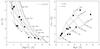 |
Fig. 1 Location of the observed stars (black dots) in the [MgFe]’, Hβ (left panel) and the Mg b, ⟨Fe⟩ (right panel) parameter space. The line grids give the predictions from simple stellar population models by Thomas et al. (2003). |
3. Analysis: kinematics, photometry, and stellar populations
In this section, we measure the stellar and ionized gas kinematics of NGC 4191 and its structural components. The stellar library we used is presented in Sect. 3.1. We first analyzed the spectra with a non-parametric fit to recover the shape of the LOSVD in each spatial bin (Sect. 3.2). Motivated by the bimodality of the recovered LOSVDs, we applied a spectral decomposition technique to investigate and characterize the presence of two kinematically distinct stellar components (Sect. 3.3). In Sect. 3.3, we also study the structural components of NGC 4191 and investigate the connection between the photometric and kinematics components. We then measured the properties of stellar populations of the two kinematic components: line strength indices, age, metallicity, and abundance ratios of α elements (Sect. 3.4). The distribution of the ionized gas is discussed in Sect. 3.5.
3.1. Stellar library
The stellar library used in the spectroscopic fit consists of 12 stars observed with Virus-W using the same observational setup of the galaxy observations. This ensures that the stellar templates had the same line spread function as the galaxy, minimizing systematic effects due to mismatch between the resolution of the stars and the galaxy spectra. This is particularly important for systems with a low velocity dispersion, where the asymmetries in the LOSVDs are comparable with asymmetries in the line spread function.
The selected stars covered a wide range of the Hβ, Mg b, [MgFe]’, and ⟨Fe⟩ parameters space, as shown in Fig. 1.
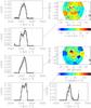 |
Fig. 2 Best-fit kinematics for the single stellar component model. The two-dimensional maps show the velocity and velocity dispersion fields. The plots on the side show some example of reconstructed non-parametric LOSVDs in the location of the field of view indicated by the dotted lines. The LOSVDs of central regions clearly show a bimodal distribution; the LOSVDs in the outer regions show high asymmetry, which can be due to the presence of an unresolved secondary kinematic component. |
3.2. Shape of the line-of-sight velocity distributions
We fitted the spectra with a non-parametric approach to recover the shape of the LOSVDs and investigate the presence of multiple kinematic components. The fitting procedure is described in Fabricius et al. (2014), and it extends the maximum penalized likelihood method by Gebhardt et al. (2000) to treat nebular emissions. After fitting and removing the continuum with a third-degree polynomial, we fitted the wavelength range from 4905−5325 Å. We modeled the LOSVD with 31 independent velocity channels and linearly combined the set of 12 stellar spectra from a library (Sect. 3.1). We successively removed stellar spectra that received low weights. The final fit was carried out with six templates. As a result of the high S/N of the data after binning (typically 90 per Å), we did not employ any penalization. For a number of bins the derived LOSVDs show a clear bimodal structure expressed as a double peak.
These bifurcated LOSVDs are more evident in the inner regions of the galaxies (r< 10′′) and are spatially consistent with the regions where the sigma peaks were detected. For the regions outside 10′′, the LOSVDs are strongly asymmetric, consistent with the interpretation that the galaxy contains two counter-rotating stellar components.
Figure 2 shows the shape of the LOSVDs in some spatial bins. To measure the mean kinematics along the line of sight, we refitted the spectra by parametrizing the LOSVD in each bin with a Gaussian function plus high-order Gauss-Hermite moments. The fit was made using a modified version of the penalized pixel-fitting code of Cappellari & Emsellem (2004) that included simultaneous fits to the ionized gas emission lines. Figure 2 shows the velocity and velocity dispersion fields obtained with the parametric fit. The two peaks in the velocity dispersion profile discovered by Krajnović et al. (2011) are visible, slightly offset by ≈ 1′′ towards the southeast with respect to the galaxy photometric major axis. The velocity field is complex and is not consistent with a single rotating component, even if high-order moments are taken into account in the LOSVD parametrization. This again supports the assumption that the components are kinematically decoupled.
3.3. Kinematics and photometry of the counter-rotating stellar components
Driven by the results of Sect. 3.2, we applied a spectral decomposition technique to investigate and characterize the presence of two kinematically distinct stellar components.
The spectral decomposition described in Sect. 3.3.1 returns for each spatial bin the kinematics, spectra, and normalized flux contribution of the two stellar components. We also fit the intensities of the emission lines and their mean velocity and velocity dispersion. We used the same spectral library for the two components and let the code select the most appropriate stellar template for each of them.
In Sect. 3.3.2 we associate these two kinematic components with the galaxy structural components derived from a photometric decomposition.
3.3.1. Spectral decomposition technique
The parametric fit of the stellar kinematics and the separation of two kinematic stellar components is made using the spectral decomposition technique developed in Coccato et al. (2011), implemented as modification to the penalized pixel-fitting code (Cappellari & Emsellem 2004).
The technique builds two optimal templates by linear combination of stellar spectra from an input library (see Sect. 3.1). The two templates are convolved with two independent LOSVDs, which are parametrized by two independent Gaussian functions. The convolved templates are then multiplied by Legendre polynomials to account for the shape of the continuum. Our implementation includes Gaussian functions that are added to fit the ionized gas emission lines Hβ and [O III]λλ4959,5007 Å. The best-fit model is recovered using the Levenberg-Mardquart χ2 minimization. The procedure allows the flux of the two components either to be free parameters in the fit or to be constrained to specified values or within a certain range. The code returns the best-fit values for the stellar kinematics and the best-fit spectra of the two stellar components, which are used in Sect. 3.4 to derive their stellar populations. The code also returns the light contribution of one component relative to the total galaxy spectrum. If we label the two components A and B, the code returns  , where IA and IB are the flux of the two components. By construction, FB = 1 − FA.
Our technique has been successfully applied to distinguish counter-rotating stellar disks in galaxies (Coccato et al. 2011, 2013; Pizzella et al. 2014), stars from the bulge and disk (Fabricius et al. 2014), and stars from the host galaxy and the surrounding polar disk (Coccato et al. 2014).
To obtain a reasonable and stable fit for the special case of NGC 4191, it is necessary to constrain the flux ratio of the two kinematic components by performing an independent photometric decomposition (Sect. 3.3.2). This is due to a degeneracy between the parameters that describe the kinematics and the stellar populations of the two components. The same approach has been adopted in Katkov & Chilingarian (2012) and Coccato et al. (2014).
Best-fit parameters of the photrometric decomposition of NGC 4191.
3.3.2. Photometric contraints
The aim of this section is to perform a photometric decomposition of NGC 4191 to constrain the flux parameter FA in the spectral decomposition code.
We acquired a g-band image (the closest match to the VIRUS-W wavelength range) from the SDSS DR7 archive and analyzed it using the 2D image-fitting code Imfit (Erwin 2015). The fitting procedure includes the convolution for a Moffat point spread function (PSF) computed using the median FWHM and β values measured from stars in the same image.
The best-fit model is obtained by adopting three components: a bulge with a Sérsic profile, one inner exponential disk, and one outer exponential disk. In the fitting procedure, the center was kept fixed for all the three components. The position angle and the ellipticity of the three components are independent, but constant with radius.
The structural parameters of the best-fitting components are given in Table 1, and the best-fit model is shown in Figs. 3 and 4. The residual map of Fig. 3 highlights a spiral-arm pattern, indicating the presence of faint spiral arms and dust in this galaxy, despite its classification as S0.
Our photometric decomposition represents an improvement of the previous single-component model by Krajnović et al. (2013). One way to evaluate the relative goodness-of-fit of different models to the same data is by information-theoretic measures such as the Akaike information criterion (AIC) or the Bayesian information criterion (BIC), both of which are output by Imfit at the end of the fitting process. Unlike the χ2 statistic, AIC and BIC do not require that the models that are compared are nested. The absolute values of these statistics are irrelevant; what matters is the relative value, with lower values indicating a better match to the data. Traditionally, ΔAIC = AIC1 − AIC2< − 10 is taken as an indication for the clear superiority of model 1 over model 2. We find that the Sérsic + two exponential model is clearly favored. For the g-band image, the three-component model has ΔAIC = −1442 compared to the Sérsic + single-exponential model and ΔAIC = −15 006 compared to the single Sérsic model. The values for the BIC are similarly high: ΔBIC = −1398 and −14 919, respectively.
Figure 5 provides additional support to the choice of the three-component model over one- or two- component models. It shows the radial profiles of ellipticity and position angle as measured from the g-band image and from the various models. The single Sérsic model in particular only poorly reproduces the position angle radial variation, and the two-component model does not reproduce the change of ellipticity as nicely as the three-component model for 25′′<a< 30′′ and a> 45′′. To constrain the flux parameter F in the spectral decomposition, we therefore used the three-component model.
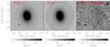 |
Fig. 3 Result of the photometric decomposition of NGC 4191. Left panel: SDSS g image; central panel: best-fit model; right panel: normalized residuals (data – model)/model. North is up and east is left. |
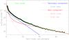 |
Fig. 4 Results of the photometric decomposition. Filled circles: surface brightness radial profile measured on the SDSS g-band image with the iraf task ellipse. The blue curve is the best-fitting inner disk component, the red dashed curve is the best-fitting Sérsic bulge, and the red dot-dashed curve is the outer disk component. The green curve is the sum of all the best-fitting components. Red and blue curves represent the profiles of the adopted definition for the main and secondary kinematics components, respectively. |
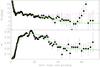 |
Fig. 5 Comparison between the radial profile of ellipticity (top panel) and position angle (bottom panel) obtained with different photometric models. Filled circles: surface brightness radial profile measured on the SDSS g-band image with the iraf task ellipse. Green line: three-component model, orange dashed line: two-component model, magenta dashed line: single-component model. |
We define as the main kinematic component the sum of the bulge and outer disk and as the secondary kinematic component the inner disk. The main kinematic components contains the ~ 64% of the total galaxy luminosity, whereas the secondary kinematic component contains the ~ 36% of the total galaxy luminosity. The particular association of the inner disk component with the counter-rotating kinematic component is driven by its relative local luminosity. From the observed peaks in the LOSVDs we know that the two components have flux ratios between 1:3 and 1:1. Other combinations, such as defining the secondary component as the sum of the two disks, would have set one of the components below a detection limit (F< 0.15, see Appendix A), which is inconsistent with the observations.
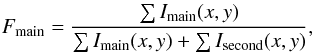
At each position (x,y) in the field of view, we can define the fraction of galaxy surface brightness contributed by the main and secondary components as 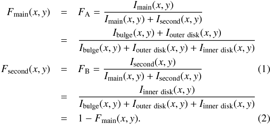 In Fig. 6 we show the radial trend along the major axis of Fsecond.
The results of the photometric decomposition can now be used to constrain the spectral decomposition analysis. For a given spatial bin, we constrain the parameter FA in the spectral decomposition code to be within the range Fmain − 0.05 <FA<Fmain + 0.05; Fmain is given by
 where the sum is done over all the spaxels contributing to a given spatial bin.
 |
Fig. 6 Radial profiles of the relative flux contribution of the secondary stellar components Fsecondary. The contribution of the main component is Fmain = 1 − Fsecondary by construction. |
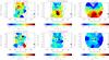 |
Fig. 7 Result of the spectral decomposition of NGC 4191. Velocity (top panels) and velocity dispersion (bottom panels) maps for the main stellar component (left panels), secondary counter-rotating stellar component (central panels), and counter-rotating ionized-gas component (right panels) are shown. Spatial bins with S/N lower than 25 per Å are not shown for the stellar components. The horizontal bars in the color scale at the bottom of each panel indicate the mean error. |
3.3.3. Kinematics of the counter-rotating stellar components
Figure 7 shows the kinematics of the two stellar components as obtained from the spectral decomposition fit.
The main galaxy component, which consists of the combination of the Sérsic bulge and the large-scale exponential disk, is more luminous. It is characterized by a rotation amplitude of ~ 70kms-1, with some scatter, and an average velocity dispersion of ~ 120kms-1.
The secondary galaxy component, which is represented by the inner exponential disk, is less luminous, and it counter-rotates with respect to the main stellar component. It has a rotation amplitude of ~ 130kms-1 and an average velocity dispersion of ~ 90kms-1. The direction of rotation is aligned with that of the ionized gas.
As an additional test, we performed the spectral decomposition using the constraints from the two-component photometric model. Although the main kinematic results are consistent with those presented above, the two-dimensional kinematics maps obtained with the two-component photometric model have higher noise. This is due to the poorer quality of the photometric fit, which translates into a larger uncertainty in constraining the light content of the counter-rotating stellar components.
3.4. Stellar populations of the counter-rotating stellar components
We measured the Hβ, Mg b, Fe5270, and Fe5335 line-strength indices on the optimal template of each stellar component returned by the spectral decomposition code. The spectra were broadened with a Gaussian function to match the spectral resolution of the Lick system (8.4 Å, Worthey & Ottaviani 1997). From this we obtained two sets of indices in each spatial bin, one set for each kinematic component.
Measurements were scaled to the Lick system by comparing the line strength indices measured in the spectra Lick standard stars HD 102870 and HD 125560 obtained with VIRUS-W with those published by Worthey et al. (1994). The offsets are −0.35 ± 0.13 Å (Hβ), −0.05 ± 0.01 Å (Mg b), −0.02 ± 0.15 Å (Fe5270), and −0.06 ± 0.12 Å (Fe5270). We applied this correction to the Hβ and Mg b indices, but not for the metal indices, because they are negligible considering the measurement errors.
In Fig. 8 we show the combined indices Hβ, Mg b [MgFe]’, and ⟨Fe⟩ of the two stellar components. The scatter in the plots is large, reflecting the uncertainties in our measurements. In particular, we note that the scatter in the measurements in the Mg b⟨Fe⟩ plane of Fig. 8 is larger for the secondary component. This is probably due to a combined effect of i) radial gradients that are more pronounced for the secondary component (see below); and ii) the secondary component being on average the less luminous, and therefore the errors in the measurements are larger.
Figure 8 also compares our measurements to the predictions of stellar population models (Thomas et al. 2003). This allows us to derive their two-dimensional maps of age, metallicity, and abundance ratios of α elements, which are shown in Fig. 9. Figures 8 and 9 do not show the results on those spatial bins where the S/N is lower than 25 per Å. In Fig. 9 we also compute median values within elliptical annuli to highlight the radial gradients in the properties of the stellar populations. The error in each elliptical bin is computed as the maximum between i) the scatter of the measurements within that elliptical bin; and ii) the weighted mean error  , where σi are the individual measurements errors in age, [Z/H], and [α/Fe].
The properties of the stellar populations of the two counter-rotating stellar components are very similar, as shown by Figs. 8 and 9. Because the scatter in the two-dimensional maps is large and a direct comparison is difficult, we compare average quantities. Metallicities and abundances of α elements are consistent with solar, without significant radial gradients. Their mean values are ⟨[Z/H]⟩ main = 0.02 ± 0.09 dex, ⟨[Z/H]⟩ second = −0.1 ± 0.2 dex, ⟨[α/Fe]⟩ main = −0.05 ± 0.05 dex, and ⟨[α/Fe]⟩ second = −0.02 ± 0.05 dex. On the other hand, the age radial profiles show a mild indication of radial gradients. The age of the stars in the main component ranges from ~ 12 Gyr in the central regions down to ~ 6 Gyr at 21′′. Outside 21′′, the age rises again, but the uncertainties at these radii become too large to derive conclusive results. One possible explanation is that if the observed increase in age is real, it might be due to accretion of old stars, which were accreted in the same rotation direction as the main component. The age of the stars in the secondary component ranges from ~ 12 Gyr in the central regions down to ~ 3 Gyr at 21′′, remaining nearly constant afterward. We compared the mean ages of the two components within 21′′, which can be considered the upper limit for trusting age measurements in the main component. We found ⟨age⟩ main(R< 21′′) = 10 ± 3 Gyr and ⟨age⟩ second(R< 21′′) = 5 ± 4 Gyr. The mean ages of the two stellar components agree within the errorbars; on the other hand, the radial profiles in Fig. 9 seem to indicate that the secondary component is systematically younger than the main galaxy by ≈ 2 Gyr at all radial bins. Implications of this age difference, if real, are discussed in Sect. 4.
By comparing the mean properties of the stellar populations with the model predictions by Maraston (2005) assuming a Salpeter initial mass function, we can derive the mean values of the stellar mass-to-light ratios of the two components in the g band: ⟨ M/L∗ ⟩ main = 6.7 ± 2.5, ⟨ M/L∗ ⟩ second = 3.3 ± 2.5. These informations, combined with the luminosity of the two components measured in Sect. 3.3.2 and the adopted distance of 42.4 Mpc, allow us to estimate their masses: Mmain = 6.2 ± 2.3 × 10¹⁰M⊙ and Msecond = 1.0 ± 9.4 × 10¹⁰M⊙; the main stellar component is aboutsix times more massive than the secondary component.
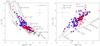 |
Fig. 8 Line strength indices of the two counter-rotating stellar components in NGC 4191. Blue filled circles and red open diamonds refer to the main and secondary component, respectively. The error bars represent the mean errors in the measurements. The line grids represent the predictions of simple stellar population models (Thomas et al. 2003). Spatial bins with S/N lower than 25 per Å are not considered. |
3.5. Kinematics and distribution of the ionized gas
The spectral decomposition routine also fits the ionized gas emission lines. The gas component (see Fig. 7) rotates in the same direction as the secondary stellar component with an amplitude of ~ 150kms-1. The velocity dispersion decreases with radius: from ~ 60kms-1 in the center down to ~ 30kms-1 in the outskirts. The high value of the velocity dispersion measured in the inner 1′′ (~ 100kms-1) is probably due to the seeing and the limited spatial resolution.
The emission lines are very weak, therefore it was necessary to spatially bin the data to measure their kinematics as in the case of the stars. For convenience, we adopted the same spatial binning as for the stellar component to measure the gas kinematics. However, this coarse binning prevents us from investigating the spatial distribution of the emission lines. We therefore reanalyzed the gas distribution on a finer spatial grid and measured the equivalent widths of the Hβ [O III]λ4959, and [O III]λ5007 Å emission lines on this latter spatial binning.
Figure 10 shows the spatial distribution of the [O III]λ5007 Å emission line equivalent widths, which is the most intense. Although the outer regions are dominated by the noise due to the lower S/N of the data, an elongated ring-like structure (or possibly a spiral arm structure) with three blobs is visible within 25′′. The position angle of the structure, using the two brightest blobs in the equivalent width map as reference, is 8.0°, which is very close to the position angle of the secondary component, that is, 7.8° (Table 1). This strengthens the association of the ionized-gas component to the secondary stellar component.
Interestingly, a similar spiral-like structure with the same size and orientation is observed in the residual map of Fig. 3; this is consistent with the concentration of gas along spiral arms. Unfortunately, the spatial binning we adopted for the stellar population studies does not have enough spatial resolution to resolve the spiral arms and separate their stellar population from that of the rest of the galaxy.
It is interesting to compare, although qualitatively, the distribution of emission lines of NGC 4191 with those of other stellar counter-rotating galaxies studied so far. The distribution of the ionized gas in NGC 4191 resembles those of NGC 3593 and NGC 5719, where the gas is also distributed along a ring-like structure with presence of blobs. In addition, for NGC 5719 the location of the most intense blobs coincides with that of the youngest stars. For NGC 4550, the gas is irregular distributed, with no signature of ring-like or spiral-like structures. NGC 4550 also is the galaxy with the two oldest stellar components.
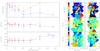 |
Fig. 9 Properties of the stellar populations of the counter-rotating components in NGC 4191. Left panels: median values of age (top panel), [Z/H] (middle panel) and [α/Fe] (bottom panel) within elliptical annuli for the main (red line) and secondary (blue line) stellar components. Right panels: two-dimensional maps of the stellar population properties. The dashed lines indicate the elliptical annuli used in computing the median values presented in the left panels. Spatial bins with S/N lower than 25 per Å are not considered in the analysis. |
4. Discussion and conclusions
The LOSVDs of NGC 4191 are complex and suggest the presence of two kinematically decoupled stellar components. Their properties have been investigated with the aid of a non-parametric fit (Fabricius et al. 2014) and a spectral decomposition technique (Coccato et al. 2011).
We also performed a parametric photometric decomposition of the surface-brightness distribution of NGC 4191. Our detailed analysis revealed three structural components that were overlooked in previous studies: a Sérsic bulge and two exponential disks of different scale lengths. Faint spiral structures (stars and dust) are also visible from the residual map.
We then linked the photometric components to the kinematic components unveiled by the spectroscopic analysis. The intensity of the double peaks in the LOSVDs allowed us to associate the bulge and the outer exponential disk with the main kinematic component. Together they represent the ~ 64% of the total galaxy luminosity. We then associated the inner exponential disk with the secondary kinematic component, which represents the ~ 36% of the total galaxy light.
The information on the photometry allowed us to constrain the relative light contribution of the two kinematic components in the spectral decomposition fit. This decreases the degeneracy between the various fitting parameters that characterize the two components (kinematics, surface brightness, and stellar populations) and allowed us to obtain a more reliable fit.
We found evidence that the two kinematic components in NGC 4191 counter-rotate with respect to each other. The secondary component rotates faster and in the same direction as the ionized gas. The main component rotates more slowly and has a higher velocity dispersion, which is consistent with hosting also bulge stars.
The properties of the stellar populations of the two kinematic components are very similar, although the large uncertainties in the measurements prevent us from making strong claims. We azimuthally averaged the measurements onto elliptical bins to reduce the statistical noise and highlight the presence of radial gradients. Figure 9 gives a tentative indication that the luminosity-weighted ages of the stars in the secondary disk are systematically lower than those of the main components at all radii. We can explain the age difference between the two components with the following scenario.
The combination of kinematics and stellar populations gives us clues on the formation mechanism of NGC 4191. Our data favor the scenario in which a disk galaxy (represented by the main kinematic component, i.e., the bulge plus the outer disk) acquired material (either gas/star accretion or galaxy mergers) from the outside onto a retrograde orbit, which formed the counter-rotating secondary component. At first glance, this scenario is the same as those of the other counter-rotating systems studied so far (Coccato et al. 2011, 2013; Katkov et al. 2013; Pizzella et al. 2014). However, there are some important differences between NGC 4191 and these other galaxies.
First, the age radial gradients observed in NGC 4191 are much steeper than those observed in other systems. Moreover, the age gradient of the secondary component is negative, whereas in the other systems it is positive. This is indicative of an inside-out star formation process for the secondary disk and favors the gas accretion scenario over major merger. A nearly 1:1 merger in fact would have redistributed the stars along all directions, smoothing any significant age gradient.
Second, there are almost no differences in the metallicity and α-elements overabundance ratio between main and secondary components, whereas differences were observed in other galaxies. In other galaxies, the scenario that better explained the differences in [Z/H] and [α/Fe] between the main and secondary components is gas accretion from a cosmic gas reservoir or from a nearby gas-rich companion. The case of NGC 5719 offers the best example of such a scenario: we observed the ongoing gas stripping process from its nearby companion that forms the counter-rotating stellar disk (Vergani et al. 2007; Coccato et al. 2011). In contrast, the data for NGC 4191 suggest that the accreted gas has an origin in common with the gas that formed the main galaxy component.
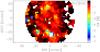 |
Fig. 10 Distribution of the [O III]λ5007 Å emission line. The gas is distributed on a ring-like structure aligned with the photometric major axis of the secondary component (see text for details). |
The observed properties of NGC 4191 can be interpreted in light of cosmological simulations (Algorry et al. 2014). The main galaxy component is formed by accretion of gas from two filaments that have a very similar chemical composition. As time passes, each filament torques the other in opposite directions, resulting into a double accretion with opposite spin. Initially, the accretion from the two filaments occurs at the same time. The collisional nature of the gas ensures that only one stellar component forms from gas whose properties is a mixture of that of the two filaments, and with the spin dictated by the most massive filament. After a while (~ 2 Gyr, considering the measured age difference between the two components in each radial bin), the accretion along one of the filaments stops.
The accretion process continues along the counter-rotating filament, which wipes out the remaining gas and forms the secondary counter-rotating component. The star formation occurs inside-out, as suggested from the negative age gradient; the newly born stars have properties very similar to those of the main component, because the gas is a mixture of that of the second filament and what remained from the first filament. Moreover, the formation of the secondary component must have occurred immediately after the formation of the main component and very rapidly, without leaving the stars of the first component enough time to reprocess and enrich the gas with metals and/or α elements. This is consistent with the relative small age difference between the two components and their equal and constant [Z/H] and [α/Fe] radial profiles. The rapid star formation process and the solar abundances and metallicity measured for the stellar populations imply that the infalling gas was already enriched, because otherwise there would not be enough time to reach the measured values of [Z/H] and [α/Fe].
The hypothesis where the main component formed first is consistent with the observed properties of the photometric components: the position angles are slightly different and the ellipticities of the Sérsic bulge and outer disk are smaller than that of the secondary component (inner disk, see Table 1). The most likely interpretation is that the bulge is triaxial and the disks have different thickness (the external disk being the thickest). This agrees with the proposed formation scenario in which the main component formed first and had more time to heat up its disk during the accretion of the gas that originated the secondary component. Gas accretion can indeed heat the host stellar disk during the formation of a counter-rotating component (e.g., Thakar & Ryden 1996).
To conclude, we would like to remark on the importance of distinguishing and measuring the properties of individual components in multispin galaxies to understand their formation mechanisms. The special case of NGC 4191 also supports the validity of the double-peaked signature in the velocity dispersion field associated with zero-velocity rotation as a selection criterion for identifying counter-rotating galaxies. This is very useful for large integral field spectroscopic surveys to provide a statistically completed census of counter-rotating galaxies in the nearby Universe.
The spectral resolution of VIRUS-W below 4800 Å deteriorates up to σinstr ~ 70kms-1. We tested that restricting the wavelength range to 4800−6040 AA has negligible effects on our results.
We define the noise (rms) as the standard deviation of the residuals between the galaxy observed spectrum (normalized to its median value) and the best-fit model. The actual computation on the wavelength region used in the fit and with the robust_sigma IDL routine. This value of rms is converted into a proxy for the S/N per angstrom by  , where 0.178 is the inverse dispersion in Å pixel-1.
References
- Algorry, D. G., Navarro, J. F., Abadi, M. G., et al. 2014, MNRAS, 437, 3596 [NASA ADS] [CrossRef] [Google Scholar]
- Bertola, F., Buson, L. M., & Zeilinger, W. W. 1992, ApJ, 401, L79 [NASA ADS] [CrossRef] [Google Scholar]
- Bryant, J. J., Owers, M. S., Robotham, A. S. G., et al. 2015, MNRAS, 447, 2857 [NASA ADS] [CrossRef] [Google Scholar]
- Bundy, K., Bershady, M. A., Law, D. R., et al. 2015, ApJ, 798, 7 [NASA ADS] [CrossRef] [Google Scholar]
- Cappellari, M., & Copin, Y. 2003, MNRAS, 342, 345 [NASA ADS] [CrossRef] [Google Scholar]
- Cappellari, M., & Emsellem, E. 2004, PASP, 116, 138 [NASA ADS] [CrossRef] [Google Scholar]
- Cappellari, M., Emsellem, E., Krajnović, D., et al. 2011, MNRAS, 413, 813 [NASA ADS] [CrossRef] [Google Scholar]
- Coccato, L., Morelli, L., Corsini, E. M., et al. 2011, MNRAS, 412, L113 [NASA ADS] [CrossRef] [Google Scholar]
- Coccato, L., Morelli, L., Pizzella, A., et al. 2013, A&A, 549, A3 [NASA ADS] [CrossRef] [EDP Sciences] [Google Scholar]
- Coccato, L., Iodice, E., & Arnaboldi, M. 2014, A&A, 569, A83 [NASA ADS] [CrossRef] [EDP Sciences] [Google Scholar]
- Corsini, E. M. 2014, in Multi-Spin Galaxies, eds. E. Iodice, & E. M. Corsini, ASP Conf. Ser., 486, 51 [Google Scholar]
- Crocker, A. F., Jeong, H., Komugi, S., et al. 2009, MNRAS, 393, 1255 [NASA ADS] [CrossRef] [Google Scholar]
- de Zeeuw, P. T., Bureau, M., Emsellem, E., et al. 2002, MNRAS, 329, 513 [NASA ADS] [CrossRef] [Google Scholar]
- Erwin, P. 2015, ApJ, 799, 226 [NASA ADS] [CrossRef] [Google Scholar]
- Evans, N. W., & Collett, J. L. 1994, ApJ, 420, L67 [NASA ADS] [CrossRef] [Google Scholar]
- Fabricius, M. H., Grupp, F., Bender, R., et al. 2012, SPIE Conf. Ser., 8446 [Google Scholar]
- Fabricius, M. H., Coccato, L., Bender, R., et al. 2014, MNRAS, 441, 2212 [NASA ADS] [CrossRef] [Google Scholar]
- Fisher, D., Illingworth, G., & Franx, M. 1994, AJ, 107, 160 [NASA ADS] [CrossRef] [Google Scholar]
- Galletta, G. 1987, ApJ, 318, 531 [NASA ADS] [CrossRef] [Google Scholar]
- Gebhardt, K., Richstone, D., Kormendy, J., et al. 2000, AJ, 119, 1157 [NASA ADS] [CrossRef] [Google Scholar]
- Husemann, B., Kamann, S., Sandin, C., et al. 2012, A&A, 545, A137 [NASA ADS] [CrossRef] [EDP Sciences] [Google Scholar]
- Johnston, E. J., Merrifield, M. R., Aragón-Salamanca, A., & Cappellari, M. 2013, MNRAS, 428, 1296 [NASA ADS] [CrossRef] [Google Scholar]
- Katkov, I. Y., & Chilingarian, I. V. 2012, Proc. IAU Symp., 284, 69 [NASA ADS] [Google Scholar]
- Katkov, I. Y., Sil’chenko, O. K., & Afanasiev, V. L. 2013, ApJ, 769, 105 [NASA ADS] [CrossRef] [Google Scholar]
- Krajnović, D., Emsellem, E., Cappellari, M., et al. 2011, MNRAS, 414, 2923 [NASA ADS] [CrossRef] [Google Scholar]
- Krajnović, D., Alatalo, K., Blitz, L., et al. 2013, MNRAS, 432, 1768 [NASA ADS] [CrossRef] [Google Scholar]
- Maraston, C. 2005, MNRAS, 362, 799 [NASA ADS] [CrossRef] [Google Scholar]
- Pizzella, A., Corsini, E. M., Vega Beltrán, J. C., & Bertola, F. 2004, A&A, 424, 447 [NASA ADS] [CrossRef] [EDP Sciences] [Google Scholar]
- Pizzella, A., Morelli, L., Corsini, E. M., et al. 2014, A&A, 570, A79 [NASA ADS] [CrossRef] [EDP Sciences] [Google Scholar]
- Puerari, I., & Pfenniger, D. 2001, Ap&SS, 276, 909 [Google Scholar]
- Rix, H.-W., Franx, M., Fisher, D., & Illingworth, G. 1992, ApJ, 400, L5 [NASA ADS] [CrossRef] [Google Scholar]
- Rubin, V. C., Graham, J. A., & Kenney, J. D. P. 1992, ApJ, 394, L9 [NASA ADS] [CrossRef] [Google Scholar]
- Sánchez, S. F., Kennicutt, R. C., Gil de Paz, A., et al. 2012, A&A, 538, A8 [NASA ADS] [CrossRef] [EDP Sciences] [Google Scholar]
- Thakar, A. R., & Ryden, B. S. 1996, ApJ, 461, 55 [NASA ADS] [CrossRef] [Google Scholar]
- Theureau, G., Hanski, M. O., Coudreau, N., Hallet, N., & Martin, J.-M. 2007, A&A, 465, 71 [NASA ADS] [CrossRef] [EDP Sciences] [Google Scholar]
- Thomas, D., Maraston, C., & Bender, R. 2003, MNRAS, 339, 897 [NASA ADS] [CrossRef] [Google Scholar]
- Vergani, D., Pizzella, A., Corsini, E. M., et al. 2007, A&A, 463, 883 [NASA ADS] [CrossRef] [EDP Sciences] [Google Scholar]
- Worthey, G., & Ottaviani, D. L. 1997, ApJS, 111, 377 [NASA ADS] [CrossRef] [Google Scholar]
- Worthey, G., Faber, S. M., Gonzalez, J. J., & Burstein, D. 1994, ApJS, 94, 687 [NASA ADS] [CrossRef] [Google Scholar]
Appendix A: Errors of the spectroscopic decomposition
The ability of the spectral decomposition code to measure the kinematic and properties of the stellar populations depends on many parameters. First, on the differences of the two stellar components: the more separated they are in kinematics and stellar populations, the easier it is to decouple their contribution from the observed galaxy spectrum. The spectral resolution and wavelength range of the instrument and the S/N of the observations are likewise important.
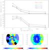 |
Fig. A.1 Top panel: median value (top panel) and standard deviation (bottom panel) of the error on the recovered velocities as a function of the velocity difference between the two simulated stellar components. Different lines represent different S/N values per Å: 480 (rms = 0.005), 120, 80, and 24 (rms = 0.1). Bottom panel: two-dimensional maps of the absolute velocity difference between the two stellar components (left panel) and the fit rms (right panel). |
We therefore simulated galaxy spectra that represent observations and the instrumental set-up as close as possible. We then performed the spectral decomposition on those simulated spectra to derive the errors on the measured quantities.
The simulated galaxy spectra were constructed by creating and adding two stellar templates broadened to have 100 kms-1 of velocity dispersion. The stellar templates were both constructed using the same star, HD 106210, observed with the VIRUS-W (to match the instrumental setup), which has line strength indices as close as possible to the mean measured values.
We then explored the parameter space defined by the velocity separation of the two components (ΔV), and the S/N. For each point (ΔV,S/N) in the parameter space we constructed a set of 100 simulated galaxy spectra by adding Gaussian noise. We then performed the spectral decomposition on these simulated spectra to derive the errors on the measured quantities. The parameter space is sampled by ΔV = 50,75,100,150,250 km s-1, and noise = 0.005,0.02,0.03,0.10, which corresponds to a S/N ranging from 480 to 25 per Å (the mean S/N of the binned spectra is 90 per Å)2.
We found that the errors on the absorption line indices do not vary much with velocity separation because the stellar populations of the two components used in the simulations are the same (i.e., there is no degeneracy with the kinematics). There is also little dependence on the S/N. The mean errors on the indices are 0.2 Å 0.4 Å, 0.2 Å, and 0.2 Å, for the Hβ, Mg b, Fe5270, and Fe5335 indices, respectively.
We found that the errors on velocity separation between the two components depend on the input velocity separation and on the S/N. Figure A.1 shows the error on the recovered velocity separation as a function of the input noise and input velocity separation. For typical values measured along the galaxy kinematic major axis, where the velocity separation is ΔV> 150kms-1 and the noise is rms < 0.05, the error on the velocity separation between the two components is ≃ 30kms-1. The error on the recovered flux of the two components is ~ 15%.
All Tables
All Figures
|
Fig. 1 Location of the observed stars (black dots) in the [MgFe]’, Hβ (left panel) and the Mg b, ⟨Fe⟩ (right panel) parameter space. The line grids give the predictions from simple stellar population models by Thomas et al. (2003). |
| In the text | |
|
Fig. 2 Best-fit kinematics for the single stellar component model. The two-dimensional maps show the velocity and velocity dispersion fields. The plots on the side show some example of reconstructed non-parametric LOSVDs in the location of the field of view indicated by the dotted lines. The LOSVDs of central regions clearly show a bimodal distribution; the LOSVDs in the outer regions show high asymmetry, which can be due to the presence of an unresolved secondary kinematic component. |
| In the text | |
|
Fig. 3 Result of the photometric decomposition of NGC 4191. Left panel: SDSS g image; central panel: best-fit model; right panel: normalized residuals (data – model)/model. North is up and east is left. |
| In the text | |
|
Fig. 4 Results of the photometric decomposition. Filled circles: surface brightness radial profile measured on the SDSS g-band image with the iraf task ellipse. The blue curve is the best-fitting inner disk component, the red dashed curve is the best-fitting Sérsic bulge, and the red dot-dashed curve is the outer disk component. The green curve is the sum of all the best-fitting components. Red and blue curves represent the profiles of the adopted definition for the main and secondary kinematics components, respectively. |
| In the text | |
|
Fig. 5 Comparison between the radial profile of ellipticity (top panel) and position angle (bottom panel) obtained with different photometric models. Filled circles: surface brightness radial profile measured on the SDSS g-band image with the iraf task ellipse. Green line: three-component model, orange dashed line: two-component model, magenta dashed line: single-component model. |
| In the text | |
|
Fig. 6 Radial profiles of the relative flux contribution of the secondary stellar components Fsecondary. The contribution of the main component is Fmain = 1 − Fsecondary by construction. |
| In the text | |
|
Fig. 7 Result of the spectral decomposition of NGC 4191. Velocity (top panels) and velocity dispersion (bottom panels) maps for the main stellar component (left panels), secondary counter-rotating stellar component (central panels), and counter-rotating ionized-gas component (right panels) are shown. Spatial bins with S/N lower than 25 per Å are not shown for the stellar components. The horizontal bars in the color scale at the bottom of each panel indicate the mean error. |
| In the text | |
|
Fig. 8 Line strength indices of the two counter-rotating stellar components in NGC 4191. Blue filled circles and red open diamonds refer to the main and secondary component, respectively. The error bars represent the mean errors in the measurements. The line grids represent the predictions of simple stellar population models (Thomas et al. 2003). Spatial bins with S/N lower than 25 per Å are not considered. |
| In the text | |
|
Fig. 9 Properties of the stellar populations of the counter-rotating components in NGC 4191. Left panels: median values of age (top panel), [Z/H] (middle panel) and [α/Fe] (bottom panel) within elliptical annuli for the main (red line) and secondary (blue line) stellar components. Right panels: two-dimensional maps of the stellar population properties. The dashed lines indicate the elliptical annuli used in computing the median values presented in the left panels. Spatial bins with S/N lower than 25 per Å are not considered in the analysis. |
| In the text | |
|
Fig. 10 Distribution of the [O III]λ5007 Å emission line. The gas is distributed on a ring-like structure aligned with the photometric major axis of the secondary component (see text for details). |
| In the text | |
|
Fig. A.1 Top panel: median value (top panel) and standard deviation (bottom panel) of the error on the recovered velocities as a function of the velocity difference between the two simulated stellar components. Different lines represent different S/N values per Å: 480 (rms = 0.005), 120, 80, and 24 (rms = 0.1). Bottom panel: two-dimensional maps of the absolute velocity difference between the two stellar components (left panel) and the fit rms (right panel). |
| In the text | |
Current usage metrics show cumulative count of Article Views (full-text article views including HTML views, PDF and ePub downloads, according to the available data) and Abstracts Views on Vision4Press platform.
Data correspond to usage on the plateform after 2015. The current usage metrics is available 48-96 hours after online publication and is updated daily on week days.
Initial download of the metrics may take a while.