| Issue |
A&A
Volume 581, September 2015
|
|
|---|---|---|
| Article Number | A11 | |
| Number of page(s) | 49 | |
| Section | Cosmology (including clusters of galaxies) | |
| DOI | https://doi.org/10.1051/0004-6361/201526080 | |
| Published online | 25 August 2015 | |
Galaxy luminosity functions in WINGS clusters ⋆,⋆⋆
1 INAF–Osservatorio Astronomico di Padova, Vicolo dell’Osservatorio 5, Padova, Italy
e-mail: This email address is being protected from spambots. You need JavaScript enabled to view it.
2 University of Padova, Department of Physics and Astronomy, Vicolo dell’Osservatorio 2, Padova, Italy
3 Centro de Estudios de Fisica del Cosmos de Aragon, Plaza de San Juan 1, 44001 Teruel, Spain
4 Kavli Institute for the Physics and Mathematics of the Universe (WPI), Todai Institutes for Advanced Study, the University of Tokyo, 113-8664 Tokyo, Japan
5 Observatoire de Genève, Université de Genève, Switzerland
6 Centro de Radioastronomia y Astrofisica, UNAM, Campus Morelia, A.P. 3-72, CP 58089, Mexico
7 Australian Astronomical Observatory, PO Box 915, North Ryde, NSW 1670, Australia
8 Niels Bohr Institute, Juliane Maries Vej 30, 2100 Copenhagen, Denmark
Received: 12 March 2015
Accepted: 26 May 2015
Abstract
Aims. Using V band photometry of the WINGS survey, we derive galaxy luminosity functions (LF) in nearby clusters. This sample is complete down to MV = −15.15, and it is homogeneous, thus facilitating the study of an unbiased sample of clusters with different characteristics.
Methods. We constructed the photometric LF for 72 out of the original 76 WINGS clusters, excluding only those without a velocity dispersion estimate. For each cluster we obtained the LF for galaxies in a region of radius = 0.5 × r200, and fitted them with single and double Schechter’s functions. We also derive the composite LF for the entire sample, and those pertaining to different morphological classes. Finally, we derive the spectroscopic cumulative LF for 2009 galaxies that are cluster members.
Results. The double Schechter fit parameters are correlated neither with the cluster velocity dispersion nor with the X-ray luminosity. Our median values of the Schechter’s fit slope are, on average, in agreement with measurements of nearby clusters, but are less steep that those derived from large surveys, such as the SDSS. Early-type galaxies out number late-types at all magnitudes, but both early and late types contribute equally to the faint end of the LF. Finally, the spectroscopic LF is in excellent agreement with the one derived for A2199, A85 and Virgo, and with the photometric LF at the bright magnitudes (where both are available).
Conclusions. There is a large spread in the LF of different clusters, however, this spread is not caused by correlation of the LF shape with cluster characteristics such as X-ray luminosity or velocity dispersions. The faint end is flatter than previously derived (αf = −1.7), which is at odds with that predicted from numerical simulations.
Key words: galaxies: clusters: general / galaxies: luminosity function, mass function / galaxies: statistics
Based on observations collected at the European Organisation for Astronomical Research in the Southern Hemisphere, Chile. Progs. ID 67.A-0030, 68.A-0139, and 69.A-0119.
Table 1 and full Fig. 1 (Fig. A.1) are available in electronic form at http://www.aanda.org
© ESO, 2015
1. Introduction
Galaxy clusters are unique laboratories to study the environmental effects on galaxy evolution. How galaxies form and evolve can be studied using a variety of techniques, one of those being the galaxy luminosity function (LF). The LF, i.e. the number density of galaxies at a given luminosity, is one of the most fundamental statistics of galaxy populations. Its shape and variation with environment provide a crucial constraint on any model of galaxy evolution.
The LF can be used as a diagnostic tool to search for changes in the galaxy population, for example, the study of the shape of the LF with respect to the cluster-centric radius can provide important insight into the dynamical processes working in clusters. Several studies show that quiescent and star-forming galaxies have very different LFs (Madgwick et al. 2002; Christlein & Zabludoff 2003). Galaxies in clusters have often been compared to galaxies in the field, at many different wavelengths, leading to results that are sometimes contradictory. De Propris et al. (1998), Christlein & Zabludoff (2003), Cortese et al. (2003) and Bai et al. (2006) found the cluster LF to be indistinguishable from field one, while other authors suggest that it has both brighter characteristic magnitudes and different faint end slopes (Valotto et al. 1997; Goto et al. 2002; Yagi et al. 2002; De Propris et al. 2003). Some studies seem to indicate, in fact, that the faint end slope of the LF is different in clusters and field, with the cluster environment being richer in faint galaxies than the field (Popesso et al. 2006; Blanton et al. 2005). However, more recently Agulli et al. (2014), studying the spectroscopic LF of Abell 85, find that the faint-end slope of the LF is consistent with that of the field.
Finally, some studies claim that the cluster LF shows little variation across a wide range of cluster properties (Colless 1989; Rauzy et al. 1998; De Propris et al. 2003; Popesso et al. 2006), while others find it depends on cluster richness, Bautz-Morgan type (Bautz & Morgan 1970), or distance from the cluster centre (Dressler 1978; Garilli et al. 1999; Lopez-Cruz et al. 1997; Hansen et al. 2005; Barkhouse et al. 2007).
Differences in the estimated parameters might be related to the contamination from background galaxies, especially in the faint part of the LF, while the bright part can suffer from superposition of other clusters along the line of sight. While this second effect is more easily taken into account, since two sequences tend to appear in the cluster colour–magnitude diagram, the first effect can only be alleviated with statistical approaches, which have large uncertainties.
In this respect, the availability of large galaxy surveys in the recent years has prompted the study of the global characteristics of galaxy clusters. In particular, we have at our disposal the large sample of the WIde-field Nearby Galaxy-clusters survey (WINGS; Fasano et al. 2006) of low redshift clusters that is particularly suited to this purpose, since galaxies have been observed over a large field around the cluster centre with the required accuracy. In the WINGS survey, we have a FWHM average seeing of ~1.2 arcsec, which converts into a spatial resolution of 1.2–1.4 kpc for our range of redshift. A reliable object classification, as well as an excellent morphological completeness and a good spectroscopic coverage make this survey the ideal place to study, in particular, cluster galaxy LFs.
The purpose of this paper is to present the LF of 72 clusters of galaxies belonging to the WINGS survey, for which we possess reliable star/galaxy classification and magnitudes up to V ~ 22. This helps us to understand whether the LF varies or not as a function of cluster characteristics such as the X-ray luminosity or the velocity dispersion. In Sect. 2 we describe the data sample we used, and in Sect. 3 we derive the LF. In Sect. 4 we present our conclusions about the universality of the fitted LF and the dwarf galaxy population. Finally, in Sect. 5, we present our LF for morphologically selected samples of galaxies and for a much more limited sample of spectroscopically confirmed cluster members.
Throughout this work we have used the cosmological parameters H0 = 70 km s-1 Mpc-1, Ωm = 0.3 and ΩΛ = 0.7.
2. Data sample
The WIde-field Nearby Galaxy-cluster Survey (WINGS) has been designed to derive the properties of galaxies in the cluster environment in the local Universe, and it is therefore of particular relevance in the context of studying the local LF. Here we briefly summarize the main survey characteristics. WINGS is a multi-wavelength project based on the analysis of deep wide-field images of nearby clusters selected from the X-ray flux-limited samples described in Ebeling et al. (1996, 1998, 2000). Their location in the sky has been chosen to minimize the contamination from the Galactic extinction (| b | ≥ 20°). Cluster redshifts are in the range 0.04–0.07. All the available data for the WINGS survey are described in Moretti et al. (2014), in particular, the spectroscopic follow-up for 48 clusters (Cava et al. 2009), as well as the photometric data in the optical (Varela et al. 2009), near infrared (Valentinuzzi et al. 2009) and U band (Omizzolo et al. 2014). Stellar masses and star formation histories have been derived for the subsample of galaxies with spectroscopy (Fritz et al. 2007, 2010, 2014).
One of the primary goals of the WINGS survey has been, since the beginning of the observations, the spectroscopical coverage of large areas in each of the sampled cluster. Cava et al. (2009) illustrates the final WINGS spectroscopic sample, which is made of 6137 galaxies (in 48 clusters) observed with two telescopes (WHT for the north sample and AAT for the south sample) with a medium resolution setup (6–9 Å). The wavelength coverage ranges from ~3800 to 6800 Å. For these galaxies, we could determine redshifts (with a median error of ~30 km s-1) and membership as described in the original paper. To maximize the probability of observing galaxies at the cluster redshift, without biasing the cluster sample, targets were selected on the basis of their properties so that background galaxies (redder than the cluster red sequence) could be reasonably avoided. In particular, the spectroscopic sample is made of galaxies with V ≤ 20 (total magnitude), Vfiber< 21.5 and (B − V)5 kpc ≤ 1.4. This last cut has been then slightly varied from cluster to cluster to optimize the observational setup. We then, a posteriori, calculated the spectroscopical completeness as the ratio of the number of spectra with a redshift determination with respect to the number of galaxies in the photometric catalogue obeying the previous criteria. This completeness is essentially independent of the distance from the cluster centre (for most clusters) and of the magnitude (see Cava et al. 2009, for a complete analysis).
2.1. Computing the luminosity function
We used the Sextractor photometric catalogue of WINGS galaxies described in Varela et al. (2009), which refers to optical (B,V) photometry of 76 cluster of galaxies, either observed with the INT telescope at La Palma, or with the 2.2 m ESO telescope at La Silla. For each detection we possess a star/galaxy classification based on the Sextractor stellarity index (Bertin & Arnouts 1996), which leads to a sample of 394 280 galaxies, 180 952 unknown objects, and 183 792 stars.
As described in Varela et al. (2009), this classification has been severely tested against other parameters and visually inspected, when possible. A careful analysis of the results demonstrates that the classification of galaxies is reliable up to V ~ 22, while for fainter objects (up to V ~ 24) no conclusion about the star/galaxy classification can safely be drawn. In particular, simulations show that a certain fraction of unclassified objects (variable with magnitude) had to be considered as made of galaxies (see Fig. 8 of Varela et al. 2009). We took this effect into account, by adding to the number of detections classified as galaxies a fraction of unknown/galaxy objects, calculated interpolating the Varela et al. (2009) points in Fig. 8, above V = 21.5. From now on in the paper the population referred to as galaxies is already corrected for this factor.
The characteristics of the galaxy population have been shown to vary with cluster-centric distance (Christlein & Zabludoff 2003; Hansen et al. 2005; Popesso et al. 2006), and this fact likely produces a bias when analysing different dynamical regions of clusters. To overcome this problem and make meaningful comparisons between clusters with different size and richness, as previously done by Popesso et al. (2006) and Barkhouse et al. (2007), we selected only galaxies located inside 0.5 × r200, defined as the radius of a sphere with interior mean density 200 times the critical density of the Universe at that redshift. We calculated the quantity r200 in Mpc from the velocity dispersion and redshift z, taken from Cava et al. (2009) using the following equation (Finn et al. 2005; Poggianti et al. 2006):  (1)where σv is the velocity dispersion of the cluster. The velocity dispersion measurement was not available for 4 out of 76 clusters, and therefore we excluded them from our analysis.
We used the VAUTO magnitude from Sextractor and applied the k-correction using the recipe given in Poggianti (1997). The correction is calculated on the basis of the (B − V) colour of each galaxy (relative to an aperture of ~10.8 kpc), which is considered a proxy for the galaxy type. We also took in account the photometric completeness as described in Varela et al. (2009). We used a fit to their Fig. 5 to derive the global completeness function for our clusters, and corrected each LF bin for this value. In what follows, we then fitted only the magnitude range (different for each cluster) where the completeness was larger than 90%. Table 1 lists this limit for each cluster. As for the field contribution, we used the number counts of extended sources in the ELaIS-S1 area, given in Berta et al. (2006). Before applying the statistical correction, we scaled the number counts to the area covered by our observations, and in particular to the area where we estimated the LF (i.e. 0.5 × r200).
The brightest cluster galaxies (BCG) always form a distinct class of objects (Fasano et al. 2010), and therefore have been excluded from our sample of galaxies.
Errors on the calculated number density have been derived following Lugger (1986) and Barkhouse et al. (2007) as  (2)where N is the corrected number of galaxies in the given bin after the completeness and field subtraction, Nnc is the original number of galaxies, Nf is the number count of the field galaxies in the given bin, and A is the area in Mpc2.
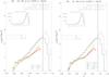 |
Fig. 1 LF for the cluster A85: the black continuous line is the original LF, the dashed line is the same LF corrected for completeness. The vertical line shows the magnitude limit (different for each cluster) at which the completeness is 90%. In red and green we show the LF of the two subsamples of galaxies and galaxies and unknown object, respectively. These two last distributions have been corrected for field contamination (whose number counts are shown in the inset). Superimposed on the red LF is the best fit that we obtained using a single Schechter function (left panel) and a double Schechter function (right panel). In the bottom right insets we give the relative parameters. |
We also derive LFs for galaxies having different morphological classes (ellipticals, S0, and later types). For a subsample of 39 124 galaxies, we were able to perform an automatic morphological classification using MORPHOT (Fasano et al. 2012), a tool that has been created for the WINGS survey. The classification is based on 21 visual diagnostics and on a parallel Neural Network machine. We refer to the original paper for details on the tool. The MORPHOT ability to classify objects obviously depends on the cluster distance, as well as on the overall photometric quality of observations. We therefore decided to use only galaxies having magnitudes brighter than the galaxy in which the MORPHOT completeness is higher than 0.5. The MORPHOT completeness is defined as the ratio between the number of galaxies classified and the number of photometric detections classified as galaxies. This limit is obviously variable within the cluster sample, but is in the interval MV = −16.5 − 17.5. In particular ~18% of the cluster sample has a limit of completeness of 50% at magnitude MV = −16.0, for the 40% the same limit is at MV = −17.0 and the remaining of the sample reach the 50% completeness at MV = −17.5. The number counts of galaxies in each morphological class have been corrected for the morphological incompleteness.
For the LF of different morphological classes, we decided to use the sample described in Calvi et al. (2011a), derived from the Millennium Galaxy Catalogue (MGC) by Liske et al. (2003), Driver et al. (2005) to perform a meaningful background subtraction. The sample is made of 3210 galaxies located in the so-called “general field” (see Calvi et al. 2011b for details about the subsample definitions) for which the morphological classification has been performed using MORPHOT.
We first calculated the morphological mix of galaxies in each magnitude bin, and then rescaled this number to the total number of galaxies expected in that bin from the number counts by Berta et al. (2006).
Finally we construct the spectroscopic LF for the subsample of 21 clusters with a spectroscopic completeness higher than 50%. To accomplish this, we used the spectroscopic information given in Cava et al. (2009) to derive the membership of our detections, and corrected for spectroscopic incompleteness as described in Cava et al. (2009) and Vulcani et al. (2011).
3. Cluster luminosity functions
3.1. Single Schechter function fit
For each cluster we calculated the LF as described in the previous section for three different classes of objects (galaxies, stars and unknown). As an example, in Fig. 1 (for all the clusters see Fig. A.1) we show the results for the cluster A85. The LF for galaxies is represented by the red line histogram, while that for galaxies plus all unknown is represented by the green line histogram.
Each LF has then be fitted up to the limiting magnitude (vertical line in Fig. 1), defined as the magnitude at which the sample is 90% complete. This number varies with the cluster distance and the quality of observations. In Fig. 1 it can be seen how the completeness correction and the field subtraction act on the final LF (dashed black line and red/green lines, respectively). The left panel of Fig. 1 shows the best fit of the galaxy LF obtained using one single Schechter (Schechter 1976) function of the form, ![Mathematical equation: \begin{eqnarray} \phi(L)=\phi^\ast \left[\left(\frac{L}{L^\ast}\right)^{\alpha} \exp \left(\frac{-L}{L^\ast}\right)\right] , \end{eqnarray}](/articles/aa/full_html/2015/09/aa26080-15/aa26080-15-eq35.png) (3)which describes the number of galaxies per unit volume (φ) as a function of the galaxy luminosity L, the characteristic galaxy luminosity L∗, corresponding to the knee of the LF, and the slope of the LF at low luminosities α. If we let the Schechter parameters free to vary, we obtain unphysical results in clusters that have a poor galaxy population, or where a hint for the presence of a secondary sequence of a background cluster is present. We excluded from the calculation of the mean/median Schechter parameters fit these clusters (49/72), i.e. those having errors in the derived
(3)which describes the number of galaxies per unit volume (φ) as a function of the galaxy luminosity L, the characteristic galaxy luminosity L∗, corresponding to the knee of the LF, and the slope of the LF at low luminosities α. If we let the Schechter parameters free to vary, we obtain unphysical results in clusters that have a poor galaxy population, or where a hint for the presence of a secondary sequence of a background cluster is present. We excluded from the calculation of the mean/median Schechter parameters fit these clusters (49/72), i.e. those having errors in the derived  and α larger than 2.0 and 0.275, respectively.
Figure 2 shows the distributions of (upper panels) and α parameters (lower panels) for two subsamples of objects, i.e. galaxies (black continuous line) and galaxies plus unknown (superimposed as green dashed histogram in the right panel). Our median (mode) values for the LF characteristic luminosity and slope are  (− 21.25) and α = −1.15(− 1.30) considering the sample of galaxies, whereas becomes brighter (−21.81, − 21.75 for median and mode) also including unknown objects. We also calculated the weighted mean of and α using as weight the error on the derived quantity, obtaining
 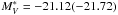 and α = −1.35( − 1.39) for the two subsamples of pure galaxy population and galaxy plus unknown. In this case, we did not exclude clusters with a poor determination of the parameters.
To compare these results with literature data we considered first the Virgo, Fornax, and the 2dFGRS surveys (Trentham & Hodgkin 2002; Ferguson 1989; Deady et al. 2002; De Propris et al. 2003) of nearby clusters. To make this comparison, we transformed their B band data to our V band using a value of (B − V) = 1 (that is the typical colour of a single stellar population with an age larger than ~6 Gyr, with solar metallicity and Salpeter IMF; see Bruzual & Charlot 2003 models) and took the different cosmology into account. We find that our estimates are in agreement with the literature where the LF has been calculated up to a very faint magnitude limit, as shown in Fig. 3. There are, however, different results in the literature, e.g. those coming from Coma (Mobasher et al. 2003) and other clusters (Garilli et al. 1999; Goto et al. 2002; Paolillo et al. 2001), where the slope turns out to be shallower than that found in Virgo, Coma, and the 2dFGRS survey. In fact, after having converted the data from Garilli et al. (1999), Goto et al. (2002), Paolillo et al. (2001) using the relation B = g + 0.54 (Liske et al. 2003), and the (B − V) colour term described above, we find a value for in broad agreement with all the data except Goto et al. (2002).
The slope is in agreement with studies based on fields of similar size (Trentham & Hodgkin 2002; Ferguson 1989; Deady et al. 2002; De Propris et al. 2003), while it turns out to be steeper than the slope found for core regions (Garilli et al. 1999; Goto et al. 2002; Paolillo et al. 2001), where evolutionary processes build up the cD galaxy leading to the disruption of dwarf galaxies. Coma (Mobasher et al. 2003) lies in the region of shallower slopes, but this could be due to selection effects, since the spectroscopic sample is based on the R-magnitude, while the LF refers to the B band (Driver & De Propris 2003).
Our magnitude limit lies between MV = −13.6 and MV = −15.15, which is the limiting magnitude for the Coma data here considered. Virgo and Fornax have even deeper magnitude limits, and are fitted with nearly the same MV. Paolillo et al. (2001) sample has a limiting magnitude of MV = −17, and Garilli et al. (1999), De Propris et al. (2003) sample reaches MV = −18. There is, therefore, the possibility that in these clusters the rising faint end of the LF is not visible, thus making their Schechter’s slope α flatter. The mean errors in the derived fit are 0.55 and 0.09 in MV and α, respectively.
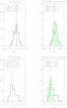 |
Fig. 2 Distribution of |
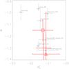 |
Fig. 3 Comparison with literature data, homogenized to the same photometric band and cosmological parameters. The squared point refers to the WINGS median values, the circle is the mode, while the triangle is the weighted mean. Errors are the mean errors in the derived parameters. |
3.2. Double Schechter function fit
The left panel of Fig. 1 clearly shows that a single Schechter fit does not reproduce the details of the LF, and, in particular, the steepening of the faint end of the LF and the central plateau.
Recent studies on nearby clusters (see Boselli et al. 2008; Penny et al. 2011; Agulli et al. 2014, among others) have indeed confirmed that the LF steepens at faint magnitudes, especially when moving towards the external regions of the cluster.
Therefore, we fit our LFs using a double Schechter function (see Driver et al. 1994; Hilker et al. 2003; González et al. 2006; Popesso et al. 2006; Barkhouse et al. 2007, among others). The function has the following form: ![Mathematical equation: \begin{eqnarray} \phi(L)=\phi^\ast \left[\left(\frac{L}{L_b^\ast}\right)^{\alpha_b} \exp \left(\frac{-L}{L_b^\ast}\right)+\left(\frac{L_b^\ast}{L_{\rm f}^\ast}\right)\times\left(\frac{L}{L_{\rm f}^\ast}\right)^{\alpha_{\rm f}} \exp\left(\frac{-L}{L_{\rm f}^\ast}\right)\right] , \end{eqnarray}](/articles/aa/full_html/2015/09/aa26080-15/aa26080-15-eq57.png) (4)where the number of galaxies per unit volume φ depends both on the characteristic magnitude and slope in the bright part of the LF (
(4)where the number of galaxies per unit volume φ depends both on the characteristic magnitude and slope in the bright part of the LF ( and αb, respectively) and on the characteristic magnitude and slope in the faint part (
 and αf, respectively). Table 1 lists the results of our fits for all clusters. In Col. 1 we identify the cluster, in Cols. 2 and 3 we list the area (in Mpc) over which the LF has been calculated and the dwarf-to-giant ratio (DGR), respectively. The last quantity has been calculated as the ratio between the number of objects with absolute V magnitude brighter than –19.0 and the number of objects fainter than this limit (see Poggianti et al. 2001) but brighter than –15.15, which is the faintest magnitude limit reached in all clusters. In Cols. 4 to 11 we give the parameters of the best fitting double Schechter fit
  , Err(), αb, Err(αb),
  , Err(), αf and Err(αf). Finally, the last four columns give the total number of galaxies analyzed Ngx, the cluster velocity dispersion σv (in km s-1), the cluster X-ray luminosity LX, and the absolute magnitude limit Mlim, up to which the LF has been fitted.
The last six rows give the median and mode results for two subsamples: the one including only objects classified as galaxies (corrected for the fraction of unknown that can be classified as galaxies), and the one where all objects (i.e. galaxies and unknown objects, excluding stars) are included. For both subsamples, we give the parameters of the free fitting and the parameters of the fit obtained imposing αb = −1.10.
We first fitted the double Schechter function to each LF letting all parameters free, and then considered good fits those with errors in the magnitudes lower than 2.5 and errors in the slopes lower than 1.0. We were able to fit 41/72 clusters and obtained median values of −21.15 and −16.30 for the bright and faint end  , while for the slopes the values are −0.97 and −0.6, respectively. These values together with the mode values are given in Table 1.
We compared our results with those by Popesso et al. (2006) and Barkhouse et al. (2007), after having transformed their magnitude values to the V band (and using our cosmology). For the values given in Popesso et al. (2006) we converted the g magnitude using the transformation V = g − 0.565(g − r), while for those taken from Barkhouse et al. (2007), we used (B − V) = 1 and (B − R) = 1.8. This last value is the mean colour calculated by López-Cruz et al. (2004) for the same clusters analyzed in Barkhouse et al. (2007) at R = 17. Both Popesso et al. (2006) and Barkhouse et al. (2007) calculated their LFs inside the same physical region in each cluster (i.e. r200 or r500, in the first case, and between 0.2 and 0.4 r200 and 0.4 and 0.6 r200 in the second case).
When compared with these data, our results seem to favour a brighter (0.35–1.0 mag) magnitude for the bright characteristic magnitude of the LF and a fainter magnitude for the faint end part (0.4–0.9 mag, see Fig. 4). At the same time, the slope in the bright regime is compatible with the values given in literature, while it is flatter in the faint end regime (see, for example, values given in Popesso et al. 2006; Barkhouse et al. 2007, but also Boué et al. 2008, for results more similar to ours).
To better compare our findings with others, we run a fit after having imposed a bright end slope of αb = −1.10, corresponding to the mode value of our LFs fits and to the value found by Popesso et al. (2006) within r200. In this way we were able to fit 56/72 clusters (selected using the same criterion described above).
Figure 4 shows the comparison between our derived parameters (median values) for the LF faint end (upper panel) and for the bright end (lower panel). In both cases we show the median values for the galaxy (including the unknown galaxies) population in red, and the population of galaxies and unknown object, without the stellar component, in green. Squares refer to values derived using a fixed αb = −1.10 and triangles to values derived leaving free all parameters. The purple triangle shows, finally, the weighted mean of the fitted parameters, which we only calculated for the subsample of galaxies and leaving free the bright end of the LF. If we consider the weighted mean, the bright part of the LF shows a much better agreement with the values derived by Barkhouse et al. (2007), but in the faint part the results again show a flatter slope.
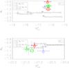 |
Fig. 4 Comparison with literature data, homogenized to the same photometric band and cosmological parameters. Squared point refer to the WINGS median values of the galaxies (including the unknown galaxies) subsample, the triangle to the subsample all objects of galaxies and unknown sources, excluding stars. When fixing the αb the |
 |
Fig. 5 Variation of αf (left panels) and MV (right panels) with σv (upper panel) and LX (lower panel), with superimposed the least-squares fit. |
The derived best-fit parameters show a good agreement in the bright part of the LF, where both samples of pure galaxy population and the one including unknown objects have  and a slope of –1.10. As for the faint part of the LF, we find fainter characteristic magnitudes and slightly flatter slopes, even after having fixed the bright end slope.
The net effect of including more galaxies taken from the unknown class in the WINGS sample is to have a brighter characteristic magnitude in the bright end part of the LF and more or less the same slope in the faint end part. This result is somewhat unexpected, since unknown galaxies included in the second sample are mainly dwarf galaxies, which should have the effect, if any, to steepen the faint end LF. However, the double Schechter fit tries to fit simultaneously the two parts, such that to better reproduce the steepening of the faint end it also moves the bright end magnitude towards the faint end. What we find, in fact, are LF flatter than those found so far, but with a more pronounced central plateau.
The main concern in the Schechter fitting is related to the large errors on the single fits, which we derived leaving free to vary all parameters of the double Schechter function (or fixing one of them, the bright end slope), as can be seen from Table 1. This statistical effect is known, and can be solved by constructing a composite LF, where all clusters contribute, thus giving much stronger constraints on the resulting LF in particular for their faint end. However, the composite LF is meaningful only in the case in which we think that the cluster LF is universal, otherwise differences would be cancelled out and the derived parameters would be a sort of average behaviour. The next section is dedicated to a more detailed discussion on the universality of the WINGS cluster LF.
4. Does the LF varies with cluster properties?
For the WINGS clusters we possess two proxies of the global cluster mass, i.e. the velocity dispersion and the X-ray luminosity. The first proxy was calculated by Cava et al. (2009) using both our spectroscopic redshifts and redshifts from the literature. We present updated values that take the more recent data that have become available through the DR7 release of the SDSS spectroscopic survey (Abazajian et al. 2009) into account. We used as reference a set of fitted parameters, which are those found after having imposed the bright end slope (αb = −1.10), and then fitted a linear relation between the faint end slope and the cluster mass proxies (left panel of Fig. 5), and between the bright end characteristic magnitude and the two proxies (right panel of Fig. 5) to understand whether the cluster mass bears some influence on the final LF. Superimposed to every plot are the linear relations, while the insets report the slope of the fitted linear relation together with the formal fit 1σ error. The shaded area is the rms region derived considering a null variation of the faint end slope (left panel) and of the bright characteristic magnitude (right panel) with the mass proxies.
The only relation that appears significant is that between the X-ray luminosity and the slope in the faint end (Fig. 5, lower left panel), but even in this case the statistical analysis of the correlation using the Spearman/Kendall test gives a null correlation (the two correlation coefficients are –0.07 and –0.03, respectively, while their significance is 0.66 and 0.74). Therefore, we conclude that for our sample of clusters we do not find any correlation of the LFs with the velocity dispersion and with the X-ray luminosity (i.e. with the mass) of the clusters. However, we are analyzing galaxies located in the same physical region of the clusters (i.e. 0.5 × r200), and we are using this population of galaxies to infer correlations with global properties of clusters. If differences from cluster to cluster arise in the external regions (as seems to be the case, see Hansen et al. 2005; Popesso et al. 2006), they can be responsible for a different relation with the cluster global properties.
4.1. The dwarf-to-giant ratio
To verify our results, we decided to use a quantity not related to our fitting procedure, being based only on galaxies number counts. We then used the ratio between the number of faint galaxies and that of bright galaxies, the so-called dwarf-to-giant ratio, to verify whether any relation exists between the overall description of the LF and the global cluster environment. To be consistent in our definition of DGR, we counted dwarf galaxies only up to the brightest magnitude limit of the entire sample of clusters, i.e. MV = −15.15. To separate the giants and dwarfs, we used, instead, a value of MV = −19.0.
We show in Fig. 6 how the DGR varies with the velocity dispersion (upper panel) and with the X-ray luminosity (lower panel). Superimposed over both plots we also draw the least-squares fit to the data, which takes the errors into account. The slope of the relation between DGR and σV is 0.961, with an error of 1.713, and it is therefore compatible with being flat. On the other hand, the relation with the X-ray luminosity has a slope of −0.500 ± 0.519. RX1740 has been excluded from the plot to better visualize the data, but it is included in the fit.
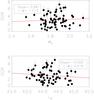 |
Fig. 6 Dwarf-to-giant ratio versus σV (upper panel) and LX (lower panel), with superimposed the least-squares fit. |
Again, there is a hint for less massive clusters (as traced by their X-ray luminosity) hosting a larger number of dwarf galaxies with respect to massive galaxies, but only if excluding the clusters where the DGR shows larger errors. If including the whole cluster sample, instead, both the relation with the X-ray luminosity and the relation with the velocity dispersion are not significant. In fact, the Spearman correlation test confirms that there is no correlation at all between the DGR ratio and the mass of the cluster.
4.2. LF of different subsamples
Here we consider various subsamples of clusters for which we construct the LF. First, we analyzed the LF of two subsamples characterized by extreme values of X-ray luminosity and velocity dispersion. We select the ten clusters with the highest (lowest) X-ray luminosity and the ten clusters with the highest (lowest) velocity dispersion.
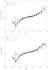 |
Fig. 7 Composite LF of galaxies belonging to the ten clusters with highest (and lowest) X-ray luminosities in the upper panel, and to the ten clusters with the highest (and lowest) velocity dispersions in the lower panel. The fits are drawn with a continuous line for the highest X-ray luminosity (velocity dispersion) samples, and with a dashed line for the lowest X-ray luminosity (velocity dispersion). |
In Fig. 7 we show the composite LF (i.e. the LF obtained from the single LFs by summing all contributions after having normalized them to have the same number of objects above a certain magnitude, see Sect. 5 for our own definition of composite LF) for these subsamples of clusters: in the upper panels WINGS clusters are subdivided according to their X-ray luminosity (taken from Ebeling et al. 1996, 1998, 2000), while in the lower panels they are separated on the basis of their velocity dispersion. In both figures, the filled symbols represent the LF for the sample with highest X-ray luminosity (velocity dispersion), while open symbols refer to those with the lowest X-ray luminosity (velocity dispersion). To better compare the two samples, they have been normalized so that they possess the same number of galaxies brighter than MV = −19. Superimposed are the two fits (in continuous and dashed, respectively, for the two subsamples) that we obtained leaving free all parameters of the double Schechter function. In order not to be biased by low statistics, we only fit points where the global contribution comes from at least five clusters. For this reason, the bins brighter than MV = −23 never contribute to the fit, and clusters with the smallest values of LX and σV have been fitted up to MV = −22.
The central part of the LF is very similar in the two subsamples, indicating that differences, if any, arise at the two extremes of the distributions. More massive clusters have a brighter characteristic magnitude and a steeper slope in the bright regime, with respect to clusters with smaller masses (see Hansen et al. 2005 and Croton et al. 2005 for similar results derived from local densities). The slope in the faint end part of the LF is −2.4 ± 0.1 and −2.5 ± 0.4 in the two subsamples, respectively, when looking at the trends with the X-ray luminosity, while it turns out to be −2.6 ± 0.4 and −2.1 ± 0.3, respectively, when dividing the samples according to their velocity dispersion. Therefore, given the uncertainties, we can conclude that the two shapes of the LF are very similar in both cases, confirming the results found in previous sections.
5. Composite luminosity function
The lack of any significant relation between the single cluster LFs and the overall cluster properties, led us to put more stringent constraint on our result by constructing the so-called composite LF. We calculated it by summing all the clusters LF after having normalized them in order to have the same number of objects brighter than MV = −19. To construct the LF, we follow a modified version of the formulation given by (Colless 1989; Popesso et al. 2006). The number of galaxies Nj in the final LF in the absolute magnitude jth bin is therefore calculated as  (5)where Nc,0 is the total number of galaxies brighter than MV = −19, mj is the number of clusters contributing to the jth bin, Ni,j is the number of galaxies in the jth bin coming from the ith cluster, and Ni,0 is the number of galaxies in the ith cluster brighter than MV = −19. Here we use
  instead of mj, as in the original formalism by Colless (1989) to end up with a LF representative of the average cluster. In fact, if we suppose that we have an ideal situation of mj = n identical clusters with Ni0 = Nnorm and Ni,j = Nj, we find
  (6)using the original formalism of Popesso et al. (2006) and substituting Eq. (6) in it we can see, after simple algebra, that Ncj = Nj × n; therefore in the original form, the LF results in n times the single LF, which is not a “true” LF. We avoid this by dividing the original expression by the factor mj, which is the number of clusters used in each bin. The errors on the single bin are derived as the squared root of the sum of the single variances divided by the number of clusters contributing to the given bin.
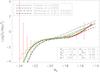 |
Fig. 8 Composite LF of WINGS galaxies. Superimposed are the double Schechter fits obtained having imposed the bright end slope αf = −1.10: red for the population of galaxies, green for the population of galaxies and unknown. The two insets in the lower right corner are the values of the fit. The black lines are fits taken from the literature (see the top left inset). |
Figure 8 shows the derived distribution for the sample of WINGS galaxies. The two fits obtained for the sample of galaxies (plus galaxies unknown) and the secondary sample of all objects (i.e. galaxies and unknown, without the sources classified as stars) are shown in red and green. While the two fits are coincident in the bright part, soon after the central plateau the mixed distribution starts rising, while the pure galaxy population remains flatter. In particular in the bright part the LF is well constrained and does not depend on the objects’ classification. At low luminosities where the classification of objects becomes more difficult, i.e. the galaxies/unknown separation is a critical issue, the LF varies in the two subsamples (as expected).
In particular, the best fit to our LF, after having fixed the bright end slope, as we did for the single LFs, gives MV,b = −21.40, MV,f = −16.24, and αf = −2.63 when we consider the galaxy population, while in the faint end we find MV,f = −16.94, and αf = −2.10 when including the unknown objects. In the plot we also superimpose the LF fit derived by Popesso et al. (2006) and Barkhouse et al. (2007), rescaled to match the bright part of the LF.
When we consider the sample of galaxies (plus galaxies unknown) our LF (and consequently its fit) is slightly different from those given in literature, even if still compatible. We find a steeper rising in the faint end regime and a more pronounced central plateau. If we include in our sample all unknown objects, instead, we find a better agreement, with a flatter slope and a brighter characteristic magnitude in the faint end part of the LF. However, the literature fits present a still higher number of low-luminosity objects, probably suggesting that the contribution of spurious classifications in the SDSS samples is not negligible and that our WINGS sample of galaxies (plus unknown galaxies) is a good tracer of the population of cluster galaxies at least in the range of magnitudes we are using.
5.1. LF of galaxies with different morphologies
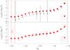 |
Fig. 9 Composite LF of galaxies classified as early-type (purple dots) and late-type (black diamonds) in the upper panel, while in the lower panel there are ellipticals (red dots) and S0 (red triangles). |
One of the main characteristics of clusters is the morphological mix of its galaxies. To test any dependence of the LF on morphology, we constructed the LF of galaxies according to their morphology.
Figure 9 shows the LFs of early-type galaxies (in red dots) and late-type galaxies (in black diamonds). In the bottom panel, we show the LF for ellipticals (red dots) and S0 (red triangles) galaxies. As already noted in Vulcani et al. (2011), the population of early-type galaxies is always predominant over the contribution of the late-type galaxies. The two shapes of the LF are different; the late-type galaxies show a flatter central plateau and a rapid decline at both bright and faint luminosities. As for the contribution of ellipticals and S0s, we show in Fig. 9 (lower panel) that the two populations have almost the same trend along the whole LF. However, at bright luminosities ellipticals outnumber S0s, while in the central plateau S0s seem to give a larger contribution (see also Vulcani et al. 2011 for the same conclusions about the mass functions).
This trend is partially at odds with the findings of Popesso et al. (2006), whose results demonstrated evidence for a large fraction of early-types in the faint end regime. However, their classification was mainly based on galaxy colours.
The analysis by Popesso et al. (2006) also shows a predominance of late-type dwarfs when moving towards the external regions of clusters. Unfortunately, we can not yet confirm this result at our redshifts, where clusters need larger CCDs to reach the r200 limit. However, our classification is based on morphological criteria, and not on the galaxy colours.
6. Spectroscopic luminosity function
Given the high spectroscopic coverage of our cluster sample, we finally calculated the spectroscopic LF. As previously done in other works (Vulcani et al. 2011), we decided here to consider only those clusters that have a spectroscopic completeness larger than 50%, i.e. 21 out of 48 clusters. The sample is made of 2009 galaxies that are cluster members.
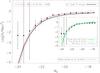 |
Fig. 10 Spectroscopic LF of WINGS cluster members. The single Schechter fit to the SLF is drawn in red, while black lines represent the fit to the photometric LF (continuous line), and the Schechter function obtained using the median values of the whole sample (dotted line). In the inset we compare our SLF with those by Rines & Geller (2008) for Virgo and A2199, and by Agulli et al. (2014) for A85. |
Figure 10 shows the spectroscopic LF (SLF) of the sample, after the correction made using both the spectroscopic and the photometric completeness, as described in Moretti et al. (2014), Sect. 6.3. The LF is obviously less deep than the photometric LF, and we decided to keep only points reaching –17.5 in V band absolute magnitude, as in this magnitude bin 17/21 clusters contribute to the galaxy population. The best fit of a single-Schechter function is superimposed to the points in a red dashed line (the values of the fit are given in the top left label). We also show the best fit of the photometric LF, normalized to the same constant (dotted line) and the fit obtained imposing the mode values of the entire sample (continuous line).
The SLF fit is very similar to the best fit of the photometric CLF, being  for the two fits, respectively. The mode of the global LF, when considering the population of galaxies corrected for the fraction of unknown that could be considered as galaxies, is
  . Our spectroscopic and photometric LFs are therefore in agreement, even if this can only be probed in the bright part of the LF.
Previous studies based on samples of spectroscopically confirmed cluster members found slightly steeper slopes for the Schechter fit: De Propris et al. (2003) analyzing 2dFGRS data in the bJ band gives α = −1.28, while Christlein & Zabludoff (2003) using R band data in six clusters estimated α = −1.21. Their magnitude limits extends from 3 to 7 mag below M∗, and it is therefore only marginally comparable with our observational range. In fact, their slope is derived using magnitudes where we do expect to find an upturn, but it is less pronounced than the slope we find using the photometric sample. It is interesting to compare our SLF with the results found in the recent works by Rines & Geller (2008) and Agulli et al. (2014) in which they derive the spectroscopic LF for Abell 2199, Virgo and Abell 85, respectively, reaching very faint magnitudes. In particular, we obtain good agreement of our SLF with the corresponding bright part of all SLFs, i.e. in the region where we possess spectroscopic information. In the faint end regime, we find a slightly shallower slope (–0.98 to be compared with –1.28 and –1.13 for Virgo and A2199, and with –1.58 found in A85).
7. Conclusions
We studied the LF in a sample of WINGS clusters up to 0.5 × r200. This allows us to evaluate the cluster LF in the same physical region in terms of radial coverage. Thanks to the work by Berta et al. (2006), based on observations made with our own observational setup, we were able to statistically subtract stars and background detections, and we found that a fit with a single Schechter function is not able to reproduce the entire range of the luminosity distribution. We therefore moved to the widely used approach of fitting a double Schechter function to our LFs.
We addressed the still unsolved question regarding the universality of the LF. We find that a large spread exists among values for single clusters, and the agreement with other studies is satisfying only when comparing the bright part of the LF, while discrepancies arise in the faint end. The fitted values for a single cluster do not depend on the global characteristics of the cluster itself, such as the X-ray luminosity or cluster velocity dispersion, which are, however, quantities derived for the global cluster (while the LF covers only the internal region). We find that in the LFs for extreme subsamples of galaxies, i.e. those showing the highest (and lowest) values of LX and σV, the overall shape of the two distributions is preserved. In addition, the DGR does not depend on cluster’s masses (as derived from the same proxies).
We constructed the composite LF by stacking all the LFs. This approach allows to reduce the errors on single cluster LF, having a much larger statistics in each LF bin. This LF is in excellent agreement with the results previously found for the bright part of the LF in other studies, while it shows a slightly steeper trend in the faint region. This steeper slope is somewhat compensated by the presence of a fainter characteristic magnitude, which leads to a more pronounced central plateau. If we include in the data detections belonging to the unknown class, we recover the faint end slope. We conclude that a careful object classification, possible only in dedicated survey such as ours, is the only way we have to discriminate which one of the two slopes is more probable. In addition, we point out that our LF is in good agreement with the recent findings by Agulli et al. (2014), who derived a spectroscopic LF down to Mr ~ − 16.0 for a cluster belonging to our sample.
We also used the morphological classification given by MORPHOT to derive the LFs of galaxies with different morphologies, up to the limit where the morphological classification was available for at least half of the photometric sample. We find that early-type galaxies dominate the LF over the entire magnitude range. Among early-type galaxies we find that ellipticals slightly outnumber S0s in the bright end, while the S0 fraction seems to increase in the central plateau.
Finally, we used a restricted sample of galaxies for which we have the spectroscopic membership confirmation to derive a clean LF. We obtained the LF only for the 21 clusters where the spectroscopic completeness is larger than 50%. Even though this LF is not as deep as the photometric LF (as expected), in the bright end we can confirm the values that we found from the photometric LF.
Our study indicates that the faint end LF slope might have been overestimated in the past, thus leading to a LF that is steeper than the real LF. This aspect needs to be assessed to link the presence of dwarfs to the cosmological predictions and/or to the higher redshift results (in which their mere presence is still debated; see Harsono & De Propris 2009; and Crawford et al. 2009, for different results). They seem to be equally divided into early and late morphologies, and among the early types they are again equally divided into ellipticals and S0s. When looking at the overall composition of the LF, instead, we find mainly S0 in the central plateau, and mainly ellipticals in the bright part of the LF. This could be the sign that between high and low redshift small S0s form by merging of small late types. However, deeper studies of local clusters by Trentham & Tully (2002), Hilker et al. (2003), Misgeld et al. (2009) demonstrated that the faint LF is much flatter than the results emerging from pure photometric studies (even if they looked for early-type galaxies), thus posing a dramatic challenge to the theoretical predictions by Moore et al. (1999), Jenkins et al. (2001) of a steep slope α = −2.0.
Online material
Schechter function parameters.
 |
Fig. A.1 LF for the cluster A85: the black continuous line is the original LF, the dashed line is the same LF corrected for completeness. The vertical line shows the magnitude limit (different for each cluster) at which the completeness is 90%. In red and green we show the LF of the two subsamples of galaxies and galaxies and unknown object, respectively. These two last distributions have been corrected for field contamination (whose number counts are shown in the inset). Superimposed on the red LF is the best fit that we obtained using a single Schechter function (left panel) and a double Schechter function (right panel). In the bottom right insets we give the relative parameters. |
 |
Fig. A.1 continued. |
 |
Fig. A.1 continued. |
 |
Fig. A.1 continued. |
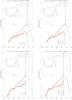 |
Fig. A.1 continued. |
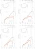 |
Fig. A.1 continued. |
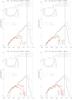 |
Fig. A.1 continued. |
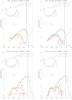 |
Fig. A.1 continued. |
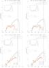 |
Fig. A.1 continued. |
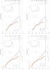 |
Fig. A.1 continued. |
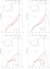 |
Fig. A.1 continued. |
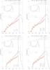 |
Fig. A.1 continued. |
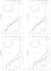 |
Fig. A.1 continued. |
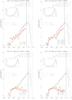 |
Fig. A.1 continued. |
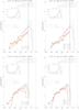 |
Fig. A.1 continued. |
 |
Fig. A.1 continued. |
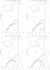 |
Fig. A.1 continued. |
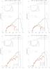 |
Fig. A.1 continued. |
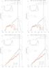 |
Fig. A.1 continued. |
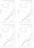 |
Fig. A.1 continued. |
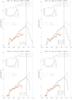 |
Fig. A.1 continued. |
 |
Fig. A.1 continued. |
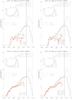 |
Fig. A.1 continued. |
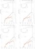 |
Fig. A.1 continued. |
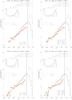 |
Fig. A.1 continued. |
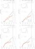 |
Fig. A.1 continued. |
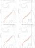 |
Fig. A.1 continued. |
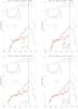 |
Fig. A.1 continued. |
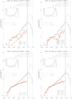 |
Fig. A.1 continued. |
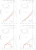 |
Fig. A.1 continued. |
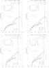 |
Fig. A.1 continued. |
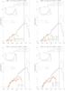 |
Fig. A.1 continued. |
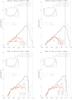 |
Fig. A.1 continued. |
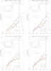 |
Fig. A.1 continued. |
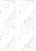 |
Fig. A.1 continued. |
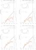 |
Fig. A.1 continued. |
Acknowledgments
We acknowledge the financial contribution from PRIN/INAF2014 “Galaxy evolution from cluster cores to filaments”. B.V. acknowledges the World Premier International Research Center Initiative (WPI), MEXT, Japan and the Kakenhi Grant-in-Aid for Young Scientists (B)(26870140) from the Japan Society for the Promotion of Science (JSPS). We thank the anonymous referee whose comments greatly improved the paper.
References
- Abazajian, K. N., Adelman-McCarthy, J. K., Agüeros, M. A., et al. 2009, ApJS, 182, 543 [NASA ADS] [CrossRef] [Google Scholar]
- Agulli, I., Aguerri, J. A. L., Sánchez-Janssen, R., et al. 2014, MNRAS, 444, L34 [NASA ADS] [CrossRef] [Google Scholar]
- Bai, L., Rieke, G. H., Rieke, M. J., et al. 2006, ApJ, 639, 827 [NASA ADS] [CrossRef] [Google Scholar]
- Barkhouse, W. A., Yee, H. K. C., & López-Cruz, O. 2007, ApJ, 671, 1471 [NASA ADS] [CrossRef] [Google Scholar]
- Bautz, L. P., & Morgan, W. W. 1970, ApJ, 162, L149 [NASA ADS] [CrossRef] [Google Scholar]
- Berta, S., Rubele, S., Franceschini, A., et al. 2006, A&A, 451, 881 [NASA ADS] [CrossRef] [EDP Sciences] [Google Scholar]
- Bertin, E., & Arnouts, S. 1996, A&AS, 117, 393 [NASA ADS] [CrossRef] [EDP Sciences] [Google Scholar]
- Blanton, M. R., Lupton, R. H., Schlegel, D. J., et al. 2005, ApJ, 631, 208 [NASA ADS] [CrossRef] [Google Scholar]
- Boselli, A., Boissier, S., Cortese, L., & Gavazzi, G. 2008, ApJ, 674, 742 [NASA ADS] [CrossRef] [Google Scholar]
- Boué, G., Adami, C., Durret, F., Mamon, G. A., & Cayatte, V. 2008, A&A, 479, 335 [NASA ADS] [CrossRef] [EDP Sciences] [Google Scholar]
- Bruzual, G., & Charlot, S. 2003, MNRAS, 344, 35 [Google Scholar]
- Calvi, R., Poggianti, B. M., Fasano, G., & Vulcani, B. 2011a, MNRAS, L354 [Google Scholar]
- Calvi, R., Poggianti, B. M., & Vulcani, B. 2011b, MNRAS, 416, 727 [NASA ADS] [Google Scholar]
- Cava, A., Bettoni, D., Poggianti, B. M., et al. 2009, A&A, 495, 707 [NASA ADS] [CrossRef] [EDP Sciences] [Google Scholar]
- Christlein, D., & Zabludoff, A. I. 2003, ApJ, 591, 764 [NASA ADS] [CrossRef] [Google Scholar]
- Colless, M. 1989, MNRAS, 237, 799 [NASA ADS] [CrossRef] [Google Scholar]
- Cortese, L., Gavazzi, G., Boselli, A., et al. 2003, A&A, 410, L25 [NASA ADS] [CrossRef] [EDP Sciences] [Google Scholar]
- Crawford, S. M., Bershady, M. A., & Hoessel, J. G. 2009, ApJ, 690, 1158 [NASA ADS] [CrossRef] [Google Scholar]
- Croton, D. J., Farrar, G. R., Norberg, P., et al. 2005, MNRAS, 356, 1155 [NASA ADS] [CrossRef] [Google Scholar]
- De Propris, R., Eisenhardt, P. R., Stanford, S. A., & Dickinson, M. 1998, ApJ, 503, L45 [NASA ADS] [CrossRef] [Google Scholar]
- De Propris, R., Colless, M., Driver, S. P., et al. 2003, MNRAS, 342, 725 [NASA ADS] [CrossRef] [Google Scholar]
- Deady, J. H., Boyce, P. J., Phillipps, S., et al. 2002, MNRAS, 336, 851 [NASA ADS] [CrossRef] [Google Scholar]
- Dressler, A. 1978, ApJ, 223, 765 [NASA ADS] [CrossRef] [Google Scholar]
- Driver, S., & De Propris, R. 2003, Ap&SS, 285, 175 [NASA ADS] [CrossRef] [Google Scholar]
- Driver, S. P., Phillipps, S., Davies, J. I., Morgan, I., & Disney, M. J. 1994, MNRAS, 268, 393 [NASA ADS] [CrossRef] [Google Scholar]
- Driver, S. P., Liske, J., Cross, N. J. G., De Propris, R., & Allen, P. D. 2005, MNRAS, 360, 81 [NASA ADS] [CrossRef] [Google Scholar]
- Ebeling, H., Voges, W., Bohringer, H., et al. 1996, MNRAS, 281, 799 [NASA ADS] [CrossRef] [Google Scholar]
- Ebeling, H., Edge, A. C., Bohringer, H., et al. 1998, MNRAS, 301, 881 [NASA ADS] [CrossRef] [Google Scholar]
- Ebeling, H., Edge, A. C., Allen, S. W., et al. 2000, MNRAS, 318, 333 [NASA ADS] [CrossRef] [Google Scholar]
- Fasano, G., Marmo, C., Varela, J., et al. 2006, A&A, 445, 805 [NASA ADS] [CrossRef] [EDP Sciences] [Google Scholar]
- Fasano, G., Bettoni, D., Ascaso, B., et al. 2010, MNRAS, 404, 1490 [NASA ADS] [Google Scholar]
- Fasano, G., Vanzella, E., Dressler, A., et al. 2012, MNRAS, 420, 926 [NASA ADS] [CrossRef] [Google Scholar]
- Ferguson, H. C. 1989, AJ, 98, 367 [Google Scholar]
- Finn, R. A., Zaritsky, D., McCarthy, Jr., D. W., et al. 2005, ApJ, 630, 206 [NASA ADS] [CrossRef] [Google Scholar]
- Fritz, J., Poggianti, B. M., Bettoni, D., et al. 2007, A&A, 470, 137 [NASA ADS] [CrossRef] [EDP Sciences] [Google Scholar]
- Fritz, J., Poggianti, B. M., Cava, A., et al. 2010, A&A, 526, A45 [Google Scholar]
- Fritz, J., Poggianti, B. M., Cava, A., et al. 2014, A&A, 566, A32 [NASA ADS] [CrossRef] [EDP Sciences] [Google Scholar]
- Garilli, B., Maccagni, D., & Andreon, S. 1999, A&A, 342, 408 [NASA ADS] [Google Scholar]
- González, R. E., Lares, M., Lambas, D. G., & Valotto, C. 2006, A&A, 445, 51 [NASA ADS] [CrossRef] [EDP Sciences] [Google Scholar]
- Goto, T., Okamura, S., McKay, T. A., et al. 2002, PASJ, 54, 515 [NASA ADS] [CrossRef] [Google Scholar]
- Hansen, S. M., McKay, T. A., Wechsler, R. H., et al. 2005, ApJ, 633, 122 [NASA ADS] [CrossRef] [Google Scholar]
- Harsono, D., & De Propris, R. 2009, AJ, 137, 3091 [NASA ADS] [CrossRef] [Google Scholar]
- Hilker, M., Mieske, S., & Infante, L. 2003, A&A, 397, L9 [NASA ADS] [CrossRef] [EDP Sciences] [Google Scholar]
- Jenkins, A., Frenk, C. S., White, S. D. M., et al. 2001, MNRAS, 321, 372 [NASA ADS] [CrossRef] [MathSciNet] [Google Scholar]
- Liske, J., Lemon, D. J., Driver, S. P., Cross, N. J. G., & Couch, W. J. 2003, MNRAS, 344, 307 [NASA ADS] [CrossRef] [Google Scholar]
- Lopez-Cruz, O., Yee, H. K. C., Brown, J. P., Jones, C., & Forman, W. 1997, ApJ, 475, L97 [NASA ADS] [CrossRef] [Google Scholar]
- López-Cruz, O., Barkhouse, W. A., & Yee, H. K. C. 2004, ApJ, 614, 679 [NASA ADS] [CrossRef] [Google Scholar]
- Lugger, P. M. 1986, ApJ, 303, 535 [NASA ADS] [CrossRef] [Google Scholar]
- Madgwick, D. S., Lahav, O., Baldry, I. K., et al. 2002, MNRAS, 333, 133 [NASA ADS] [CrossRef] [Google Scholar]
- Misgeld, I., Hilker, M., & Mieske, S. 2009, A&A, 496, 683 [NASA ADS] [CrossRef] [EDP Sciences] [Google Scholar]
- Mobasher, B., Colless, M., Carter, D., et al. 2003, ApJ, 587, 605 [NASA ADS] [CrossRef] [Google Scholar]
- Moore, B., Ghigna, S., Governato, F., et al. 1999, ApJ, 524, L19 [Google Scholar]
- Moretti, A., Poggianti, B. M., Fasano, G., et al. 2014, A&A, 564, A138 [NASA ADS] [CrossRef] [EDP Sciences] [Google Scholar]
- Omizzolo, A., Fasano, G., Reverte Paya, D., et al. 2014, A&A, 561, A111 [NASA ADS] [CrossRef] [EDP Sciences] [Google Scholar]
- Paolillo, M., Andreon, S., Longo, G., et al. 2001, A&A, 367, 59 [Google Scholar]
- Penny, S. J., Conselice, C. J., de Rijcke, S., et al. 2011, MNRAS, 410, 1076 [NASA ADS] [CrossRef] [Google Scholar]
- Poggianti, B. M. 1997, A&AS, 122, 399 [NASA ADS] [CrossRef] [EDP Sciences] [Google Scholar]
- Poggianti, B. M., Bridges, T. J., Mobasher, B., et al. 2001, ApJ, 562, 689 [NASA ADS] [CrossRef] [Google Scholar]
- Poggianti, B. M., von der Linden, A., De Lucia, G., et al. 2006, ApJ, 642, 188 [NASA ADS] [CrossRef] [Google Scholar]
- Popesso, P., Biviano, A., Böhringer, H., & Romaniello, M. 2006, A&A, 445, 29 [NASA ADS] [CrossRef] [EDP Sciences] [Google Scholar]
- Rauzy, S., Adami, C., & Mazure, A. 1998, A&A, 337, 31 [NASA ADS] [Google Scholar]
- Rines, K., & Geller, M. J. 2008, AJ, 135, 1837 [NASA ADS] [CrossRef] [Google Scholar]
- Schechter, P. 1976, ApJ, 203, 297 [Google Scholar]
- Trentham, N., & Hodgkin, S. 2002, MNRAS, 333, 423 [NASA ADS] [CrossRef] [Google Scholar]
- Trentham, N., & Tully, R. B. 2002, MNRAS, 335, 712 [NASA ADS] [CrossRef] [Google Scholar]
- Valentinuzzi, T., Woods, D., Fasano, G., et al. 2009, A&A, 501, 851 [NASA ADS] [CrossRef] [EDP Sciences] [Google Scholar]
- Valotto, C. A., Nicotra, M. A., Muriel, H., & Lambas, D. G. 1997, ApJ, 479, 90 [NASA ADS] [CrossRef] [Google Scholar]
- Varela, J., D’Onofrio, M., Marmo, C., et al. 2009, A&A, 497, 667 [NASA ADS] [CrossRef] [EDP Sciences] [Google Scholar]
- Vulcani, B., Poggianti, B. M., Aragón-Salamanca, A., et al. 2011, MNRAS, 412, 246 [NASA ADS] [CrossRef] [Google Scholar]
- Yagi, M., Kashikawa, N., Sekiguchi, M., et al. 2002, AJ, 123, 87 [NASA ADS] [CrossRef] [Google Scholar]
All Tables
All Figures
|
Fig. 1 LF for the cluster A85: the black continuous line is the original LF, the dashed line is the same LF corrected for completeness. The vertical line shows the magnitude limit (different for each cluster) at which the completeness is 90%. In red and green we show the LF of the two subsamples of galaxies and galaxies and unknown object, respectively. These two last distributions have been corrected for field contamination (whose number counts are shown in the inset). Superimposed on the red LF is the best fit that we obtained using a single Schechter function (left panel) and a double Schechter function (right panel). In the bottom right insets we give the relative parameters. |
| In the text | |
|
Fig. 2 Distribution of |
| In the text | |
|
Fig. 3 Comparison with literature data, homogenized to the same photometric band and cosmological parameters. The squared point refers to the WINGS median values, the circle is the mode, while the triangle is the weighted mean. Errors are the mean errors in the derived parameters. |
| In the text | |
|
Fig. 4 Comparison with literature data, homogenized to the same photometric band and cosmological parameters. Squared point refer to the WINGS median values of the galaxies (including the unknown galaxies) subsample, the triangle to the subsample all objects of galaxies and unknown sources, excluding stars. When fixing the αb the |
| In the text | |
|
Fig. 5 Variation of αf (left panels) and MV (right panels) with σv (upper panel) and LX (lower panel), with superimposed the least-squares fit. |
| In the text | |
|
Fig. 6 Dwarf-to-giant ratio versus σV (upper panel) and LX (lower panel), with superimposed the least-squares fit. |
| In the text | |
|
Fig. 7 Composite LF of galaxies belonging to the ten clusters with highest (and lowest) X-ray luminosities in the upper panel, and to the ten clusters with the highest (and lowest) velocity dispersions in the lower panel. The fits are drawn with a continuous line for the highest X-ray luminosity (velocity dispersion) samples, and with a dashed line for the lowest X-ray luminosity (velocity dispersion). |
| In the text | |
|
Fig. 8 Composite LF of WINGS galaxies. Superimposed are the double Schechter fits obtained having imposed the bright end slope αf = −1.10: red for the population of galaxies, green for the population of galaxies and unknown. The two insets in the lower right corner are the values of the fit. The black lines are fits taken from the literature (see the top left inset). |
| In the text | |
|
Fig. 9 Composite LF of galaxies classified as early-type (purple dots) and late-type (black diamonds) in the upper panel, while in the lower panel there are ellipticals (red dots) and S0 (red triangles). |
| In the text | |
|
Fig. 10 Spectroscopic LF of WINGS cluster members. The single Schechter fit to the SLF is drawn in red, while black lines represent the fit to the photometric LF (continuous line), and the Schechter function obtained using the median values of the whole sample (dotted line). In the inset we compare our SLF with those by Rines & Geller (2008) for Virgo and A2199, and by Agulli et al. (2014) for A85. |
| In the text | |
|
Fig. A.1 LF for the cluster A85: the black continuous line is the original LF, the dashed line is the same LF corrected for completeness. The vertical line shows the magnitude limit (different for each cluster) at which the completeness is 90%. In red and green we show the LF of the two subsamples of galaxies and galaxies and unknown object, respectively. These two last distributions have been corrected for field contamination (whose number counts are shown in the inset). Superimposed on the red LF is the best fit that we obtained using a single Schechter function (left panel) and a double Schechter function (right panel). In the bottom right insets we give the relative parameters. |
| In the text | |
|
Fig. A.1 continued. |
| In the text | |
|
Fig. A.1 continued. |
| In the text | |
|
Fig. A.1 continued. |
| In the text | |
|
Fig. A.1 continued. |
| In the text | |
|
Fig. A.1 continued. |
| In the text | |
|
Fig. A.1 continued. |
| In the text | |
|
Fig. A.1 continued. |
| In the text | |
|
Fig. A.1 continued. |
| In the text | |
|
Fig. A.1 continued. |
| In the text | |
|
Fig. A.1 continued. |
| In the text | |
|
Fig. A.1 continued. |
| In the text | |
|
Fig. A.1 continued. |
| In the text | |
|
Fig. A.1 continued. |
| In the text | |
|
Fig. A.1 continued. |
| In the text | |
|
Fig. A.1 continued. |
| In the text | |
|
Fig. A.1 continued. |
| In the text | |
|
Fig. A.1 continued. |
| In the text | |
|
Fig. A.1 continued. |
| In the text | |
|
Fig. A.1 continued. |
| In the text | |
|
Fig. A.1 continued. |
| In the text | |
|
Fig. A.1 continued. |
| In the text | |
|
Fig. A.1 continued. |
| In the text | |
|
Fig. A.1 continued. |
| In the text | |
|
Fig. A.1 continued. |
| In the text | |
|
Fig. A.1 continued. |
| In the text | |
|
Fig. A.1 continued. |
| In the text | |
|
Fig. A.1 continued. |
| In the text | |
|
Fig. A.1 continued. |
| In the text | |
|
Fig. A.1 continued. |
| In the text | |
|
Fig. A.1 continued. |
| In the text | |
|
Fig. A.1 continued. |
| In the text | |
|
Fig. A.1 continued. |
| In the text | |
|
Fig. A.1 continued. |
| In the text | |
|
Fig. A.1 continued. |
| In the text | |
|
Fig. A.1 continued. |
| In the text | |
Current usage metrics show cumulative count of Article Views (full-text article views including HTML views, PDF and ePub downloads, according to the available data) and Abstracts Views on Vision4Press platform.
Data correspond to usage on the plateform after 2015. The current usage metrics is available 48-96 hours after online publication and is updated daily on week days.
Initial download of the metrics may take a while.