| Issue |
A&A
Volume 580, August 2015
|
|
|---|---|---|
| Article Number | A104 | |
| Number of page(s) | 11 | |
| Section | Extragalactic astronomy | |
| DOI | https://doi.org/10.1051/0004-6361/201525649 | |
| Published online | 10 August 2015 | |
Nine years of multi-frequency monitoring of the blazar PKS 0048-097: spectral and temporal variability
1 Insitute of Nuclear Physics, Polish Academy of Sciences, ul. Radzikowskiego 152, 31-342 Kraków, Poland
e-mail: alicja.wierzcholska@ifj.edu.pl
2 Landessternwarte, Universität Heidelberg, Königstuhl 12, 69117 Heidelberg, Germany
Received: 12 January 2015
Accepted: 4 June 2015
Context. Blazars are highly variable, radio-loud active galactic nuclei with jets oriented at a small angle to the line of sight. The observed emission of these sources covers the whole electromagnetic spectrum from radio frequencies up to the high or even very high energy gamma-ray range. To understand the complex physics of these objects, multi-wavelength observations and studies on the variability and correlations between different wavelengths are therefore essential.
Aims. The long-term multi-frequency observations of PKS 0048−097 are analysed here to investigate its spectral and temporal features. The studies includes nine years of observations of the blazar, which is well studied in the optical and radio domain, but not in the other frequencies.
Methods. Multi-wavelength data collected with OVRO, KAIT, Catalina, Swift/UVOT, Swift/XRT, and Fermi/LAT were studied.
Results. The performed analysis revealed strong variability in all wavelengths that is most clearly manifested in the X-ray range. The correlation studies do not exhibit any relation between different wavelengths, except for the very strong positive correlation between the optical emission in V and R bands.
Key words: radiation mechanisms: non-thermal / galaxies: active / BL Lacertae objects: general / galaxies: jets
© ESO, 2015
1. Introduction
Blazars constitute an extreme class of radio-loud active galactic nuclei (AGN), which are characterized by a relativistic jet that is pointed at small angles to the observer (e.g. Begelman et al. 1984), and polarized and highly variable non-thermal continuum emission extending through the entire electromagnetic spectrum, from radio to X-rays and, or even, up to high and very high energy γ-rays (e.g. Gupta et al. 2008; Wagner 2009; Vercellone et al. 2011; Giommi et al. 2012; Abramowski et al. 2013, 2014b). The rapid variability of blazars is visible at different wavelengths on different timescales down to hours or even shorter (e.g. Wagner & Witzel 1995; Aharonian et al. 2007; Saito et al. 2013).
This class of objects includes the flat-spectrum radio-loud quasars (FSRQs) as well as the BL Lacertae type (BL Lac) objects. For FSRQs the presence of prominent broad and narrow emission lines are characteristic, while the featureless continuum emission in the optical band is attributed to the BL Lac type objects (e.g. Urry & Padovani 1995). The spectral energy distribution (SED), in νFν representation, usually has a double-peaked structure that is generated by two emission components. The first bump located between the optical and X-ray regimes is described by the synchrotron radiation from the relativistic electrons in the jet. The second bump can be explained either by leptonic or by the hadronic scenarios. In the leptonic models the high-energy part of the SED, located in the hard X-ray-to-gamma-ray regime, is produced by the inverse-Compton (IC) emission of the same electron population, involving either the jet synchrotron photons as a seed for the IC scattering (synchrotron self-Compton model, SSC; e.g. Konigl 1981; Marscher & Gear 1985; Band & Grindlay 1985), or various photon fields originating outside of the jet (external-Compton models; e.g. Dermer et al. 1992; Sikora et al. 1994). Alternatively, the second bump can be explained in the framework of hadronic scenarios that are mostly initiated by the relativistic protons accelerated with the electrons (see e.g. Mannheim & Biermann 1992; Mücke et al. 2003; Böttcher 2007). The location of the low-energy peak in the SED subdivides blazars into three subclasses of high-, intermediate-, and low-energy peaked sources (HBLs, IBLs, and LBLs, respectively), depending on the position of their synchrotron peak frequencies (see e.g. Padovani & Giommi 1995; Fossati et al. 1998; Abdo et al. 2010a).
Parameters of the spectral analysis of Swift/XRT data.
PKS 0048−097 (RA2000: 00h50m41.317s, Dec2000: −09°29′05.21′′) is a BL Lac-type blazar (Plotkin et al. 2008) located at redshift z = 0.635 (Landoni et al. 2012), which is well studied in the optical and radio regime (e.g. Ross 1970; Carswell et al. 1973; Pica et al. 1988; Wills et al. 1992; Falomo 1996; Stickel et al. 1993; Sefako et al. 2001). The source was reported in the first (Abdo et al. 2010b) and second (Nolan et al. 2012) Fermi/LAT Catalogs and Fermi Bright Gamma-ray Source List (Abdo et al. 2009a), known as 1FGL, 2FGL, and 0FGL, respectively. No detection in the very high energy gamma-rays range has been reported, meaning that there is only an upper limit on flux provided by the H.E.S.S. Collaboration (Abramowski et al. 2014a). Abdo et al. (2010a) found the frequency of lower peak to be log νsyn = 14.3, which allows classifying the object as an IBL-type source.
For the first time, we present here the results of nine years of multi-wavelength observations of PKS 0048−097 covering the radio, optical, UV, X-ray, and high-energy gamma-ray wavelengths. The paper is organized as follows: Sect. 2 describes the multi-frequency observations of the source, Sect. 3 shows the behaviour of PKS 0048−097 in both the quiescence and flaring states and the spectral properties in GeV range. Section 4 discuss the multi-frequency correlations. The work is summarized in Sect. 5.
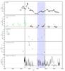 |
Fig. 1 Multi-wavelength light curve of PKS 0048−097. Panels from the top to the bottom show the radio observations from the OVRO telescope at 15 GHz; optical (KAIT and Catalina) monitoring in R and V band, Swift/UVOT data in V, B, U, UVW1, UVM2, and UVW2 filters, X-ray observations with Swift/XRT, and Fermi/LAT flux (E> 100 MeV). The horizontal dashed lines in all the panels represent the average flux for all observations presented here. In all the cases (excluding Fermi/LAT data) each point corresponds to one night of observations; for the case of Fermi/LAT monitoring data are binned in week-long intervals. In the Fermi/LAT light curve, flux upper limits are represented with grey points. The time periods corresponding to A and B flares are marked in grey, while the quiescence period Q is plotted in blue. |
2. Multi-wavelength data
2.1. Gamma-ray monitoring with Fermi/LAT
The LAT, on-board the Fermi satellite, is a pair-conversion detector that is sensitive to photons in the energy band from ~ 20 MeV to a few hundred GeV (Atwood et al. 2009). This primary mission instrument covers the full sky every three hours, and the data are available publicly on the mission web page1.
PKS 0048−097 is included in 2FGL (as well as in previous catalogues: 0FGL and 1FGL) as 2FGL 0050.6−0926 with an average flux between 100 MeV and 100 GeV of (3.85 ± 0.25) × 10-9 ph cm-2 s-1 and the spectral index of Γ2FGL = 2.14 ± 0.04. For comparison, the 1FGL reports an average flux in the same energy range of (4.50 ± 0.45) × 10-9 ph cm-2 s-1 and a spectral index of Γ1FGL = 2.19 ± 0.05, while the reported flux level in 0FGL is (7.2 ± 1.0) × 10-9 ph cm-2 s-1.
For this paper data collected between August 4, 2008 and July 1, 2014 were analysed using standard Fermi Science tools (version v9r33p0) with P7REP_SOURCE_V15_rev1 instrument response functions (IRFs). For the analysis the photons with a zenith angle < 105° were selected in the energy range of 100 MeV to 300 GeV. Events were selected in a 15° region of interest (ROI) centred on PKS 0048−097. The binned maximum-likelihood method (Mattox et al. 1996) was applied in the analysis. The Galactic diffuse background was modelled using the gll_iem_v05 map cube, and the extragalactic diffuse and residual instrument backgrounds were modelled jointly using the isotropic_iem_v02 template. All the sources from the Fermi/LAT Second Source Catalog (2FGL, Nolan et al. 2012) inside the ROI of PKS 0048−097 were modelled.
The long-term light curve binned in seven-day intervals is presented in Fig. 1.
Magnitudes for different epochs from Swift/UVOT data for V, B, U, UVW1, UVM2, and UVW2 filters.
2.2. X-ray observations with Swift
The Swift mission (Gehrels et al. 2004) is a multi-wavelength space observatory launched into orbit on November 20, 2004. The instrument is equipped with the following detectors: the Burst Alert Telescope (BAT, Barthelmy et al. 2005), the X-ray Telescope (XRT, Burrows et al. 2005), and the Ultraviolet/Optical Telescope (UVOT, Roming et al. 2005).
PKS 0048−097 was monitored with Swift/XRT in nine pointed observations (all in PC mode), resulting in total exposure of 32.1 ks. These data were analysed using version 6.15 of the HEASOFT package2. Data were recalibrated using the standard procedure xrtpipeline. All the observations were checked for the pile-up effect, which was found to be negligible. Spectral analysis was performed for data in the energy range of 0.3−10 keV with the latest version of the XSPEC package (version 12.8.2). All data were binned to have at least 30 counts per bin. Spectra are well fitted with a power-law function with a Galactic absorption value of NH = 3.22 × 1020 cm-2 (Kalberla et al. 2005) set as a frozen parameter. The power-law fit parameters are collected in Table 1.
The long-term light curve of the integrated flux in the energy range of 2.0−10 keV, presented in Fig. 1, shows the significant variability of the source. There are no significant changes in the spectral index for the period of observations (see Table 1).
2.3. UV observations with Swift
The UVOT instrument measures the UV and optical emission simultaneous to the X-ray telescope. The observations are taken in the UV and optical bands with central wavelengths of UVW2 (188 nm), UVM2 (217 nm), UVW1 (251 nm), U (345 nm), B (439 nm), and V (544 nm).
The instrumental magnitudes were calculated using uvotsource taking into account all photons from a circular region with radius 5′′. The background was determined from a circular region with radius 10′′ near the source region. The flux conversion factors used are provided by Poole et al. (2008). All UVOT data were corrected for the dust absorption using the reddening E(B−V) = 0.0274 mag (Schlafly & Finkbeiner 2011) and the ratios of the extinction to reddening, Aλ/E(B−V), for each filter (Giommi et al. 2006). All the measured magnitudes are collected in Table 2, while the Swift/UVOT light curve is presented in Fig. 1.
2.4. Optical monitoring with Catalina and with KAIT
PKS 0048−097 is one of the frequently monitored targets by the two optical instruments Catalina and KAIT, which observe the blazar in V and R bands, respectively. Both light curves were used in this paper.
The Catalina Survey (Drake et al. 2009) consists of the Catalina Sky Survey (CSS) and the Catalina Real-time Transient Survey (CRTS). Here only CSS data in V band are used, which are publicly available on the instrument web page3.
The second optical monitoring we present was obtained with The Katzman Automatic Imaging Telescope Gamma-Ray Burst KAIT (Li et al. 2000). KAIT is the third robotic telescope in the Berkeley Automatic Imaging Telescope (BAIT) program (Richmond et al. 1993; Treffers et al. 1995). The instrument monitors 163 AGNs with an average cadence of three days. Data points in the light curves in R band (Li et al. 2003) are produced through a pipeline described by Cohen et al. (2014) and available on the program web page4.
The host galaxy of PKS 0048−097 remains unresolved (Kotilainen et al. 1998), and because of this, the data were not corrected for the influence of the host. All optical magnitudes were corrected against the Galactic extinction based on the model by Schlegel et al. (1998) with the most recent recalibration by Schlafly & Finkbeiner (2011), using the correction factors of AV = 0.088 and AR = 0.069, for V and R band, respectively.
Fractional variability in different energy bands.
2.5. Radio observations with OVRO
The radio observations of PKS 0048−097 were carried out at 15 GHz with the Owens Valley Radio Observatory (OVRO), which is the 40 m telescope dedicated to observe Fermi/LAT targets (Richards et al. 2011). Data used in this analysis were collected between January 6, 2008 to May 8, 2014 and were downloaded from the programme website5.
3. Multi-wavelength behaviour and flaring activity of PKS 0048−097
Studies on multi-wavelength behaviour using simultaneous observations of the blazars, both in quiescence and flaring state, are crucial to understand the physics and nature of these objects. PKS 0048−097 is a highly variable source, significant flux changes are observed in all wavelengths (see Fig. 1).
3.1. Temporal and spectral variability of the blazar
To quantify the temporal variability that is observed in different wavelengths, the fractional variability amplitude is calculated using formula provided by Vaughan et al. (2003), 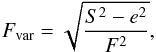 (1)where S2 is the variance, e2 is the mean square error, and F is the mean flux. The uncertainty of Fvar is calculated following the formula by Poutanen et al. (2008),
 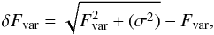 (2)with the error in the normalised excess variance σ given as (Vaughan et al. 2003)
 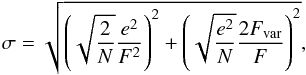 (3)where N is the number of data points in the light curve. The calculated values of Fvar for all the energy bands we analysed are collected in Table 3. Figure 3 shows changes of the Fvar values in different energy bands. During the whole monitoring period of the blazar, significant variability was revealed in the Fvar values. The lowest Fvar value is for the GeV observation, the highest for X-ray range, while for the other ranges the Fvar values are similar. We note that for Fermi/LAT data Fvar was only calculated for the flux points, and the upper limit points were omitted from the calculations.
It is important to mention that the values of Fvar are strongly dependent on the size of the time bins in the light curves. Smaller bins allow showing stronger flux variations, which in the case of larger time bins can be smoothed out and lead to lower Fvar values. Obviously, the time binning is limited by the characteristics of particular instruments. The second factor that influences the values of Fvar are the flux uncertainties. The uncertainties according to the definition are expected to be constant (or at least very close to constant), which in practice is not always true. For example, such a case is visible in the optical monitoring with Catalina (see Fig. 1), in which some measurements have much larger uncertainties than the others.
Figure 1 reveals the variable nature of the source. Nine years of this this long-term monitoring allow pointing out significant variability patterns that are observed in different wavelengths.
Radio variability
In the radio band the flux oscillates between 0.2 × 10⁻¹³ erg cm-2 s-1 and 3.6 × 10⁻¹³ erg cm-2 s-1. The highest mentioned value corresponds to about 2.4 Jy, the lowest to about 0.2 Jy. The highest flux level is observed during the period of MJD 54 762−MJD 54 998, while the lowest values are collected during the period of MJD 55 321−MJD 55 505. As mentioned before, PKS 0048−097 was a target of several previous radio monitorings. Long-term radio observations provided by the Michigan group6 during the period of 1970−2010 showed, for instance, that the flux changes at 14.5 GHz between 0.3−2.8 Jy, with the highest value archived in 1993. The second prominent outburst reported by the scientists is observed at the end of 2009 with an observed flux level of about 2.4 Jy. The second mentioned flare can correspond to the main outburst (MJD 54 900) visible in OVRO observations.
Optical variability
The optical monitoring with Catalina includes 100 months of observations, while the monitoring with KAIT includes about 54 months. The significant optical variability of the source is revealed in several flares that were observed both in R and V band. The strongest outburst took place between MJD 55 822 and MJD 55 951, and it shows flux changes in the range of about 3 × 10-11 erg cm-2 s-1 in V band (during this period PKS 0048−097 was not monitored with KAIT). Observations of the blazar with KAIT reveal a prominent outburst with 3.5 mag amplitude. We highlight here that this is the largest optical flare ever reported for this blazar. Previous studies that focused on the optical variability of PKS 0048−097 have also shown a significant outburst of 3 mag (Usher et al. 1974).
X-ray and UV variability
Nine pointing observations of PKS 0048−097 with Swift/UVOT and Swift/XRT also show changes in the flux. In the X-ray range the largest outburst was observed in June 2009. The highest flares observed with Swift/UVOT occurred in June 2009 and January 2012. The first flare is simultaneous with that of Swift/XRT, while the second optical-UV outburst is not correlated with the X-ray flux. No significant variability is observed in the Swift/XRT spectral index (see Fig. 2).
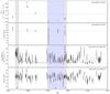 |
Fig. 2 Temporal and spectral variability of PKS 0048−097 observed with Swift/XRT and Fermi/LAT. The following panels present the X-ray temporal and spectral variability and the γ-ray temporal and spectral variability. For Swift/XRT observations one point correspond to one day of observations, while in the case of Fermi/LAT data one point is for weekly integrated observations. We plot the flux upper limits in the Fermi/LAT light curve with grey points. The time periods corresponding to A and B flares are marked in grey, while the quiescence period Q is shown in blue. |
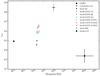 |
Fig. 3 Fractional variability vs. frequency for each observation regime. The numerical values can be found in Table 3. The colours for the data points are the same as in Fig. 1. |
GeV temporal and spectral variability
The gamma-ray monitoring of the blazar presented here includes more than five years of observations beginning from the mission start date. The observed flux in this energy range shows significant temporal variability. The variability is also observed for the spectral index in this wavelength. We note that in the GeV regime the observed emission is not very strong because the light curve (see Fig. 1) includes many of the flux upper limits points and the flux points have large error bars, even though the bin size is set to seven days.
To study variability patterns in the GeV domain in greater detail, we investigated three intervals that are defined below. All the intervals are marked in Fig. 1.
-
Flare A interval.The first flare (hereafter flare A) occurred between ~MJD 54 683 (Fermi/LAT mission start date) and MJD 54770.1 and is characterized by the elevated flux in GeV, optical, and radio range. There are no observations performed with Swift/XRT and Swift/UVOT during this period, therefore we cannot confirm or to exclude the hypothesis about a high state of the blazar in UV and soft X-rays.
-
Flare B interval.The second flare (hereafter flare B) is observed between MJD 55 900 and MJD 55 980 in GeV, X-ray, and optical bands. Radio monitoring during this period only shows slight flux oscillation below the mean flux. Surprisingly, two observations with Swift/XRT do not show an exceptionally high flux. Short time variations of the elevated flux can be noticed in the UV and optical data obtained with Swift/UVOT, Catalina, and KAIT. The shape of the peak in the GeV range shows two separate components that cannot be distinguished in the optical observations in either KAIT or Catalina data.
-
The quiescent-state interval.The quiescent state of the source has been chosen between MJD 55 450 and MJD 55 830. During this period the flux oscillates around the mean value. The choice of the quiescence state is dictated by two aspects: the flux during the chosen period should not exhibit any significant outbursts, and the length of the interval should be long enough to determine a good-quality spectrum. As mentioned before, large flux uncertainties can suggest variability, but within the error bars the variations are not significant in the observation period.
To study the spectral properties of PKS 0048−097, we used four time periods: two flares A and B, quiescent (low) state (as defined above), and the time period covering all observations. For each of the defined intervals the photon spectrum was calculated using two spectral models following (e.g. Massaro et al. 2004a), a single power-law: 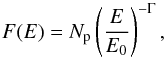 (4)and a log-parabolic one:
 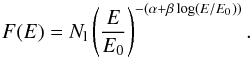 (5)For both models the break energy was set to E0 = 100 MeV and was frozen in the fitting procedure.
The spectral points were calculated by dividing the data set into five logarithmically equal energy bins and a separate likelihood analysis was run for each bin. Unfortunately, PKS 0048−097 is too faint to obtain flux points in the highest energies in the GeV domain. In this case (TS < 9), only the flux upper limits were derived. A one-sigma butterfly contour was calculated using the covariance matrix obtained with the gtlike procedure (Abdo et al. 2009b). The parameters of the spectral fit and the test statistic (TS) for each model and time interval are collected in Table 5. The TS for each interval favours the log-parabolic scenario for the Fermi/LAT data. The log-parabolic fits and the spectral points are shown in the νFν representation in Fig. 7. We recall that in the log-parabolic model the α parameter corresponds to the spectral index, while β gives information about the curvature. The spectral parameters collected in Table 5 do not show significant spectral variability; α is almost constant within the error bars. The curvature parameter changes, but again uncertainties are too large to confirm or exclude significant changes of this parameter. Furthermore, for the B flare β = 0.04 ± 0.04, which means that here a scenario with zero curvature is also possible, which reduces to a single power-law description.
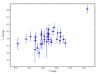 |
Fig. 4 Colour–magnitude plot for PKS 0048−097. Each point corresponds to seven days of binned observations. |
Summary of z-transformed discrete correlation function.
Power-law and log-parabolic fit parameters to Fermi/LAT data.
3.2. Colour–magnitude relation
Figure 4 shows the colour–magnitude diagram for the optical observations of PKS 0048−097 obtained with KAIT and Catalina. Neither a bluer-when-brighter nor a redder-when-brighter chromatism is found in data. The result is consistent with those reported by Ikejiri et al. (2011) and Wierzcholska et al. (2015) for this blazar. The Pearson correlation coefficient calculated for the colour–magnitude relation is 0.45 ± 0.11 (see Appendix A for details on how the uncertainty was estimated). We also note that the optical observations of PKS 0048−097 were not corrected for the contribution of the host galaxy or for the contamination from the emission of the accretion disc.
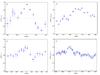 |
Fig. 5 Estimate of the cross-correlation function for different time lags for long-term light curve of PKS 0048−097 (see Fig. 1). All data are binned in weekly averaged intervals. The following subplots show the CCF for a) optical flux in V band, FV versus optical flux in R band, FR as a function of time delay; b) optical flux in V band, FV versus radio flux FRADIO as a function of time delay; c) optical flux in V band, FV versus γ-ray integrated flux Iγ as a function of time delay; d) radio flux, FRADIO versus γ-ray integrated flux, Iγ as a function of time delay. |
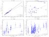 |
Fig. 6 Subplot a) shows the comparison of the optical flux in R (FR) and V (FV) band for PKS 0048−097 for simultaneous observations. The Pearson correlation coefficients for the two cases of a full set of data – solid line and without one data point (in right upper corner in the plot) – dashed line, are provided in the lower right corner. The following subplots show the relation for shifted light curves for b) the radio flux, FRADIO vs. FV; c) integrated gamma-ray flux, Iγ vs. FV; and d) Iγ vs. FRADIO. The light curves are shifted by Δt according to τmax shown in Table 4. In the lower right corner the Pearson correlation coefficients are provided. |
4. Multi-frequency correlations
The simultaneous long-term multi-frequency observations of PKS 0048−097 readily allow for correlation studies. The standard way to quantify possible relations between two datasets is the discrete correlation function (DCF) following Edelson & Krolik (1988). Unfortunately, this method does not work for sparse and non-uniformly sampled light curves. In this case, the cross-correlation function can be better estimated by the z-transformed discrete correlation function (ZDCF). The algorithm has been described in detail by Alexander (1997).
The ZDCF was calculated for four cases: a comparison of optical data in R and V band, optical data in V band and radio data, optical data in V band and γ-ray data, and radio data and γ-ray. To find the peak location for the ZDCF, a maximum-likelihood was calculated for each case using the PLIKE algorithm (Alexander 2013). The peak location, τmax, represents the most probable time-lag between the two light curves. For each combination of the two light curves, we calculated the following quantities: τmax, ZDCF(τmax), and the Pearson correlation coefficient for the given light curves shifted according to the τmax. The results are gathered in Table 4.
In all the cases the flux-flux relation for offset Δt = 0 and for Δt = τmax are presented in Fig. 5. If necessary, the light curves were binned according to the bins of the Fermi/LAT light curves. For the flux-flux relation the Pearson correlation coefficient was calculated, and its error was estimated using a Monte Carlo simulation (see Appendix A for details). Then the flux-flux relation was fitted with a linear function.
The calculated ZDCF values strongly suggest a correlation between the optical observations in V and R band with a time-lag of zero days. For the other comparisons, no significant correlations for any time-lag were found. Radio and optical data show a maximum of the ZDCF function for a time lag of about 200 days with a correlation coefficient of 0.5, which does not allow stating it as significant. For γ-ray and optical data the maximum of ZDCF does not exceed 0.5. Similar results were also found for the radio and γ-ray data set. On the other hand, for the second and fourth case (comparison of optical – radio and γ-ray – radio) the Pearson correlation coefficient calculated for the corresponding τmax (see Table 4) is about 0.6. This indicates a weak correlation between the emission at the two mentioned wavelengths. We note here that Pearson’s correlation coefficient was calculated for binned data in seven-day intervals. This may influence the results because in this case the compared data are only quasi-simultaneous. Moreover, as mentioned before, γ-ray data have large uncertainties, which weakens the statistical importance of this relation.
5. Summary and conclusions
We have presented multi-wavelength monitoring of the blazar PKS 0048−097 for nine years, consisting of observations performed in the radio band with OVRO, in the optical and UV bands with KAIT, Catalina and Swift/UVOT, in the X-ray band with Swift/XRT, and in the high energy γ-ray wavelength with Fermi/LAT. It is the longest published monitoring of this source ever. It is also worth mentioning that except in the optical and radio ranges, PKS 0048−097 was not studied in detail at the different wavelengths. During the period studied here, substantial variability is observed in all wavelengths, which in the case of the optical and radio band is consistent with observations reported for example by Ross (1970), Carswell et al. (1973), Wills et al. (1992), Falomo (1996), Stickel et al. (1993), Sefako et al. (2001). But for the case of other frequencies this is the first time that variability is reported. We observed 3.5 mag variations in the optical band in KAIT data during prominent outbursts, which is the strongest change in the flux for this source ever reported. The variability of PKS 0048−097 that is observed in the other wavelengths seems to be more complex.
The first flare, called A here, is characterized by higher flux in the GeV and optical range. The interpolation of the radio light curve indicates that the observed emission does not show a flare. The second flare discussed in this paper, flare B, is described by higher flux in the GeV, optical, and UV range. However, neither in radio range nor in X-ray are there any significant changes in the flux level. Highly variable emission was quantified using Fvar values, and it indicates that the highest variability is found in the X-ray range and the lowest in the GeV domain.
The correlation studies of PKS 0048−097 show a strong correlation between the optical emission in V and R band and no significant correlations between other wavelengths. The analysis of the cross-correlation function did not show any time lag for which a linear relation could be resolved. The variability observed in different time scales is a common feature for this class of objects. But for the case of the eponymous blazar, the fact that variations are not correlated suggests that the standard, most popular leptonic SSC model might not be enough to describe the emission processes in this object.
The comparison of the optical colour and magnitude of PKS 0048−097 does not show either a bluer-when-brighter or a redder-when-brighter relation for the blazar. The lack of such a relation has also been reported by Ikejiri et al. (2011) and Wierzcholska et al. (2015). The bluer-when-brighter trend is a common feature of the BL Lac-type blazars, where the optical emission is mostly dominated by the synchrotron radiation from the jet.
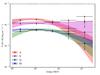 |
Fig. 7 Spectral energy distribution for Fermi/LAT data. Data are fitted using log-parabola models. The following colours corresponds to different time epochs: flare A (red), flare B (magenta), quiescent period (Q) defined in Sect. 3.1 (green), and all data period (M, blue). |
The lack of such behaviour can be caused by the fact that the correlation is hidden by a few overlapping branches, for which chromatism is present individually. For this case it is possible to distinguish separate states in the colour–magnitude diagram, for which bluer-when-brighter relation is evident. This scenario is possible for PKS 0048−097 where the colour–magnitude can disclose substructures with a clear bluer-when-brighter relation.
The optical data we presented were not corrected for either the contribution of the host galaxy or for the contamination from the accretion disc. PKS 0048−097 is a luminous LBL-type blazar (with an optical luminosity of about 1046 erg s-1) with an apparently high accretion rate (Sbarrato et al. 2012). Not taking into account the accretion disc effects may lead to redder-when-brighter results in colour–magnitude diagrams, while the neglecting the host galaxy contribution causes a bluer-when-brighter effect. Hence, according to the optical observations of PKS 0048−097, the lack of any chromatism in the colour-magnitude diagram does not definitely exclude such a relation for the blazar.
The spectral variability studies in GeV energy range show that in this domain the favourable model to describe spectra is the log-parabolic one. Previously, such a model was successfully used in the spectral analysis for other blazars, as reported for instance by Massaro et al. (2004a,b, 2006, 2008), Tramacere et al. (2007, 2009, 2011), Giommi et al. (2005), Perri et al. (2007), Donato et al. (2005).
The studies on the long-term emission in PKS 0048−097 confirm the importance of the simultaneous multi-frequency monitoring of blazars in both the flaring and quiescence states. Our results strongly encourage further monitoring of PKS 0048−097 in the multi-frequency simultaneous campaigns.
Acknowledgments
The author thanks the anonymous referee for constructive comments that greatly improved the manuscript. A.W. acknowledges support by Polish Ministry of Science and Higher Education in Mobility Plus Program. This research has made use of data from the OVRO 40-m monitoring program (Richards et al. 2011), which is supported in part by NASA grants NNX08AW31G and NNX11A043G, and NSF grants AST-0808050 and AST-1109911. The CSS survey is funded by the National Aeronautics and Space Administration under Grant No. NNG05GF22G issued through the Science Mission Directorate Near-Earth Objects Observations Program. The CRTS survey is supported by the US National Science Foundation under grants AST-0909182 and AST-1313422. The author gratefully acknowledges the optical, X-ray, and γ-ray observations provided by the KAIT, Swift and Fermi teams, respectively. This research was supported in part by PLGrid Infrastructure. The plots presented in this paper are rendered using Matplotlib (Hunter 2007).
References
- Abdo, A. A., Ackermann, M., Ajello, M., et al. 2009a, ApJS, 183, 46 [NASA ADS] [CrossRef] [Google Scholar]
- Abdo, A. A., Ackermann, M., Ajello, M., et al. 2009b, ApJ, 707, 1310 [NASA ADS] [CrossRef] [Google Scholar]
- Abdo, A. A., Ackermann, M., Agudo, I., et al. 2010a, ApJ, 716, 30 [NASA ADS] [CrossRef] [Google Scholar]
- Abdo, A. A., Ackermann, M., Ajello, M., et al. 2010b, ApJS, 188, 405 [NASA ADS] [CrossRef] [Google Scholar]
- Abramowski, A., Acero, F., et al. (H.E.S.S. Collaboration) 2013, A&A, 559, A136 [NASA ADS] [CrossRef] [EDP Sciences] [Google Scholar]
- Abramowski, A., Aharonian, F., et al. (H.E.S.S. Collaboration) 2014a, A&A, 564, A9 [NASA ADS] [CrossRef] [EDP Sciences] [Google Scholar]
- Abramowski, A., Aharonian, F., et al. (H.E.S.S. Collaboration) 2014b, A&A, 571, A39 [NASA ADS] [CrossRef] [EDP Sciences] [Google Scholar]
- Aharonian, F., Akhperjanian, A. G., Bazer-Bachi, A. R., et al. 2007, ApJ, 664, L71 [Google Scholar]
- Alexander, T. 1997, in Astronomical Time Series, eds. D. Maoz, A. Sternberg, & E. M. Leibowitz, Astrophys. Space Sci. Lib., 218, 163 [Google Scholar]
- Alexander, T. 2013, ArXiv e-prints [arXiv:1302.1508] [Google Scholar]
- Atwood, W. B., Abdo, A. A., Ackermann, M., et al. 2009, ApJ, 697, 1071 [NASA ADS] [CrossRef] [Google Scholar]
- Band, D. L., & Grindlay, J. E. 1985, ApJ, 298, 128 [NASA ADS] [CrossRef] [Google Scholar]
- Barthelmy, S. D., Barbier, L. M., Cummings, J. R., et al. 2005, Space Sci. Rev., 120, 143 [NASA ADS] [CrossRef] [Google Scholar]
- Begelman, M. C., Blandford, R. D., & Rees, M. J. 1984, Rev. Mod. Phys., 56, 255 [NASA ADS] [CrossRef] [Google Scholar]
- Böttcher, M. 2007, Ap&SS, 309, 95 [NASA ADS] [CrossRef] [Google Scholar]
- Burrows, D. N., Hill, J. E., Nousek, J. A., et al. 2005, Space Sci. Rev., 120, 165 [NASA ADS] [CrossRef] [Google Scholar]
- Carswell, R. F., Strittmatter, P. A., Disney, M. J., Hoskins, D. G., & Murdoch, H. S. 1973, Nature Phys. Sc., 246, 89 [NASA ADS] [CrossRef] [Google Scholar]
- Cohen, D. P., Romani, R. W., Filippenko, A. V., et al. 2014, ApJ, 797, 137 [NASA ADS] [CrossRef] [Google Scholar]
- Dermer, C. D., Schlickeiser, R., & Mastichiadis, A. 1992, A&A, 256, L27 [NASA ADS] [Google Scholar]
- Donato, D., Sambruna, R. M., & Gliozzi, M. 2005, A&A, 433, 1163 [NASA ADS] [CrossRef] [EDP Sciences] [Google Scholar]
- Drake, A. J., Djorgovski, S. G., Mahabal, A., et al. 2009, ApJ, 696, 870 [NASA ADS] [CrossRef] [MathSciNet] [Google Scholar]
- Edelson, R. A., & Krolik, J. H. 1988, ApJ, 333, 646 [NASA ADS] [CrossRef] [Google Scholar]
- Falomo, R. 1996, MNRAS, 283, 241 [NASA ADS] [Google Scholar]
- Fossati, G., Maraschi, L., Celotti, A., Comastri, A., & Ghisellini, G. 1998, MNRAS, 299, 433 [NASA ADS] [CrossRef] [Google Scholar]
- Gehrels, N., Chincarini, G., Giommi, P., et al. 2004, ApJ, 611, 1005 [NASA ADS] [CrossRef] [Google Scholar]
- Giommi, P., Piranomonte, S., Perri, M., & Padovani, P. 2005, A&A, 434, 385 [NASA ADS] [CrossRef] [EDP Sciences] [Google Scholar]
- Giommi, P., Blustin, A. J., Capalbi, M., et al. 2006, A&A, 456, 911 [NASA ADS] [CrossRef] [EDP Sciences] [Google Scholar]
- Giommi, P., Polenta, G., Lähteenmäki, A., et al. 2012, A&A, 541, A160 [NASA ADS] [CrossRef] [EDP Sciences] [Google Scholar]
- Gupta, A. C., Acharya, B. S., Bose, D., Chitnis, V. R., & Fan, J.-H. 2008, Chin. J. Astron. Astrophys, 8, 395 [NASA ADS] [CrossRef] [Google Scholar]
- Hunter, J. D. 2007, Comp. Sci. Eng., 9, 90 [Google Scholar]
- Ikejiri, Y., Uemura, M., Sasada, M., et al. 2011, PASJ, 63, 639 [NASA ADS] [Google Scholar]
- Kalberla, P. M. W., Burton, W. B., Hartmann, D., et al. 2005, A&A, 440, 775 [NASA ADS] [CrossRef] [EDP Sciences] [Google Scholar]
- Konigl, A. 1981, ApJ, 243, 700 [NASA ADS] [CrossRef] [Google Scholar]
- Kotilainen, J. K., Falomo, R., & Scarpa, R. 1998, A&A, 336, 479 [NASA ADS] [Google Scholar]
- Landoni, M., Falomo, R., Treves, A., et al. 2012, A&A, 543, A116 [NASA ADS] [CrossRef] [EDP Sciences] [Google Scholar]
- Li, W., Filippenko, A. V., Chornock, R., & Jha, S. 2003, PASP, 115, 844 [NASA ADS] [CrossRef] [Google Scholar]
- Li, W. D., Filippenko, A. V., Treffers, R. R., et al. 2000, in AIP Conf. Ser., 522, eds. S. S. Holt, & W. W. Zhang, 103 [Google Scholar]
- Mannheim, K., & Biermann, P. L. 1992, A&A, 253, L21 [NASA ADS] [Google Scholar]
- Marscher, A. P., & Gear, W. K. 1985, ApJ, 298, 114 [NASA ADS] [CrossRef] [Google Scholar]
- Massaro, E., Perri, M., Giommi, P., & Nesci, R. 2004a, A&A, 413, 489 [NASA ADS] [CrossRef] [EDP Sciences] [Google Scholar]
- Massaro, E., Perri, M., Giommi, P., Nesci, R., & Verrecchia, F. 2004b, A&A, 422, 103 [NASA ADS] [CrossRef] [EDP Sciences] [Google Scholar]
- Massaro, E., Tramacere, A., Perri, M., Giommi, P., & Tosti, G. 2006, A&A, 448, 861 [NASA ADS] [CrossRef] [EDP Sciences] [Google Scholar]
- Massaro, F., Tramacere, A., Cavaliere, A., Perri, M., & Giommi, P. 2008, A&A, 478, 395 [NASA ADS] [CrossRef] [EDP Sciences] [Google Scholar]
- Mattox, J. R., Bertsch, D. L., Chiang, J., et al. 1996, ApJ, 461, 396 [NASA ADS] [CrossRef] [Google Scholar]
- Mücke, A., Protheroe, R. J., Engel, R., Rachen, J. P., & Stanev, T. 2003, Astropart. Phys., 18, 593 [NASA ADS] [CrossRef] [Google Scholar]
- Nolan, P. L., Abdo, A. A., Ackermann, M., et al. 2012, ApJS, 199, 31 [NASA ADS] [CrossRef] [Google Scholar]
- Padovani, P., & Giommi, P. 1995, ApJ, 444, 567 [NASA ADS] [CrossRef] [Google Scholar]
- Perri, M., Maselli, A., Giommi, P., et al. 2007, A&A, 462, 889 [NASA ADS] [CrossRef] [EDP Sciences] [Google Scholar]
- Pica, A. J., Smith, A. G., Webb, J. R., et al. 1988, AJ, 96, 1215 [NASA ADS] [CrossRef] [Google Scholar]
- Plotkin, R. M., Anderson, S. F., Hall, P. B., et al. 2008, AJ, 135, 2453 [NASA ADS] [CrossRef] [Google Scholar]
- Poole, T. S., Breeveld, A. A., Page, M. J., et al. 2008, MNRAS, 383, 627 [NASA ADS] [CrossRef] [Google Scholar]
- Poutanen, J., Zdziarski, A. A., & Ibragimov, A. 2008, MNRAS, 389, 1427 [NASA ADS] [CrossRef] [Google Scholar]
- Richards, J. L., Max-Moerbeck, W., Pavlidou, V., et al. 2011, ApJS, 194, 29 [NASA ADS] [CrossRef] [Google Scholar]
- Richmond, M., Treffers, R. R., & Filippenko, A. V. 1993, PASP, 105, 1164 [NASA ADS] [CrossRef] [Google Scholar]
- Roming, P. W. A., Kennedy, T. E., Mason, K. O., et al. 2005, Space Sci. Rev., 120, 95 [NASA ADS] [CrossRef] [Google Scholar]
- Ross, H. N. 1970, Nature, 226, 431 [NASA ADS] [CrossRef] [Google Scholar]
- Saito, S., Stawarz, Ł., Tanaka, Y. T., et al. 2013, ApJ, 766, L11 [NASA ADS] [CrossRef] [Google Scholar]
- Sbarrato, T., Ghisellini, G., Maraschi, L., & Colpi, M. 2012, MNRAS, 421, 1764 [NASA ADS] [CrossRef] [Google Scholar]
- Schlafly, E. F., & Finkbeiner, D. P. 2011, ApJ, 737, 103 [NASA ADS] [CrossRef] [Google Scholar]
- Schlegel, D. J., Finkbeiner, D. P., & Davis, M. 1998, ApJ, 500, 525 [NASA ADS] [CrossRef] [Google Scholar]
- Sefako, R. R., de Jager, O. C., & Winkler, H. 2001, in AIP Conf. Ser., 558, eds. F. A. Aharonian, & H. J. Völk, 732 [Google Scholar]
- Sikora, M., Begelman, M. C., & Rees, M. J. 1994, ApJ, 421, 153 [NASA ADS] [CrossRef] [Google Scholar]
- Stickel, M., Fried, J. W., & Kuehr, H. 1993, A&AS, 98, 393 [NASA ADS] [Google Scholar]
- Tramacere, A., Giommi, P., Massaro, E., et al. 2007, A&A, 467, 501 [NASA ADS] [CrossRef] [EDP Sciences] [Google Scholar]
- Tramacere, A., Giommi, P., Perri, M., Verrecchia, F., & Tosti, G. 2009, A&A, 501, 879 [NASA ADS] [CrossRef] [EDP Sciences] [Google Scholar]
- Tramacere, A., Massaro, E., & Taylor, A. M. 2011, ApJ, 739, 66 [NASA ADS] [CrossRef] [Google Scholar]
- Treffers, R. R., Filippenko, A. V., van Dyk, S. D., Paik, Y., & Richmond, M. W. 1995, in Robotic Telescopes. Current Capabilities, Present Developments, and Future Prospects for Automated Astronomy, eds. G. W. Henry & J. A. Eaton, ASP Conf. Ser., 79, 86 [Google Scholar]
- Urry, C. M., & Padovani, P. 1995, PASP, 107, 803 [NASA ADS] [CrossRef] [Google Scholar]
- Usher, P. D., Kolpanen, D. R., & Pollock, J. T. 1974, Nature, 252, 365 [NASA ADS] [CrossRef] [Google Scholar]
- Vaughan, S., Edelson, R., Warwick, R. S., & Uttley, P. 2003, MNRAS, 345, 1271 [NASA ADS] [CrossRef] [Google Scholar]
- Vercellone, S., Striani, E., Vittorini, V., et al. 2011, ApJ, 736, L38 [NASA ADS] [CrossRef] [Google Scholar]
- Wagner, S. 2009, in Astrophysics with All-Sky X-Ray Observations, eds. N. Kawai, T. Mihara, M. Kohama, & M. Suzuki, 186 [Google Scholar]
- Wagner, S. J., & Witzel, A. 1995, ARA&A, 33, 163 [NASA ADS] [CrossRef] [Google Scholar]
- Wierzcholska, A., Ostrowski, M., Stawarz, Ł., Wagner, S., & Hauser, M. 2015, A&A, 573, A69 [NASA ADS] [CrossRef] [EDP Sciences] [Google Scholar]
- Wills, B. J., Wills, D., Breger, M., Antonucci, R. R. J., & Barvainis, R. 1992, ApJ, 398, 454 [NASA ADS] [CrossRef] [Google Scholar]
Appendix A: Error estimation for the Pearson correlation coefficient
To estimate the uncertainty of the Pearson correlation coefficient, one can use the Monte Carlo approach. Here we assumed that a set of points A = { (xi,yi) } is given and each of the point has its own corresponding uncertainty values (Δxi,Δyi). In the first step, for each point new coordinates were drawn randomly according to the normal distribution for which the mean was set to xi (or yi) and the standard deviation to Δxi (or Δyi). This results in a new set of points A′, and its Pearson correlations coefficient is C′.
Repeating the procedure N times gives a set of Pearson coefficients  . If N is large enough, a histogram of the
  should have roughly a Gaussian shape. However, because the Pearson coefficient only has values in the range [− 1,1] it is good to apply a Fisher transformation (see below) on each of the C′ value before making the histogram. An example of such a histogram is shown in Fig. A.1.
To find the uncertainty of the Pearson coefficient, a Gaussian function was fitted to the histogram. The standard deviation of this fit can be used as an estimate of the Pearson coefficient uncertainty of the original set of points A. The value found by fitting should be transformed back by the reverse Fisher transformation.
Fisher transformation
The Fisher transformation allows representing values that span from [− 1,1] in a range of (− ∞,∞). It is defined as follows:  (A.1)and the reverse:
  (A.2)
(A.2)
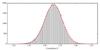 |
Fig. A.1 Histogram of the Monte Carlo-generated set of 105 Pearson correlation coefficients { C′ }. The red line shows the Gaussian fit. The C′ values were transformed with the Fisher transformation. The reverse Fisher transformation of the fit gives a Pearson correlation coefficient equal to 0.87, and its error is estimated to 0.03. |
All Tables
Magnitudes for different epochs from Swift/UVOT data for V, B, U, UVW1, UVM2, and UVW2 filters.
All Figures
|
Fig. 1 Multi-wavelength light curve of PKS 0048−097. Panels from the top to the bottom show the radio observations from the OVRO telescope at 15 GHz; optical (KAIT and Catalina) monitoring in R and V band, Swift/UVOT data in V, B, U, UVW1, UVM2, and UVW2 filters, X-ray observations with Swift/XRT, and Fermi/LAT flux (E> 100 MeV). The horizontal dashed lines in all the panels represent the average flux for all observations presented here. In all the cases (excluding Fermi/LAT data) each point corresponds to one night of observations; for the case of Fermi/LAT monitoring data are binned in week-long intervals. In the Fermi/LAT light curve, flux upper limits are represented with grey points. The time periods corresponding to A and B flares are marked in grey, while the quiescence period Q is plotted in blue. |
| In the text | |
|
Fig. 2 Temporal and spectral variability of PKS 0048−097 observed with Swift/XRT and Fermi/LAT. The following panels present the X-ray temporal and spectral variability and the γ-ray temporal and spectral variability. For Swift/XRT observations one point correspond to one day of observations, while in the case of Fermi/LAT data one point is for weekly integrated observations. We plot the flux upper limits in the Fermi/LAT light curve with grey points. The time periods corresponding to A and B flares are marked in grey, while the quiescence period Q is shown in blue. |
| In the text | |
|
Fig. 3 Fractional variability vs. frequency for each observation regime. The numerical values can be found in Table 3. The colours for the data points are the same as in Fig. 1. |
| In the text | |
|
Fig. 4 Colour–magnitude plot for PKS 0048−097. Each point corresponds to seven days of binned observations. |
| In the text | |
|
Fig. 5 Estimate of the cross-correlation function for different time lags for long-term light curve of PKS 0048−097 (see Fig. 1). All data are binned in weekly averaged intervals. The following subplots show the CCF for a) optical flux in V band, FV versus optical flux in R band, FR as a function of time delay; b) optical flux in V band, FV versus radio flux FRADIO as a function of time delay; c) optical flux in V band, FV versus γ-ray integrated flux Iγ as a function of time delay; d) radio flux, FRADIO versus γ-ray integrated flux, Iγ as a function of time delay. |
| In the text | |
|
Fig. 6 Subplot a) shows the comparison of the optical flux in R (FR) and V (FV) band for PKS 0048−097 for simultaneous observations. The Pearson correlation coefficients for the two cases of a full set of data – solid line and without one data point (in right upper corner in the plot) – dashed line, are provided in the lower right corner. The following subplots show the relation for shifted light curves for b) the radio flux, FRADIO vs. FV; c) integrated gamma-ray flux, Iγ vs. FV; and d) Iγ vs. FRADIO. The light curves are shifted by Δt according to τmax shown in Table 4. In the lower right corner the Pearson correlation coefficients are provided. |
| In the text | |
|
Fig. 7 Spectral energy distribution for Fermi/LAT data. Data are fitted using log-parabola models. The following colours corresponds to different time epochs: flare A (red), flare B (magenta), quiescent period (Q) defined in Sect. 3.1 (green), and all data period (M, blue). |
| In the text | |
|
Fig. A.1 Histogram of the Monte Carlo-generated set of 105 Pearson correlation coefficients { C′ }. The red line shows the Gaussian fit. The C′ values were transformed with the Fisher transformation. The reverse Fisher transformation of the fit gives a Pearson correlation coefficient equal to 0.87, and its error is estimated to 0.03. |
| In the text | |
Current usage metrics show cumulative count of Article Views (full-text article views including HTML views, PDF and ePub downloads, according to the available data) and Abstracts Views on Vision4Press platform.
Data correspond to usage on the plateform after 2015. The current usage metrics is available 48-96 hours after online publication and is updated daily on week days.
Initial download of the metrics may take a while.