| Issue |
A&A
Volume 580, August 2015
|
|
|---|---|---|
| Article Number | A2 | |
| Number of page(s) | 7 | |
| Section | The Sun | |
| DOI | https://doi.org/10.1051/0004-6361/201424431 | |
| Published online | 20 July 2015 | |
Flux rope proxies during 2013 detected by the Solar Dynamics Observatory⋆
Key Laboratory of Solar Activity, National Astronomical Observatories, Chinese Academy of Sciences, 100012 Beijing, PR China
e-mail: This email address is being protected from spambots. You need JavaScript enabled to view it.
Received: 19 June 2014
Accepted: 26 May 2015
Abstract
Context. The relationship between flux ropes and coronal mass ejections (CMEs) is of great importance for understanding the CME initiation, but we do not know how many flux ropes in the atmosphere can be detected.
Aims. We aim to determine the number of flux rope proxies and understand the distribution of the proxies over the visible solar disk.
Methods. By employing the observations from the Atmospheric Imaging Assembly onboard the Solar Dynamics Observatory, we counted the number of the flux rope proxies from 2013 January to 2013 December.
Results. We detected 1354 (3.7 every day) rope proxies during this period and classified them into three types according to their temperature properties and particular (sigmoid) structures. The first type is that the rope proxies are detected in both lower and higher temperature lines. The second is that the rope proxies can only be detected in higher temperature lines, and the third is that the proxies display sigmoid structures in extreme ultraviolet channels. Six hundred and fifty-eight proxies of the 1354 that belong to the first type are tracked by active or eruptive material of filaments or prominences. Four hundred and eighty-seven proxies appear to be rising from the lower atmosphere or brightening in the corona, and belong to the second type. The remaining 209 display sigmoid structures, and they are attributed to the third type. We detected 497 rope proxies, which is 37% of the total, in the northern hemisphere.
Conclusions. Our findings imply a significantly asymmetric distribution of the rope proxies over the visible solar disk.
Key words: Sun: activity / Sun: filaments, prominences / Sun: magnetic fields
Movies are only available in electronic form at http://www.aanda.org
© ESO, 2015
1. Introduction
The flux rope is believed to be an important ingredient for a coronal mass ejection (CME), and one of the physical mechanisms triggering the CME is thought to be the kink instability or the torus instability of the rope (Török & Kliem 2003, 2005; Fan 2005; Kliem & Török 2006; Olmedo & Zhang 2010). Thus, it is important to study flux ropes in detail to obtain a clear understanding of CMEs, which can help us to improve the ability of forecasting CMEs and associated space weather (Li & Zhang 2013a).
There are two principal classes of models for the magnetic configuration of filament-channel fields before eruption: twisted flux ropes and sheared arcades (see review by Mackay et al. 2010). For these initial configurations, the eruption onset has been attributed to either a loss of equilibrium instability (e.g., Forbes & Isenberg 1991; Rachmeler et al. 2009) or magnetic reconnection (e.g., Sturrock 1989; Amari et al. 2000; Titov et al. 2008). The ideal models require the presence of a twisted flux rope before eruption, whereas the reconnection models can operate with either a twisted flux rope or a sheared arcade (Forbes et al. 2006). However, the formation of a flux rope before eruption is not universally accepted. Moore et al. (2001) suggested that the magnetic explosion was unleashed by runaway tether-cutting via implosive/explosive reconnection in the middle of the sigmoid, as in the standard model. In contrast, Karpen et al. (2012) showed that CME onset is due to the start of fast reconnection at the breakout current sheet. Once this reconnection begins, eruption is inevitable. The breakout model invokes reconnection to disrupt the force balance that maintains the highly sheared filament-channel field in the corona (Antiochos et al. 1994; Antiochos 1998; Lynch et al. 2004, 2008; DeVore & Antiochos 2005, 2008; DeVore et al. 2005; Roussev et al. 2007; van der Holst et al. 2007; Zuccarello et al. 2008; Jacobs et al. 2009). In some conditions, the mechanism of flux rope formation by reconnection during flux cancellation (van Ballegooijen & Martens 1989) may operate in a rather similar manner when new flux emerges (Manchester et al. 2004).
The formation and dynamic behavior of flux ropes have been successfully simulated by many authors. Flux ropes emerge from below the photosphere (Archontis & Hood 2012; MacTaggart & Hood 2009; see the review by Hood et al. 2012), although it is not yet clear whether they can emerge as a whole (Manchester et al. 2004; Gibson et al. 2004; Fan 2009; An & Magara 2013; Leake et al. 2013). In addition, the process that a twisted flux rope is formed after a reconnection is also well displayed (Amari et al. 2003; Aulanier et al. 2010). The helical kink instability of a twisted magnetic flux rope can be the initial driver of solar eruptions (Török & Kliem 2005). Continued emergence of a twisted flux rope resulted in the repeated formations and partial eruptions (Chatterjee & Fan 2013), and then developed homologous CMEs (Zhang & Wang 2002).
By extrapolating observed photospheric vector magnetic fields into the corona and assuming linear force-free fields (LFFF; Aulanier & Démoulin 1998), the helical flux ropes overlying the polarity inversion lines were produced and filaments were supported by the dips in the helical field lines (van Ballegooijen & Martens 1989; Priest et al. 1989; Rust & Kumar 1994; Aulanier et al. 1998, 2000; Chae et al. 2001; Aulanier & Démoulin 2003; Gibson & Fan 2006; Dudik et al. 2008). An alternative method for constructing NLFFF models of filaments was developed by van Ballegooijen (2004). In this method, a flux rope was inserted into a potential field based on an observed photospheric magnetogram, and then the field was evolved to an equilibrium state using magneto-frictional relaxation.
Direct observations of flux ropes have been reported by using data from the Yohkoh Soft X-ray Telescope (Tsuneta et al. 1991) and the Atmospheric Imaging Assembly (AIA; Lemen et al. 2012) onboard the Solar Dynamics Observatory (SDO; Pesnell et al. 2012). Although filaments are always considered to be associated with flux ropes, very few cases of observed filaments are sufficiently clear signs of a flux rope, an obvious example was presented by Chae (2000) that the filament appeared as mixtures of bright and dark threads. Early X-ray observations show that there are many sigmoid (S-shaped) structures in the corona, and they are suggested to be twisted magnetic flux ropes (Rust & Kumar 1996). During the eruption of a flux rope, a major flare is always observed (Liu et al. 2003; Patsourakos et al. 2013). Recently, flux ropes are usually detected in AIA higher temperature channels, for example, 131 Å (Zhang et al. 2012). Moreover, flux ropes sometimes appear one by one from the same region with a similar morphology, termed homologous flux ropes (Li & Zhang 2013b). The fine-scale structures of flux ropes can be tracked by erupting material once in a while and are observed in both lower and higher temperature lines (Li & Zhang 2013a; Yang et al. 2014).
Taking advantage of new data and new methods, the structures and evolutions of flux ropes have been explored. Guo et al. (2010) proposed that the magnetic field structure in one section of the filament is a flux rope, while the other is a sheared arcade. Another case showed that a twisted flux rope rose from its source active region, rapidly moving outward (Li & Zhang 2013b). Through continuous tracking, Howard & DeForest (2012) presented the direct observations of a particular flux rope in situ with the same flux rope before ejection from the corona. Furthermore, at least 40% of the observed CMEs have clear flux rope structures (Vourlidas et al. 2013).
The origin of flux ropes in the solar atmosphere has been extensively investigated. It has been reported that a helical flux rope emerged from below the photosphere into the corona along a polarity inversion line (Okamoto et al. 2008). A related possible original mechanism is that the flux rope is built up and heated by the magnetic reconnection in the quasi-separatrix layers (Guo et al. 2013). Green & Kliem (2009) reported that a sigmoid flux rope was formed in the gradual decay phase of an active region and they argued that the inferred flux rope did experience a partial eruption. Savcheva et al. (2012) have explored the scenario of photospheric flux cancellation in more detail, which is the primary formation mechanism of sigmoidal flux ropes in decaying active regions. The flux ropes can exist in the corona before eruptive activities (Tripathi et al. 2009), and play a key role in CME initiation.
Although much evidence has proved the existence of flux ropes in the solar atmosphere, one question remains: how many flux ropes can be detected in the atmosphere? We intend to answer this with current observational data. We count the number of the flux rope proxies from 2013 January to 2013 December, with the observations from the AIA and the Helioseismic and Magnetic Imager (HMI; Scherrer et al. 2012; Schou et al. 2012) onboard the SDO. When we observe a set of extreme ultraviolet (EUV) loops that collectively wind around a central, axial line (Gibson et al. 2004), we consider them as a flux rope proxy. The paper is organized as follows. In Sect. 2 we describe the observational data. The distribution of the ropes over the solar disk and the typical cases are presented in Sect. 3. In Sect. 4, we conclude this study and discuss the results.
2. Observations and data analysis
SDO/AIA observes the full-disk of the Sun in ten wavelength channels with a spatial sampling of 0.̋6 pixel-1 and a cadence of 12 s. The temperature coverage is from ~5000 K to ~20 MK, corresponding to the solar atmosphere from the photosphere to the corona. SDO/HMI provides the measurements of the photospheric Doppler velocity, the line of sight (LOS), and vector magnetic fields. The LOS magnetograms cover the visible solar disk with a pixel size of 0.̋5 and a cadence of 45 s.
The data adopted here were obtained during a whole year (from 2013 January 1 to 2013 December 31). As some flux ropes are more sensitive in higher temperature lines, for example, 131 Å (Zhang et al. 2012), and some in both lower and higher temperature lines, such as 304 Å and 131 Å (Li & Zhang 2013a), we daily checked the 304 Å and 131 Å data.
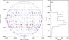 |
Fig. 1 Solar disk distribution (left panel) and latitudinal distribution (right panel) of all the 1354 flux rope proxies. Each blue dot represents a flux rope proxy tracked by a filament eruption (activity). Each red dot represents a rope proxy that appears to be rising from the lower atmosphere or an EUV brightening in the corona, and each green triangle represents a proxy indicated by sigmoid structures. |
3. Results
We counted 1354 flux rope proxies from 2013 January to 2013 December by checking the daily observations of AIA 304 Å and 131 Å. These proxies can be roughly classified into three types. The first type are the proxies that are tracked by active or eruptive material of filaments and can be detected in both lower and higher temperature lines. The second are the proxies that appear to be rising from the lower atmosphere or brightening in the corona and can only be detected in higher temperature lines, and the third type are the proxies that display sigmoid structures in EUV channels. Figure 1 shows solar disk distribution (left panel) and latitudinal distribution (right panel) of the rope proxies. Each blue dot represents a flux rope proxy tracked by a filament eruption (activity). Each red dot represents a rope proxy that appears to be rising from the low atmosphere or an EUV brightening in the higher temperature line, and each green triangle marks a proxy indicated by sigmoid structures. In Fig. 1a, many rope proxies are located at the eastern and western limbs of the Sun. There are two reasons for this phenomenon. First, all the rope proxies rising beyond the solar disk are projected at the limbs. Secondly, although some rope proxies are rooted in the far side of the Sun, they are also projected on the limbs when they are detected in the higher atmosphere. Six hundred fifty-eight rope proxies of the 1354 are tracked by active or eruptive material of filaments or prominences. Four hundred eighty-seven proxies appear as twist structures in higher temperature channels rising from the lower atmosphere or brightening in the corona. The remaining 209 display sigmoid structures in higher temperature channels. During 2013, there were some particularly active regions. In each of these active regions, many rope proxies were detected, so the data points in Fig. 1a appear to show some clustering. Four hundred ninety-seven rope proxies, which is 37% of the total rope proxies, are detected in the northern hemisphere, the other 857 rope proxies in the southern hemisphere. The latitudinal distribution (Fig. 1b) shows that the peak distribution (218 proxies) in the northern hemisphere is at 15°, in the southern hemisphere the peak (270 proxies) is located at 23°. Moreover, there are 34 rope proxies at high latitude (>S60°) in the southern hemisphere, which is much more (3 rope proxies) than in the northern hemisphere. These observations imply a significantly asymmetric distribution of the rope proxies both in the active-region belt and in the higher latitudes over the visible solar disk.
3.1. First type of flux rope proxies: tracked by active or eruptive material of filaments/prominences
An example of the first type of flux rope proxies is shown in Fig. 2. This is a filament-associated flux rope proxy located at the neutral line of active region AR 11938 on 2013 December 31 (see movie 1). Before the detectable rope proxy, the filament (Fig. 2a) first brightened at 05:03 UT. Almost 20 min later (Fig. 2b), the main body of the filament brightened, and the brightening material moved bi-directional along the neutral line. At 05:30 UT (Fig. 2c), the outline of the rope striding over the active region was tracked by the brightening filament material. About 3 min later, the endpoints of the rope proxy, which were rooted in the faculae of the active region (windows A and B in Figs. 2c and g, see also Figs. 2h1 and h2) were evident. The rope proxy did not erupt, instead, it darkened gradually. At 09:42 UT, it could not be detected wholly. The rope proxy was not only detected in the higher temperature lines (e.g., 131 Å, Figs. 2a−d), but also in the lower temperature lines (304 Å and 171 Å). For comparison with the 131 Å image in Fig. 2d, we display in Figs. 2e and f the corresponding 304 Å and 171 Å observations. We note that the upper part of the rope, which appeared as twisted structures, was similar in the different lines. Since the northern part of the structure (in area A in Fig. 2) is so similar in the three AIA bands, it most likely only consists of relatively cool plasma, with the 131 Å emission being due to the Fe VIII lines in this channel (see O’Dwyer et al. 2010). The structure located between areas A and B shows differences between the hotter 131 Å band and the cooler 171 and 304 Å bands, for instance, the part marked by the arrows in Fig. 2d is only visible in the 131 Å band, indicating that this part must be hot.
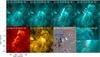 |
Fig. 2 Panels a)–d): sequence of AIA 131 Å images showing a flux rope proxy tracked by active material of a filament on 2013 December 31. Panels e)–g): corresponding AIA 304 Å and 171 Å images and HMI magnetorgram when the flux rope was well observed. Panels h1), h2): two expanded 131 Å images outlined by rectangles A and B in panel c). The arrows in panel d) mark the parts of the structure that are only visible in the 131 Å band, and the blue and red curves in panels h1) and h2) are contours of the corresponding positive and negative magnetic fields. An animation (movie1.mp4) of the 304 Å and 131 Å channels shown in this figure is available online. |
Figure 3 shows an event that occurred on 2013 August 22 (see movie 2). A prominence began to rise up at 13:14 UT at the western limb of the Sun, and then the prominence appeared as a kink structure (Fig. 3a). About 40 min later (Figs. 3b−d), the kink structure was well developed in the AIA field of view. In different temperature channels, the kink structure was similar, but flare loops (denoted by the arrow) were seen only in the high-temperature channel (e.g., 131 Å, see Fig. 3d) near the footpoints of the prominence, indicating there was a heating process. Then the prominence erupted as a whole at 14:31 UT, and a slow CME with an average speed of 190 km s-1 and a C2.4 flare were produced.
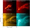 |
Fig. 3 AIA 304 Å (panels a), b)), 171 Å (panel c)), and 131 Å (panel d)) images showing an eruptive prominence on 2013 August 22. The arrow in panel c) denotes the kink of the prominence and the arrow in panel d) a closed brightening loop. An animation (movie2.mp4) of the 304 Å channel shown in this figure is available online. |
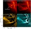 |
Fig. 4 Panels a) and b): AIA 304 Å images showing an eruptive prominence on 2013 October 27. Panels c) and d): differential images between 04:48 UT and 05:21 UT in 171 Å and 131 Å, respectively. The arrow in panel d) denotes a closed brightening loop. An animation (movie3.mp4) of the 304 Å channel shown in this figure is available online. |
Figure 4 shows another prominence event that took place on 2013 Octomber 27 on the eastern limb of the Sun (see also movie 3). Part of the prominence material brightened at 04:44 UT and then the prominence clearly rose up (Fig. 4a). At 05:21 UT, the prominence developed into an arch structure (Figs. 4b−d), with both legs showing indications of twist (e.g., see Fig. 4c). Ten minutes later, the top of the arch broke off, and the majority of the prominence material fell from high altitude to the solar surface. As displayed in Fig. 4, this arch structure was similar in different temperature channels, and flare loops were seen (denoted by an arrow in Fig. 4d) near one footpoint of the arch in the hot band.
3.2. Second type of flux rope proxies: rising from the lower atmosphere detected in hot temperature channels
Different from these examples, in which the rope proxies can be detected in both lower and higher temperature lines, here we present two events for which the rope proxies are detected mainly in the higher temperature lines. The first event took place on 2013 May 22 in AR 11754 (see movie 4). This event was investigated by Li & Zhang (2013b) and Cheng et al. (2014). These authors have performed a detailed analysis of the hot channel, providing strong evidence that the channel has the magnetic structure of a flux rope. This proxy initiated with a partial eruption of a filament (see movie 4 and Figs. 5a and d) at 12:10 UT. The filament material brightened and moved along the two directions of the filament channel during the following 8 min. At 12:20 UT (movie 4), the rope that contained the filament appeared. It rose from the lower atmosphere and also extended along the filament channel (Fig. 5b). Almost 6 min later (at 12:45 UT, Fig. 5c), the rope was well developed. Then the flux rope erupted rapidly, followed by an M5.0 flare (which occurred at 13:08 UT) and a CME (detected near 13:25 UT). This rope was different from that displayed in Figs. 2−4, for instance, the main body of this rope cannot be detected in the lower temperature lines (e.g., 304 Å and 171 Å, see Figs. 5e and f).
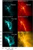 |
Fig. 5 Panels a)−c): AIA 131 Å base-difference images (the base image is taken at 12:00 UT) showing a flux rope rising from lower atmosphere on 2013 May 22. Panel d): AIA 304 Å image showing the filament at the early rising phase of the flux rope. Panels e), f): corresponding AIA 304 Å and 171 Å images at 12:45 UT, respectively. An animation (movie4.mp4) of the 131 Å channel shown in this figure is available online. |
Another event took place on 2013 December 29 in AR 11938 (see movie 5). The rope proxy initiated with a failed eruption of a filament (see Fig. 6a) at 01:12 UT. The filament material brightened and moved along the two directions of the filament channel during the following 15 min. At 01:27 UT, the rope proxy that contained the filament appeared. It rose from the lower atmosphere and also extended along the filament channel. Almost 10 min later (at 01:36 UT, Fig. 6c), the proxy was well developed, and the twist (see the dotted curves) was well indicated. It extended over the active region, with two endpoints rooting in the faculae of the active region. About 1 h later, the rope proxy faded away. This rope proxy was to some extent similar to that displayed in Fig. 2 because both of them extended over active regions and were rooted in the faculae. But the difference was also obvious: the main body of this rope proxy cannot be detected in the lower temperature lines, for instance, 304 and 171 Å (see Figs. 6e and f).
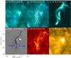 |
Fig. 6 AIA 131 Å images (panels a) and b)) and the differential image between 01:12 UT and 01:36 UT (panel c)) showing a flux rope proxy rising from lower atmosphere on 2013 December 29. Panels d)−f): corresponding HMI magnetogram, AIA 304 Å, and 171 Å images. The blue and red solid curves in panel b) are the contours of the positive and negative underlying magnetic fields. The red dotted curves in panel c) outline the twisted threads of the flux rope proxy, and the black curve in panel d) outlines the general shape of the filament. An animation (movie5.mp4) of the 131 Å channel shown in this figure is available online. |
3.3. Third type of flux rope proxies: appearing as sigmoid structures in hot channels
The first event of a sigmoid rope proxy appeared in hot temperature channels (see Figs. 7a−c) in AR 11890 (Fig. 7f) on 2013 November 11 (see movie 6). A sigmoid structure (S1) of the rope proxy that connected strong negative fields with weak positive magnetic fields (see the red curves in Figs. 7b, c and f) was first observed at 13:12 UT and was more clearly at 13:21 UT (Fig. 7b). About 3 min later, another sigmoid structure (S2) of the rope proxy appeared with one endpoint rooted in the same strong negative fields, but the other one was place in the strong positive fields (see the blue curves in Figs. 7c and f). These two strong opposite-polarity fields consisted of the main body of the active region. S2 gradually developed and slowly rose up, and at 13:42 UT, S2 fully concealed S1, and then the rope proxy darkened and fainted away near 14:21 UT. A slow CME with an average speed of 250 km s-1 and a C4.8 flare with a peak time at 13:37 UT were produced. Figures 7d and e display the 304 Å and 171 Å images at 13:33 UT. Compared with Fig. 7c, the rope proxy cannot be observed in the lower temperature channels.
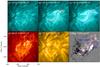 |
Fig. 7 Panels a)−c): AIA 131 Å images showing a sigmoid flux rope proxy on 2013 November 11. The red curve S1 in panel b) denotes a sigmoid structure. The blue curve S2 in panel c) outlines another sigmoid structure, and the red dotted curve S1 duplicates curve S1 in panel b). Panels d)−f): corresponding AIA 304 Å and 171 Å images and HMI magnetogram. The red and blue curves in panel f) delineate the duplicates of curves S1 and S2 in panel c). An animation (movie6.mp4) of the 131 Å channel shown in this figure is available online. |
The second example (see Figs. 8a−c) occurred in AR 11817 on 2013 August 14 (see also movie 7). The fine structure of the rope proxy that connected strong positive-negative magnetic fields (see the yellow curves in Figs. 8a and 8f) were first observed near 10:22 UT, and then other fine structures, which displayed an increasingly sigmoidal shape, successively appeared (e.g., see Figs. 8b, c and f). The three S-shaped structures outlined by the dotted lines in Figs. 8a–c appeared to be different structures that were sequentially illuminated, with their footpoints rooted in two strong opposite-polarity fields (Fig. 8f), which consisted of the main body of the active region. A twisted structure, that is, a flux rope proxy, is indicated by the crossing lines in panel f. At 11:28 UT, the rope proxy was well developed, then it darkened and fainted away near 12:16 UT. Figures 8d and e display the 304 Å and 171 Å images at 11:25 UT. Compared with Fig. 8c, we note that the S-shaped structures are not detected in the lower temperature lines, but a confined C1.5 flare with a peak time at 10:37 UT was produced.
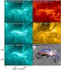 |
Fig. 8 Panels a)−c): AIA 131 Å images showing a sigmoid flux rope proxy on 2013 August 14. The yellow, red and blue dotted curves in panels a)−c) delineate the fine structures of the rope proxy. Panels d)−f): corresponding AIA 304 Å and 171 Å images and HMI magnetogram. The three colored curves in panel f) are the same as the dotted curves in panels a)–c). An animation (movie7.mp4) of the 131 Å channel shown in this figure is available online. |
4. Conclusions and discussion
We counted for the first time the number of the flux rope proxies from 2013 January to 2013 December by daily examining the AIA 304 Å and 131 Å observations, and we detected 1354 rope proxies (3.7 rope proxies per day) during this period. There are three types of rope proxies. For the first type, the rope proxies are detected in both lower and higher temperature wavelengths. For the second type, the rope proxies can only be detected in higher temperature lines, and for the third type the proxies display sigmoid structures in EUV channels. Six hundred fifty-eight proxies of the 1354 that belong to the first type are tracked by active or eruptive material of filaments or prominences. Four hundred eighty-seven proxies appear to be twisted structures in hot channels rising from the lower atmosphere or brightening in the corona, and the remaining 209 display sigmoid structures in hot channels. We detected 37% (497 rope proxies) of the 1354 proxies in the northern hemisphere, implying a significantly asymmetric distribution of the ropes over the full disk of the Sun.
Several previous case studies have shown that flux ropes are detected in X-ray and in higher temperature EUV wavelengths (Rust & Kumar 1996; Zhang et al. 2012; Li & Zhang 2013), or at both lower and higher temperature wavelengths, for example, 304 Å and 131 Å (Li & Zhang 2013a). Based on the statistical analysis of these 1354 rope proxies, we note that all the rope proxies can be detected in higher temperature channels. This means that in the low-beta flux rope models for filaments or prominences and filament channels, the presence of cool material is generally considered to be of only secondary influence on the magnetic structure (Mackay et al. 2010). DeVore & Antiochos (2000) have displayed a mixture of sigmoidal arcade-like field lines and helical (flux-rope) field lines in their prominence model, and their study is consistent with the assumption we made here.
We only observed the second and third types of flux rope proxies at high temperature. The second type of flux rope proxies shows that the high-temperature loops are twisted (e.g., see Figs. 5c and 6c). However, the sigmoidal loops of the third type of flux rope proxies have sheared structures (see Figs. 7c and 8c). This geometrical difference between the two types may exist for real in the solar atmosphere, but we cannot rule out the possibility that the difference results from differences in the viewing angle.
Early observations and simulations have recognized that the ropes in the solar atmosphere either emerge from below the photosphere (Okamoto et al. 2008; Leake et al. 2013), or are produced by reconnection in the atmosphere (Amari et al. 2003; Savcheva et al. 2012). Here we cannot determine whether some rope proxies emerge from below the photosphere or not, but surely some rope proxies rise from the lower atmosphere, for example, the rope on 2013 May 22 (see Figs. 5a and b). To confirm the rope emerging from below the photosphere, we need to analyze the detailed evolution of magnetic fields. To do this, vector magnetic field observations with higher resolution are needed.
The asymmetric distribution of the rope proxies over the whole Sun is a new finding. From checking the sunspot number in the southern and the northern hemispheres, we find that the number in the two hemispheres is almost equal, indicating that the asymmetry may not be associated with the sunspot number. The excess of flux rope proxies in the southern hemisphere may be caused by two reasons. The first reason is that more active regions in the southern hemisphere contain rope proxies, or some active regions have multiple rope proxies (Lites 2005). The second reason is that more eruptive (or active) filaments that track the rope proxies are detected in the southern hemisphere. In Fig. 1a, more filament-associated rope proxies are plotted in the higher latitudes of the southern hemisphere. These observations may also imply a north-south asymmetry of filaments; Li et al. (2010) reported that the asymmetry of filaments in solar cycles 16−21 is a common phenomenon. In solar cycles 16−20, there are more filaments in the northern than in the southern hemisphere. However, in cycle 21, the southern hemisphere is dominant. Joshi et al. (2009) presented the results of a study of the spatial distribution and asymmetry of solar active prominences (SAP) for the period 1996 through 2007 (solar cycle 23). During the rising phase of the cycle, the number of SAP events are roughly equal in the northern and southern hemispheres, but the activity in the southern hemisphere was dominant since 1999. Using sunspot groups and sunspot areas from May 1996 to February 2007, Li et al. (2009) found that solar activity for cycle 23 is also dominant in the southern hemisphere. They forecast that the solar activities in cycle 24 will remain dominant in the southern hemisphere. These observations and forecast agree with the result in this work.
We should mention that we have only detected the lower limit number of flux rope proxies in the solar atmosphere over one year, and some small and/or unclear rope proxies may be excluded. In addition, some important questions that we did not consider here are how many ropes erupted over one year, and how many erupted ropes are associated with CMEs? The next work is to examine rope evolutions and to determine the number of erupted ropes and the relationship between the erupted ropes and CMEs.
Online material
Movie of Fig. 2 Access Supplementary Material
Movie of Fig. 3 Access Supplementary Material
Movie of Fig. 4 Access Supplementary Material
Movie of Fig. 5 Access Supplementary Material
Movie of Fig. 6 Access Supplementary Material
Movie of Fig. 7 Access Supplementary Material
Movie of Fig. 8 Access Supplementary Material
Acknowledgments
We are grateful to the anonymous referee for the constructive comments and helpful suggestions to improve the manuscript. This work is supported by the National Natural Science Foundations of China 11025315, the National Basic Research Program of China under grant 2011CB811403, the National Natural Science Foundations of China (11221063, 11203037 and 11303050), the CAS Project KJCX2-EW-T07 and the Strategic Priority Research Program-The Emergence of Cosmological Structures of the Chinese Academy of Sciences, Grant No. XDB09000000. The data are used courtesy of NASA/SDO and the AIA and HMI science teams.
References
- Amari, T., Luciani, J. F., Mikic, Z., & Linker, J. 2000, ApJ, 529, L49 [NASA ADS] [CrossRef] [PubMed] [Google Scholar]
- Amari, T., Luciani, J. F., Aly, J. J., Mikic, Z., & Linker, J. 2003, ApJ, 585, 1073 [NASA ADS] [CrossRef] [Google Scholar]
- An, J. M., & Magara, T. 2013, ApJ, 773, 21 [NASA ADS] [CrossRef] [Google Scholar]
- Antiochos, S. K. 1998, ApJ, 502, L181 [NASA ADS] [CrossRef] [Google Scholar]
- Antiochos, S. K., Dahlburg, R. B., & Klimchuk, J. A. 1994, ApJ, 420, L41 [Google Scholar]
- Archontis, V., & Hood, A. W. 2012, A&A, 537, A62 [NASA ADS] [CrossRef] [EDP Sciences] [Google Scholar]
- Aulanier, G., & Demoulin, P. 1998, A&A, 329, 1125 [NASA ADS] [Google Scholar]
- Aulanier, G., & Démoulin, P. 2003, A&A, 402, 769 [NASA ADS] [CrossRef] [EDP Sciences] [Google Scholar]
- Aulanier, G., Demoulin, P., van Driel-Gesztelyi, L., Mein, P., & Deforest, C. 1998, A&A, 335, 309 [NASA ADS] [Google Scholar]
- Aulanier, G., Srivastava, N., & Martin, S. F. 2000, ApJ, 543, 447 [NASA ADS] [CrossRef] [Google Scholar]
- Aulanier, G., Török, T., Démoulin, P., & DeLuca, E. E. 2010, ApJ, 708, 314 [Google Scholar]
- Chae, J. 2000, ApJ, 540, L115 [NASA ADS] [CrossRef] [Google Scholar]
- Chae, J., Wang, H., Qiu, J., et al. 2001, ApJ, 560, 476 [NASA ADS] [CrossRef] [Google Scholar]
- Chatterjee, P., & Fan, Y. 2013, ApJ, 778, L8 [NASA ADS] [CrossRef] [Google Scholar]
- Cheng, X., Ding, M. D., Guo, Y., et al. 2014, ApJ, 780, 28 [NASA ADS] [CrossRef] [Google Scholar]
- DeVore, C. R., & Antiochos, S. K. 2000, ApJ, 539, 954 [NASA ADS] [CrossRef] [Google Scholar]
- DeVore, C. R., & Antiochos, S. K. 2005, ApJ, 628, 1031 [NASA ADS] [CrossRef] [Google Scholar]
- DeVore, C. R., & Antiochos, S. K. 2008, ApJ, 680, 740 [NASA ADS] [CrossRef] [Google Scholar]
- DeVore, C. R., Antiochos, S. K., & Aulanier, G. 2005, ApJ, 629, 1122 [NASA ADS] [CrossRef] [Google Scholar]
- Dudík, J., Aulanier, G., Schmieder, B., Bommier, V., & Roudier, T. 2008, Sol. Phys., 248, 29 [NASA ADS] [CrossRef] [Google Scholar]
- Fan, Y. 2005, ApJ, 630, 543 [NASA ADS] [CrossRef] [Google Scholar]
- Fan, Y. 2009, ApJ, 697, 1529 [NASA ADS] [CrossRef] [Google Scholar]
- Forbes, T. G., & Isenberg, P. A. 1991, ApJ, 373, 294 [Google Scholar]
- Forbes, T. G., Linker, J. A., Chen, J., et al. 2006, Space Sci. Rev., 123, 251 [NASA ADS] [CrossRef] [Google Scholar]
- Gibson, S. E., & Fan, Y. 2006, J. Geophys. Res. (Space Phys.), 111, 12103 [Google Scholar]
- Gibson, S. E., Fan, Y., Mandrini, C., Fisher, G., & Demoulin, P. 2004, ApJ, 617, 600 [NASA ADS] [CrossRef] [Google Scholar]
- Green, L. M., & Kliem, B. 2009, ApJ, 700, L83 [NASA ADS] [CrossRef] [Google Scholar]
- Guo, Y., Schmieder, B., Démoulin, P., et al. 2010, ApJ, 714, 343 [NASA ADS] [CrossRef] [Google Scholar]
- Guo, Y., Ding, M. D., Cheng, X., Zhao, J., & Pariat, E. 2013, ApJ, 779, 157 [NASA ADS] [CrossRef] [Google Scholar]
- Hood, A. W., Archontis, V., & MacTaggart, D. 2012, Sol. Phys., 278, 3 [NASA ADS] [CrossRef] [Google Scholar]
- Howard, T. A., & DeForest, C. E. 2012, ApJ, 746, 64 [Google Scholar]
- Jacobs, C., Roussev, I. I., Lugaz, N., & Poedts, S. 2009, ApJ, 695, L171 [NASA ADS] [CrossRef] [Google Scholar]
- Joshi, N. C., Bankoti, N. S., Pande, S., Pande, B., & Pandey, K. 2009, Sol. Phys., 260, 451 [NASA ADS] [CrossRef] [Google Scholar]
- Karpen, J. T., Antiochos, S. K., & DeVore, C. R. 2012, ApJ, 760, 81 [NASA ADS] [CrossRef] [Google Scholar]
- Kliem, B., & Török, T. 2006, Phys. Rev. Lett., 96, 255002 [NASA ADS] [CrossRef] [PubMed] [Google Scholar]
- Leake, J. E., Linton, M. G., & Török, T. 2013, ApJ, 778, 99 [NASA ADS] [CrossRef] [Google Scholar]
- Lemen, J. R., Title, A. M., Akin, D. J., et al. 2012, Sol. Phys., 275, 17 [NASA ADS] [CrossRef] [Google Scholar]
- Li, T., & Zhang, J. 2013a, ApJ, 770, L25 [NASA ADS] [CrossRef] [Google Scholar]
- Li, T., & Zhang, J. 2013b, ApJ, 778, L29 [NASA ADS] [CrossRef] [Google Scholar]
- Li, L. P., & Zhang, J. 2013, A&A, 552, L11 [NASA ADS] [CrossRef] [EDP Sciences] [Google Scholar]
- Li, K. J., Chen, H. D., Zhan, L. S., et al. 2009, J. Geophys. Res. (Space Phys.), 114, A04101 [NASA ADS] [Google Scholar]
- Li, K. J., Liu, X. H., Gao, P. X., & Zhan, L. S. 2010, New A, 15, 346 [NASA ADS] [CrossRef] [Google Scholar]
- Lites, B. W. 2005, ApJ, 622, 1275 [NASA ADS] [CrossRef] [Google Scholar]
- Liu, Y., Jiang, Y., Ji, H., Zhang, H., & Wang, H. 2003, ApJ, 593, L137 [NASA ADS] [CrossRef] [Google Scholar]
- Lynch, B. J., Antiochos, S. K., MacNeice, P. J., Zurbuchen, T. H., & Fisk, L. A. 2004, ApJ, 617, 589 [NASA ADS] [CrossRef] [Google Scholar]
- Lynch, B. J., Antiochos, S. K., DeVore, C. R., Luhmann, J. G., & Zurbuchen, T. H. 2008, ApJ, 683, 1192 [NASA ADS] [CrossRef] [Google Scholar]
- MacTaggart, D., & Hood, A. W. 2009, A&A, 507, 995 [NASA ADS] [CrossRef] [EDP Sciences] [Google Scholar]
- Mackay, D. H., Karpen, J. T., Ballester, J. L., Schmieder, B., & Aulanier, G. 2010, Space Sci. Rev., 151, 333 [NASA ADS] [CrossRef] [Google Scholar]
- Manchester, W., IV, Gombosi, T., DeZeeuw, D., & Fan, Y. 2004, ApJ, 610, 588 [NASA ADS] [CrossRef] [Google Scholar]
- Moore, R. L., Sterling, A. C., Hudson, H. S., & Lemen, J. R. 2001, ApJ, 552, 833 [NASA ADS] [CrossRef] [Google Scholar]
- O’Dwyer, B., Del Zanna, G., Mason, H. E., Weber, M. A., & Tripathi, D. 2010, A&A, 521, A21 [NASA ADS] [CrossRef] [EDP Sciences] [Google Scholar]
- Okamoto, T. J., Tsuneta, S., Lites, B. W., et al. 2008, ApJ, 673, L215 [NASA ADS] [CrossRef] [Google Scholar]
- Olmedo, O., & Zhang, J. 2010, ApJ, 718, 433 [NASA ADS] [CrossRef] [Google Scholar]
- Patsourakos, S., Vourlidas, A., & Stenborg, G. 2013, ApJ, 764, 125 [NASA ADS] [CrossRef] [Google Scholar]
- Pesnell, W. D., Thompson, B. J., & Chamberlin, P. C. 2012, Sol. Phys., 275, 3 [NASA ADS] [CrossRef] [Google Scholar]
- Priest, E. R., Hood, A. W., & Anzer, U. 1989, ApJ, 344, 1010 [NASA ADS] [CrossRef] [Google Scholar]
- Rachmeler, L. A., DeForest, C. E., & Kankelborg, C. C. 2009, ApJ, 693, 1431 [CrossRef] [Google Scholar]
- Roussev, I. I., Lugaz, N., & Sokolov, I. V. 2007, ApJ, 668, L87 [NASA ADS] [CrossRef] [Google Scholar]
- Rust, D. M., & Kumar, A. 1994, Sol. Phys., 155, 69 [NASA ADS] [CrossRef] [Google Scholar]
- Rust, D. M., & Kumar, A. 1996, ApJ, 464, L199 [NASA ADS] [CrossRef] [Google Scholar]
- Savcheva, A. S., Green, L. M., van Ballegooijen, A. A., & DeLuca, E. E. 2012, ApJ, 759, 105 [NASA ADS] [CrossRef] [Google Scholar]
- Scherrer, P. H., Schou, J., Bush, R. I., et al. 2012, Sol. Phys., 275, 207 [Google Scholar]
- Schou, J., Scherrer, P. H., Bush, R. I., et al. 2012, Sol. Phys., 275, 229 [Google Scholar]
- Sturrock, P. A. 1989, Sol. Phys., 121, 387 [NASA ADS] [CrossRef] [Google Scholar]
- Titov, V. S., Mikic, Z., Linker, J. A., & Lionello, R. 2008, ApJ, 675, 1614 [NASA ADS] [CrossRef] [Google Scholar]
- Török, T., & Kliem, B. 2003, A&A, 406, 1043 [NASA ADS] [CrossRef] [EDP Sciences] [Google Scholar]
- Török, T., & Kliem, B. 2005, ApJ, 630, L97 [Google Scholar]
- Tripathi, D., Kliem, B., Mason, H. E., Young, P. R., & Green, L. M. 2009, ApJ, 698, L27 [NASA ADS] [CrossRef] [Google Scholar]
- Tsuneta, S., Acton, L., Bruner, M., et al. 1991, Sol. Phys., 136, 37 [NASA ADS] [CrossRef] [Google Scholar]
- van Ballegooijen, A. A. 2004, ApJ, 612, 519 [NASA ADS] [CrossRef] [Google Scholar]
- van Ballegooijen, A. A., & Martens, P. C. H. 1989, ApJ, 343, 971 [NASA ADS] [CrossRef] [Google Scholar]
- van der Holst, B., Jacobs, C., & Poedts, S. 2007, ApJ, 671, L77 [NASA ADS] [CrossRef] [Google Scholar]
- Vourlidas, A., Lynch, B. J., Howard, R. A., & Li, Y. 2013, Sol. Phys., 284, 179 [NASA ADS] [Google Scholar]
- Yang, S., Zhang, J., Liu, Z., & Xiang, Y. 2014, ApJ, 784, L36 [NASA ADS] [CrossRef] [Google Scholar]
- Zhang, J., & Wang, J. 2002, ApJ, 566, L117 [NASA ADS] [CrossRef] [Google Scholar]
- Zhang, J., Cheng, X., & Ding, M.-D. 2012, Nat. Comm., 3, 747 [Google Scholar]
- Zuccarello, F. P., Soenen, A., Poedts, S., Zuccarello, F., & Jacobs, C. 2008, ApJ, 689, L157 [NASA ADS] [CrossRef] [Google Scholar]
All Figures
|
Fig. 1 Solar disk distribution (left panel) and latitudinal distribution (right panel) of all the 1354 flux rope proxies. Each blue dot represents a flux rope proxy tracked by a filament eruption (activity). Each red dot represents a rope proxy that appears to be rising from the lower atmosphere or an EUV brightening in the corona, and each green triangle represents a proxy indicated by sigmoid structures. |
| In the text | |
|
Fig. 2 Panels a)–d): sequence of AIA 131 Å images showing a flux rope proxy tracked by active material of a filament on 2013 December 31. Panels e)–g): corresponding AIA 304 Å and 171 Å images and HMI magnetorgram when the flux rope was well observed. Panels h1), h2): two expanded 131 Å images outlined by rectangles A and B in panel c). The arrows in panel d) mark the parts of the structure that are only visible in the 131 Å band, and the blue and red curves in panels h1) and h2) are contours of the corresponding positive and negative magnetic fields. An animation (movie1.mp4) of the 304 Å and 131 Å channels shown in this figure is available online. |
| In the text | |
|
Fig. 3 AIA 304 Å (panels a), b)), 171 Å (panel c)), and 131 Å (panel d)) images showing an eruptive prominence on 2013 August 22. The arrow in panel c) denotes the kink of the prominence and the arrow in panel d) a closed brightening loop. An animation (movie2.mp4) of the 304 Å channel shown in this figure is available online. |
| In the text | |
|
Fig. 4 Panels a) and b): AIA 304 Å images showing an eruptive prominence on 2013 October 27. Panels c) and d): differential images between 04:48 UT and 05:21 UT in 171 Å and 131 Å, respectively. The arrow in panel d) denotes a closed brightening loop. An animation (movie3.mp4) of the 304 Å channel shown in this figure is available online. |
| In the text | |
|
Fig. 5 Panels a)−c): AIA 131 Å base-difference images (the base image is taken at 12:00 UT) showing a flux rope rising from lower atmosphere on 2013 May 22. Panel d): AIA 304 Å image showing the filament at the early rising phase of the flux rope. Panels e), f): corresponding AIA 304 Å and 171 Å images at 12:45 UT, respectively. An animation (movie4.mp4) of the 131 Å channel shown in this figure is available online. |
| In the text | |
|
Fig. 6 AIA 131 Å images (panels a) and b)) and the differential image between 01:12 UT and 01:36 UT (panel c)) showing a flux rope proxy rising from lower atmosphere on 2013 December 29. Panels d)−f): corresponding HMI magnetogram, AIA 304 Å, and 171 Å images. The blue and red solid curves in panel b) are the contours of the positive and negative underlying magnetic fields. The red dotted curves in panel c) outline the twisted threads of the flux rope proxy, and the black curve in panel d) outlines the general shape of the filament. An animation (movie5.mp4) of the 131 Å channel shown in this figure is available online. |
| In the text | |
|
Fig. 7 Panels a)−c): AIA 131 Å images showing a sigmoid flux rope proxy on 2013 November 11. The red curve S1 in panel b) denotes a sigmoid structure. The blue curve S2 in panel c) outlines another sigmoid structure, and the red dotted curve S1 duplicates curve S1 in panel b). Panels d)−f): corresponding AIA 304 Å and 171 Å images and HMI magnetogram. The red and blue curves in panel f) delineate the duplicates of curves S1 and S2 in panel c). An animation (movie6.mp4) of the 131 Å channel shown in this figure is available online. |
| In the text | |
|
Fig. 8 Panels a)−c): AIA 131 Å images showing a sigmoid flux rope proxy on 2013 August 14. The yellow, red and blue dotted curves in panels a)−c) delineate the fine structures of the rope proxy. Panels d)−f): corresponding AIA 304 Å and 171 Å images and HMI magnetogram. The three colored curves in panel f) are the same as the dotted curves in panels a)–c). An animation (movie7.mp4) of the 131 Å channel shown in this figure is available online. |
| In the text | |
Current usage metrics show cumulative count of Article Views (full-text article views including HTML views, PDF and ePub downloads, according to the available data) and Abstracts Views on Vision4Press platform.
Data correspond to usage on the plateform after 2015. The current usage metrics is available 48-96 hours after online publication and is updated daily on week days.
Initial download of the metrics may take a while.