| Issue |
A&A
Volume 579, July 2015
|
|
|---|---|---|
| Article Number | A20 | |
| Number of page(s) | 41 | |
| Section | Stellar atmospheres | |
| DOI | https://doi.org/10.1051/0004-6361/201525764 | |
| Published online | 19 June 2015 | |
Searching for signatures of planet formation in stars with circumstellar debris discs⋆,⋆⋆
1
INAF–Osservatorio Astronomico di Palermo, Piazza Parlamento 1, 90134
Palermo, Italy
e-mail:
This email address is being protected from spambots. You need JavaScript enabled to view it.
2
Universidad Autónoma de Madrid, Dpto. Física Teórica, Módulo 15,
Facultad de Ciencias, Campus de
Cantoblanco, 28049
Madrid,
Spain
3
Department of Astrophysics, Centro de Astrobiología (CAB,
CSIC-INTA), ESAC Campus, PO Box
78, 28691
Villanueva de la Cañada,
Madrid,
Spain
4
ESA-ESAC Gaia SOC, PO Box 78, 28691
Villanueva de la Cañada,
Madrid,
Spain
Received: 29 January 2015
Accepted: 24 February 2015
Abstract
Context. Tentative correlations between the presence of dusty circumstellar debris discs and low-mass planets have recently been presented. In parallel, detailed chemical abundance studies have reported different trends between samples of planet and non-planet hosts. Whether these chemical differences are indeed related to the presence of planets is still strongly debated.
Aims. We aim to test whether solar-type stars with debris discs show any chemical peculiarity that could be related to the planet formation process.
Methods. We determine in a homogeneous way the metallicity, [Fe/H], and abundances of individual elements of a sample of 251 stars including stars with known debris discs, stars harbouring simultaneously debris discs and planets, stars hosting exclusively planets, and a comparison sample of stars without known discs or planets. High-resolution échelle spectra (R ~ 57 000) from 2−3 m class telescopes are used. Our methodology includes the calculation of the fundamental stellar parameters (Teff, log g, microturbulent velocity, and metallicity) by applying the iron ionisation and equilibrium conditions to several isolated Fe i and Fe ii lines, as well as individual abundances of C, O, Na, Mg, Al, Si, S, Ca, Sc, Ti, V, Cr, Mn, Co, Ni, Cu, and Zn.
Results. No significant differences have been found in metallicity, individual abundances or abundance-condensation temperature trends between stars with debris discs and stars with neither debris nor planets. Stars with debris discs and planets have the same metallicity behaviour as stars hosting planets, and they also show a similar ⟨[ X/Fe ] ⟩ − TC trend. Different behaviour in the ⟨[ X/Fe ] ⟩ − TC trends is found between the samples of stars without planets and the samples of planet hosts. In particular, when considering only refractory elements, negative slopes are shown in cool giant planet hosts, whilst positive ones are shown in stars hosting low-mass planets. The statistical significance of the derived slopes is low, however, probably because of the wide range of stellar parameters of our samples. Stars hosting exclusively close-in giant planets behave in a different way, showing higher metallicities and positive ⟨[ X/Fe ] ⟩ − TC slope. A search for correlations between the ⟨[ X/Fe ] ⟩ − TC slopes and the stellar properties reveals a moderate but significant correlation with the stellar radius and a weak correlation with the stellar age, which remain even if Galactic chemical evolution effects are considered. No correlation between the ⟨[ X/Fe ] ⟩ − TC slopes and the disc/planet properties are found.
Conclusions. The fact that stars with debris discs and stars with low-mass planets do not show either metal enhancement or a different ⟨[ X/Fe ] ⟩ − TC trend might indicate a correlation between the presence of debris discs and the presence of low-mass planets. We extend results from previous works based mainly on solar analogues with reported differences in the ⟨[ X/Fe ] ⟩ − TC trends between planet hosts and non-hosts to a wider range of parameters. However, these differences tend to be present only when the star hosts a cool distant planet and not in stars hosting exclusively low-mass planets. The interpretation of these differences as a signature of planetary formation should be considered with caution since moderate correlations between the TC-slopes with the stellar radius and the stellar age are found, suggesting that an evolutionary effect might be at work.
Key words: techniques: spectroscopic / stars: abundances / stars: late-type / planetary systems
Based on observations collected at the Centro Astronómico Hispano Alemán (CAHA) at Calar Alto, operated jointly by the Max-Planck Institut für Astronomie and the Instituto de Astrofísica de Andalucía (CSIC); observations made with the Italian Telescopio Nazionale Galileo (TNG) operated on the island of La Palma by the Fundación Galileo Galilei of the INAF (Istituto Nazionale di Astrofisica); observations made with the Nordic Optical Telescope, operated on the island of La Palma jointly by Denmark, Finland, Iceland, Norway, and Sweden, in the Spanish Observatorio del Roque de los Muchachos of the Instituto de Astrofisica de Canarias; observations made at the Mercator Telescope, operated on the island of La Palma by the Flemish Community; and data obtained from the ESO Science Archive Facility.
Full Tables 2 and 3, Table 11, and Appendices are available in electronic form at http://www.aanda.org .
© ESO, 2015
1. Introduction
Main-sequence stars are often surrounded by one or several planets, but also by faint dusty circumstellar discs usually known as debris discs (e.g. Backman & Paresce 1993). The evidence of debris discs comes from the presence of flux excesses over the stellar photospheric emission at IR wavelengths, thought to arise from dust particles continuously produced by the collision, disruption, and/or sublimation of planetesimals (for reviews, see e.g. Moro-Martin 2013; Matthews et al. 2014). Our own solar system is an example of a planetary system that also harbours a debris disc produced by collisions of minor bodies like asteroids, comets, and Kuiper belt objects (Jewitt et al. 2009).
Initially discovered around early-type stars (e.g. Vega, Aumann et al. 1984), subsequent studies have shown that debris discs are quite common. In fact, it has been established that more than 33% of A-type stars show IR excess at 70 μm (Su et al. 2006), whilst recent Herschel data show that the frequency of debris discs around mature solar-type stars is ~20% (Eiroa et al. 2013). Although rare, several M dwarfs are also known to harbour debris discs (e.g. Lestrade et al. 2012). Furthermore, some evolved stars are also known to be associated with debris discs (e.g. Bonsor et al. 2014). In addition, observations of polluted white dwarfs with heavy elements in their atmospheres are also thought to be related to the presence of planetesimals belts (e.g. Gänsicke et al. 2012). This observational evidence reveals that planetesimals are ubiquitous.
Planetesimals constitute the raw material from which planets are formed and therefore a correlation between discs and planets should be expected. Indeed, debris discs and planets are known to coexist in around 32 stars. However, the long-sought relationship between debris discs and planets remains elusive. First, the incidence of debris discs does not seem to be higher around planet hosts (Kóspál et al. 2009). In addition, no clear correlation between the presence of discs and the stellar properties has been found (Beichman et al. 2005; Chavero et al. 2006; Greaves et al. 2006; Moro-Martín et al. 2007; Bryden et al. 2009; Kóspál et al. 2009) although Maldonado et al. (2012, hereafter MA12) suggest the presence of a “deficit” of stars with discs at low metallicities ([ Fe/H ] ≤ − 0.10) when compared to stars without detected discs. The lack of a relation between the presence of debris discs and planets might suggest the existence of a mechanism that excludes the presence of both at the same time. Moro-Martín et al. (2007, 2015) argued that dynamically active gas-giant planets may clear out part of an initially massive debris disc by grinding or ejecting away planetesimals, a result also predicted by simulations (Raymond et al. 2011, 2012). Along these lines, a hint of lower fractional luminosity of the dust values, Ldust/L⋆, in systems with high eccentricity planets was found in MA12.
Most of our current knowledge of the disc-planet connection is still based on detections of gas-giant planets. This situation is rapidly evolving, as a new population of low-mass planets (Mpsini ≲ 30 M⊕) is being discovered. Recent results from microlensing surveys (Cassan et al. 2012), as well as long-term monitoring programmes from the ground (e.g. Mayor et al. 2011), seems to suggest that like planetesimals, low-mass planets may be abundant. Like stars with debris discs, stars hosting low-mass planets do not show the metal-rich signature seen in gas-giant main-sequence planet hosts (Ghezzi et al. 2010; Mayor et al. 2011; Sousa et al. 2011b; Buchhave et al. 2012). From the theoretical point of view, a strong correlation between the presence of cold dusty discs and low-mass planets is predicted (Raymond et al. 2011, 2012).
Significant improvements have also been made in the detection of debris discs, especially around late-type stars thanks to the unprecedented sensitivity provided by the Herschel Space Observatory. In particular, Wyatt et al. (2012) suggested a possible correlation between the presence of debris discs and low-mass planets, based on a sample of the 60 nearest G-type stars. Further analysis of the Herschel data by Marshall et al. (2014) in a sample of 37 solar-type exoplanet hosts reveals a correlation between the presence of dust, low-mass planets, and low stellar metallicities. However, the detailed statistical analysis of 204 FGK stars by Moro-Martín et al. (2015) does not find evidence of debris discs being more common around low-mass planet hosts, although the authors caution about possible contamination of the control sample by possible undetected low-mass planets and relatively small sample sizes.
In parallel, significant efforts have been made to identify which stellar properties have a larger influence (and how) in planet formation. Detailed chemical abundances of planet hosts, especially in solar analogues, have suggested different trends in abundance-condensation temperature (e.g. Meléndez et al. 2009; Ramírez et al. 2009, 2010, 2014; Gonzalez et al. 2010; Gonzalez 2011), although their interpretation as a chemical fingerprint of the planet formation process has been questioned, and other works point instead towards chemical evolution effects (González Hernández et al. 2010, 2013; Schuler et al. 2011) or an inner Galactic origin of the planet hosts (e.g. Adibekyan et al. 2014) as their possible causes.
In this paper a detailed analysis of the chemical abundances of a large sample of stars known to harbour debris discs and a sample of stars hosting simultaneously debris discs and planets is presented. We aim to test whether these stars show any chemical peculiarity, and to unravel their origin (disc, planet, or other). This works follows our previous chemical analysis of stars with debris discs in MA12 where we focused exclusively on metallicities, but now we extend it to the individual abundances of 17 other elements besides iron, including an analysis of possible trends between the abundances and the elemental condensation temperature. The paper is organised as follows. Section 2 describes the stellar samples analysed in this work, the spectroscopic observations, and how stellar parameters and abundances are obtained. The distribution of abundances are presented in Sect. 3. The results are discussed at length in Sect. 4. Our conclusions follow in Sect. 5 .
2. Observations
2.1. The stellar sample
A sample of solar-type stars with known debris discs (SWDs) was built using as a reference the stars listed in MA12. It contains 107 SWDs discovered by the IRAS, ISO, and Spitzer telescopes, most of them detected at MIPS 70 μm, with fractional dust luminosities, Ldust/L⋆, of the order of 10-5 and higher (Trilling et al. 2008). From the MA12 list we retain for study those stars for which we have been able to obtain high-resolution spectra (see Sect. 2.3). To the list we have added six new stars, namely HIP 17420, HIP 29271, HIP 51459, HIP 71181, HIP 73100, and HIP 92043, recently identified as new excess sources by the DUNES1Herschel Space Observatory OTKP (Eiroa et al. 2010, 2013). The total number of stars in this sample amounts to 68: 19 F-type stars, 29 G-type stars, and 20 K-type stars.
The comparison sample of stars without discs (SWODs) is also taken from MA12. It contains 145 stars (we have spectra for 86 of them) in which IR excesses were not found at 24 and 70 μm by Spitzer. Since Spitzer is limited up to fractional luminosities of Ldust/L⋆ ≥ 10-5 , we cannot rule out the possibility that some of these stars have fainter discs. Indeed, three out of the new SWDs were listed in MA12 as SWODs. In addition, we have complemented the SWOD sample with 32 stars from the DUNES survey showing no IR excess at any of the Herschel-PACS wavelengths. In this case, the higher sensitivity of Herschel with respect to Spitzer allows us to rule out the presence of discs brighter than ~10-6 (Eiroa et al. 2013). The total number of stars included in the SWOD sample amounts to 119: 22 F-type stars, 68 G-type stars, and 29 K-type stars.
To elucidate the possible effects that planet formation might have, planet-hosting stars have not been included in the SWD or the SWOD sample. To identify these stars, the Extrasolar Planets Encyclopedia2 and the Exoplanet Orbit Database3 have been carefully checked. Nevertheless, we cannot rule out the presence of undetected planets around some of the stars, especially low-mass planets, which are expected to be common around solar-type stars (Mayor et al. 2011).
2.2. Stars with known debris discs and planets
In a similar way, the sample of stars known to host simultaneously a dusty debris disc and at least one planet (SWDPs) has been updated with respect to MA12. Three new stars with discs and planets have been added: HIP 27887 and HIP 109378, which are new excess sources identified by Herschel (Eiroa et al. 2013; Marshall et al. 2014); HIP 80902 has been added to the list since the suggested planet around this star has been recently confirmed (Boisse et al. 2012). The substellar companion around HIP 107350 has an estimated minimum mass of 16 MJup (Luhman et al. 2007) and therefore has not been included in the SWDP sample.
Two evolved stars with planets are known to show IR excess, HIP 58576 (Hipparcos spectral-type K0-IV) and HIP 75458 (K2 III). While the position of HIP 58576 in a colour-magnitude diagram suggests it is a main-sequence star, HIP 75458 is clearly a giant. Maldonado et al. (2014) found that when applying a homogeneous procedure, nearby main-sequence and giant stars show a common metallicity scale. However, tidal interactions in the star-planet system as the star evolves off the MS can lead to variations in the planetary orbits and to the engulfment of close-in planets (Villaver & Livio 2009; Villaver et al. 2014), a process which can alter the photospheric abundances of the host star on a short time scale when the star is not fully convective yet. We therefore exclude HIP 75458 from the chemical analysis that follows. The final number of SWDPs analysed is 31: 4 F-type stars, 18 G-type stars, and 9 K-type stars.
For completeness, we also include in this work those stars known to host at least one planet but not a debris disc4 (hereafter SWPs). Since the properties of these stars (in particular the metallicity) are the subject of a significant number of studies, we show only the data we used in MA12. The number of stars included in the SWP sample amounts to 32: 17 stars hosting exclusively cool Jupiters, 5 stars harbouring hot Jupiters, 7 stars hosting low-mass planets, and 3 stars with both low-mass and gas-giant planets.
2.3. Spectroscopic observations
The high-resolution spectra used in this work come from several spectrographs and telescopes and have already been used in some of our previous works (Maldonado et al. 2010, 2012, 2013; Martínez-Arnáiz et al. 2010), which can be consulted for details concerning the observing runs and the reduction procedure. Summarising, the data were taken with the following instruments: i) FOCES (Pfeiffer et al. 1998) at the 2.2-m telescope of the Calar Alto observatory (CAHA, Almería, Spain); ii) SARG (Gratton et al. 2001) at the Telescopio Nazionale Galileo (TNG, 3.58 m), La Palma (Canary Islands, Spain); iii) FIES (Frandsen & Lindberg 1999) at the Nordic Optical Telescope (NOT, 2.56 m), La Palma; and iv) HERMES (Raskin et al. 2011) at the Mercator telescope (1.2 m), also in La Palma. We used additional spectra from the public library “S4N” (Allende Prieto et al. 2004), which contains spectra taken with the 2dcoudé spectrograph at McDonald Observatory and the FEROS instrument at the ESO 1.52 m telescope in La Silla; from the ESO/ST-ECF Science Archive Facility5; and from the pipeline processed FEROS and HARPS data archive6. The spectral range and resolving power of each of the spectrographs is listed in Table 1. Further details concerning the use of ESO Archive are given in Appendix A.
Ideally, all our targets should have been observed with the same spectrograph using the same configuration. Furthermore, the fact that the sample considered here spans a wide range of stellar parameters (e.g. ~2000 K in Teff) prevents us from performing a differential analysis. Nevertheless, all the spectra used in this work have a similar resolution (with the exception of HARPS which provides a better one), have a high signal-to-noise ratio (median value ~140 at 6050 Å), and cover a wide spectral range with enough lines to provide a sufficiently high-quality abundance determination for the purposes of this work.
Properties of the different spectrographs used in this work.
Spectroscopic parameters with uncertainties for the stars measured in this work.
2.4. Stellar parameters
Basic stellar parameters Teff, log g, microturbulent velocity ξt, and [Fe/H] are determined using the code TGVIT7 (Takeda et al. 2005), which implements the iron ionisation and excitation equilibrium conditions, a methodology that has been proved successful when applied to solar-like stars (spectral types from F5 to K2).
Iron abundances are computed for a well-defined set of 302 Fe I and 28 Fe II lines. TGVIT iteratively modifies the basic stellar parameters by searching for the global minimum of the function (Takeda et al. 2002a),  (1)where A1 and A2 are the mean iron abundances computed from the equivalent widths (EWs) of Fe I and Fe II lines, respectively, σ1 and σ2 the corresponding standard deviations, and ci are weighting coefficients that the user can modify. Forcing a minimum of σ1 is equivalent to searching for no correlation between the Fe I abundances with either the excitation potential or the reduced EW. The surface gravity is obtained by forcing A1 and A2 to be the same. Since Fe II lines are significantly less abundant than the Fe I lines in the spectra of late-type stars; the weighting coefficients c1 and c3 were set to zero.
The line list and the adopted parameters (excitation potential, log (gf) values, solar EWs) can be found on Y. Takeda’s web page. This code makes use of ATLAS9, plane-parallel, local thermodynamic equilibruim (LTE) atmosphere models (Kurucz 1993). The assumed solar Fe abundance is A⊙ = 7.50, as in Takeda et al. (2005). Uncertainties in the stellar parameters are computed by progressively changing each stellar parameter from the converged solution to a value in which any of the aforementioned conditions (excitation equilibrium, match of the curve of growth, ionisation equilibrium) are no longer fulfilled (for details see Takeda et al. 2002a, Sect. 5.2). Uncertainties in the iron abundances are computed by propagating the errors in Teff, log g, and ξt. As discussed in Takeda et al. (2002a,b) this procedure only evaluates statistical errors, since other systematic sources of uncertainties, such as the choice of model atmosphere, the adopted atomic parameters, or the list lines used, are not taken into account.
In order to avoid errors due to uncertainties in the damping parameters, only lines with EWs < 120 mÅ were considered (e.g. Takeda et al. 2008). Stellar EWs are measured using the automatic code ARES (Sousa et al. 2007), adjusting the reject parameter according to the signal-to-noise ratio of the spectra as described in Sousa et al. (2008).
The estimated stellar parameters and iron abundances are given in Table 2. It lists all the stars analysed in this work, classified according to the presence/absence of discs and/or planets. The table provides HIP number (Col. 1); HD number (Col. 2); effective temperature in kelvin (Col. 3); logarithm of the surface gravity in cm s-2 (Col. 4); microturbulent velocity in km s-1 (Col. 5); final metallicity in dex (Col. 6); mean iron abundance derived from Fe I lines (Col. 7) in the usual scale (A(Fe) = log [ (NFe/NH) + 12]); number of Fe I lines used (Col. 8); mean iron abundance derived from Fe II lines (Col. 9); number of Fe II lines used (Col. 10); and spectrograph (Col. 11). Each measured quantity is accompanied by its corresponding uncertainty.
2.5. Photometric parameters and comparison with previous works
Photometric effective temperatures are derived from the Hipparcos (B − V) colours (Perryman & ESA 1997) by using the calibration provided by Casagrande et al. (2010, Table 4). Since all our targets are nearby (all but two within 80 pc), colours have not been de-reddened. The comparison between the photometric derived temperatures and the spectroscopic ones is illustrated in Fig. 1. We note that the spectroscopic estimates tend to be slightly larger than the photometric temperatures. Nevertheless, the mean value of 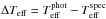 is small, only −41 K, with an rms standard deviation of 73 K. A similar trend was found when applying this relationship to a sample of evolved (subgiant and red giant) stars (Maldonado et al. 2013).
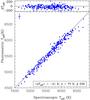 |
Fig. 1 Comparison between our spectroscopically derived Teff and those obtained from (B − V) colours. The upper panel shows the differences between the photometric and the spectroscopic values. Mean uncertainties in the derived temperatures are also shown. |
Evolutionary values of gravities are computed from Hipparcos V magnitudes and the revised parallaxes provided by van Leeuwen (2007). The code PARAM8 (da Silva et al. 2006) has been used together with the new PARSEC isochrones from Bressan et al. (2012). The code also estimates the stellar evolutionary parameters of age, mass, and radius of the star. Our derived spectroscopic Teff and metallicities are used as inputs for PARAM.
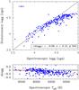 |
Fig. 2 Top panel: comparison between our spectroscopically derived log g values and log g estimates based on Hipparcos parallaxes. Mean uncertainties in log g values are shown. Bottom panel: differences in log g (defined as evolutionary − spectroscopic) as a function of the spectroscopic Teff. A linear fit is shown (dashed line). |
The comparison between the spectroscopic and evolutionary log g values is shown in Fig. 2. Although the differences are small, mean value of only −0.09 (cgs) with a rms deviation of only 0.12 (cgs), it is clear from the figure that evolutionary and spectroscopic values do not always compare well, in particular for high spectroscopic log g values. This discrepancy has already been discussed by several authors (e.g. Sozzetti et al. 2007; Torres et al. 2012; Tsantaki et al. 2013, and references therein). The dependence of Δlog g = log gspec − log gevol is explored in the bottom panel of Fig. 2. Although there is a significant scatter, a trend with the effective temperature can be easily recognised. To our knowledge, the origin of this discrepancy is not known. Several explanations have been put forward, such as departures from LTE or granulation and activity effects, but it might also have an origin related to the relatively small number of Fe ii lines present in the spectra of cool dwarfs (e.g. Tsantaki et al. 2013, and references therein).
The discrepancy between log gspec and log gevol should not affect the other stellar parameters. Temperatures and metallicities derived using the ionisation and excitation equilibrium of iron have been shown to be mostly independent of the adopted surface gravity (Torres et al. 2012). Abundances derived from neutral lines are mostly independent of the surface gravity whilst abundances from single ionised atoms are known to scale with gravity (Gray 2008). We therefore do not expect surface gravity to introduce significant effects on the computation of individual chemical abundances from non-ionised species. In this line, Mortier et al. (2013) computed chemical abundances of 90 stars with transiting exoplanets using spectroscopic log g values and log g estimates derived using the stellar density determined from the light curve. They found that only the abundances from ionised species are significantly affected.
We finally compare our metallicities with those already reported in the literature. Values for the comparison are taken from purely spectroscopic works: MA12 as a consistency double check; the studies of Sousa et al. (2008, 2011a,b, hereafter SO08), which use a similar approach (iron ionisation and excitation conditions) to this paper; and Fischer & Valenti (2005, hereafter VF05) whose parameters are determined by fitting the observed spectra to synthetic models. The comparison is shown in Fig. 3.
Our sample contains 116 stars in common with MA12 and we note that the mean difference between our metallicities and those reported in MA12 is −0.00 dex (σ = 0.08 dex). Fifty-six stars are in common with SO08; the mean difference is +0.00 dex with a rms standard deviation of 0.08 dex. Finally, for the comparison with VF05, we obtain a mean Δ [ Fe/H ] = + 0.02 dex, with σ = 0.08 dex (173 stars in common). In addition, there are no significant differences between our metallicity scale (zero point, slope) and those defined in MA12, SO08, and VF05. We therefore conclude that there are no systematic differences between our derived metallicities and other spectroscopic estimates in the literature.
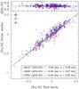 |
Fig. 3 [Fe/H] values, this work vs. literature estimates. Mean uncertainties in the metallicities are shown in the upper left corner of the figure. Top panel: differences between the metallicities derived in this work and the values given in the literature. |
2.6. Abundances
Chemical abundance of individual elements C, O, Na, Mg, Al, Si, S, Ca, Sc, Ti, V, Cr, Mn, Co, Ni, Cu, and Zn are obtained using the 2014 version of the code MOOG9 (Sneden 1973) together with ATLAS9 atmosphere models (Kurucz 1993). Abundances of Sc, Ti, and Cr, were obtained by using lines of the neutral atom and from lines of the single ionised atoms. As it is common in the literature, through this paper we will use X i to refer to the abundances of X computed from lines of the neutral atom, while X ii means abundance of X derived from lines of the single ionised species. The measured equivalent widths of a list of narrow, non-blended lines for each of the aforementioned species are used as inputs. The selected lines are taken from the lists provided by Neves et al. (2009, Table 2), Ramírez et al. (2014, Table 4) for C, O, S, and Cu, and Takeda & Honda (2005, Table 1) in the case of Zn.
For completeness the line list used here is reproduced in Table 3. This table provides the wavelength, excitation potential (EP), and oscillator strength log (gf) for the lines selected in the present work. References are also given. Data for HFS computations are from Ramírez et al. (2014) and are not included in this list.
Wavelength, excitation potential (EP), and oscillator strength log (gf) for the lines selected in the present work.
The O i triplet lines at 777 nm are known to be severely affected by departures from LTE (e.g. Kiselman 1993, 2001). To account for non-LTE effects the prescriptions given by Takeda (2003) were followed. These corrections are essentially determined by the line EWs and the stellar parameters Teff, log g, and ξt. Although they do not contain an explicit dependence on the stellar metallicity, we note that low-metallicity stars are expected to have weaker EWs.
Hyperfine structure (HFS) was taken into account for V i, Co i, and Cu i, using the MOOG driver blends with the wavelengths and relative log (gf) values listed in Ramírez et al. (2014, Table 4). Wavelengths and log (gf) values for the “unresolved line” are from the VALD10 database (Piskunov et al. 1995; Kupka et al. 1999). Another element whose abundance is known to be affected by HFS effects is Mn i. Ramírez et al. (2014) provide HFS data for two Mn i lines. We note, however, a significant offset between the HFS abundance of Mn i derived from the 4502.20 Å line and the abundance obtained from the 6021.80 Å line; while the latter gives abundances that are in agreement with the non-HFS derived ones, HFS abundances derived from the 4502.20 Å line are systematically lower by ~0.4 (e.g. log ϵMnI4502.20 ⊙ = 4.89, log ϵMnI6021.80 ⊙ = 5.46). Because of this difference we prefer not to take into account the HFS corrections for Mn i.
In general, there is a good agreement between the abundances of a given element computed from lines of the neutral atom, and those computed using lines of the single ionised species, although we note a tendency for abundances from neutral ions to be slightly shifted towards higher values for Sc and Ti. This behaviour is not reproduced in the abundances of chromium where Cr i and Cr ii are found to be essentially the same at low values (log ϵCr≲ 5.7), while at higher abundances there seems to be a trend of slightly larger Cr ii abundances.
The solar spectrum provided in the S4N (Allende Prieto et al. 2004) library has been used to derive our own solar reference abundances and are given in Table 4. Our derived solar abundances are in reasonable agreement with recent determinations (e.g. Asplund et al. 2009; Scott et al. 2015b,a; Grevesse et al. 2015), with the exception of Zn I for which we obtain a significantly higher abundance.
Derived solar abundances (log ϵX ⊙), with their corresponding line-to-line scatter error ( ), and number of lines (N).
We have selected four representative stars (HIP 23311 (4848 K), HIP 77408 (5340 K), HIP 113044 (5976 K), and HIP 28767 (6241 K)) that cover the whole Teff range in order to provide an estimate of how the uncertainties in the atmospheric parameters propagate into the abundance calculation. These stars have been selected because their Teff are similar to the 10%, 25%, 75%, and 99% percentiles of the temperature distribution. Abundances for each of these four stars were recomputed using atmosphere models with Teff + ΔTeff, Teff − ΔTeff, and similarly for log g and ξt. Results are given in Table 5. As final uncertainties for the derived abundances, we give the quadratic sum of the uncertainties due to the propagation of the errors in the stellar parameters, plus the line-to-line scatter errors (assuming Gaussian statistics, they are computed as  , where σ is the standard deviation of the derived individual abundances from the N lines). We would like to point out that even these uncertainties should be considered as lower limits, given that the errors in the stellar parameters are only statistical (see Sect. 2.4), and the abundance estimates are affected by systematics which are not taken into account in line-to-line errors (e.g. atomic data or uncertainties in the atmosphere models).
Our obtained final abundances are given in Table 11. It gives the abundances of C I, O I (nLTE corrected), Na I, Mg I, Al I, Si I, S I, Ca I, Sc I, Sc II, Ti I, Ti II, V I (HFS taken into account), Cr I, Cr II Mn I, Co I (HFS taken into account), Ni I, Cu I (HFS considered) and Zn I. They are expressed relative to the solar value, i.e. [ X/H ] = log (NX/NH) − log (NX/NH)⊙. For each star, abundances are given in the first row and uncertainties are given in the second row.
Abundance sensitivities.
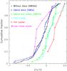 |
Fig. 4 [Fe/H] cumulative frequencies for the different samples studied in this work. The SWP sample is divided into stars hosting exclusively cool distant Jupiters, stars hosting hot close-in planets, and stars with orbiting exclusively low-mass planets. Stars with both low-mass and gas-giant planets are not shown. |
[Fe/H] statistics of the stellar samples.
3. Analysis
3.1. Metallicity distributions
The cumulative distribution function of the metallicity for the different samples analysed in this work is presented in Fig. 4. For guidance some statistical diagnostics are also given in Table 6. We note that statistics corresponding to the different samples of planet hosts should be considered with caution given the small sample size.
The SWP sample has been divided into stars hosting exclusively cool distant Jupiters (semimajor axes, a> 0.1 au, 17 stars), and stars hosting hot close-in planets (a< 0.1 au, 5 stars) given the higher frequency of planets with a≲ 0.07 au shown in the semimajor axis distribution of close-in gas-giant planets, see Wright et al. (2009, Fig. 9) and Currie (2009, Fig. 1). Stars harbouring only low-mass planets (with Mpsini values below ~30 M⊕, 7 stars) have also been considered as a different subsample, since their host stars seem to show different properties with respect to stars hosting gas-giant planets (see Sect. 1). Low-mass and gas-giant planets might coexist. Indeed, two of our stars harbouring a low-mass planet do also host at least one cool Jupiter. A remarkable case is HIP 43587 (55 Cnc), a high-metallicity star (+0.42 dex) harbouring a five planetary system including three hot Jupiters, one low-mass planet, and one cool Jupiter.
As in MA12, we find the metallicity distribution of SWDs and SWODs to be similar. Indeed, a two-sample Kolmogorov-Smirnov test (hereafter K-S test)11 shows that both distributions are quite similar (p-value 51%). Results are given Table 7 which provides the value of the K-S statistic (D), its significance level (p) and the effective size (neff). Further details regarding the K-S test can be found in MA12 (Appendix A).
In MA12 when comparing the metallicity distribution of SWDs and SWODs, a deficit of stars with debris discs at metallicities below approximately −0.1 dex was found. We do not reproduce this result in this work, but we caution that the sample sizes analysed here are smaller than in MA12. Further observations would be required to clarify this point.
We find that the metallicity distribution of SWDPs is clearly different from that of SWDs and similar to that of the stars harbouring cool giant planets. A K-S test confirms that the metallicity distribution of SWDPs differ within a confidence level greater than 98% from those of SWDs and SWODs, while the K-S test reveals that the distribution of SWDPs is very similar to that of cool giant hosts (p-value 81%), see Table 7. Eight SWDPs host at least one low-mass planets. We note that the metallicities of these stars are ≲+0.05 dex with only one exception, HIP 1499.
We therefore conclude that the SWDP sample reproduces the known behaviour of the planet hosts, showing the metal-rich signature only when the planet is a gas-giant (e.g. Gonzalez 1997; Santos et al. 2004; Fischer & Valenti 2005) and not in the case of exclusively low-mass planets (Ghezzi et al. 2010; Mayor et al. 2011; Sousa et al. 2011b; Buchhave et al. 2012).
We note that there seems to be a scarcity of hot Jupiters in SWDPs with only two stars harbouring simultaneously a debris disc and a hot Jupiter. Regarding the metallicity distribution of hot-Jupiters hosts, we find these stars to be more metal-rich than stars hosting exclusively cool distant planets, as already noted in MA12. However, we caution that the K-S test produces inconclusive results; the probability of both samples showing similar distributions is 20%. This trend was previously discussed in Gonzalez (1998), Queloz et al. (2000), Sozzetti (2004); and more recently in Adibekyan et al. (2013). A more extensive discussion is provided in Appendix B.
Results of the K-S tests performed in this work.
3.2. Other chemical signatures
In order to find differences in the abundances of other chemical elements besides iron, the cumulative distribution [X/Fe] comparing the abundances between SWDs and SWODs is shown in Fig. 5. Some statistical diagnostics are also presented in Table 8, where the results of a K-S test for each ion are also listed. For each star, abundances with large errors (uncertainties greater than 0.30 dex) were excluded from this exercise.
Similar behaviour between stars with debris discs and stars without known discs is found. From the 20 chemical species analysed, the K-S accepts the null hypothesis (i.e. SWD and SWOD distributions being drawn from the same parent population) in 19. The only exception is the Cu i abundance for which the K-S test returns a probability of the null hypothesis lower than 0.01. We also note that the K-S probability corresponding to the Zn i is significantly low, of the order of 0.04 (although the null hypothesis is not rejected). Nevertheless, we caution that abundances of Cu i and Zn i are based on only two lines. Furthermore Cu i abundance is severely affected by HFS effects.
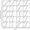 |
Fig. 5 [X/Fe] cumulative fraction of SWDs (blue dashed line) and SWODs (black continuous line). |
Comparison between the elemental abundances of SWODs and SWDs.
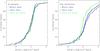 |
Fig. 6 Histogram of [X/Fe]-TC slopes derived when all elements (volatiles plus refractories) are taken into account (left) and when only refractories are considered (right). |
3.3. [X/Fe]-TC trends in SWDPs
Another way of searching for chemical differences is to study possible trends between the abundances and the elemental condensation temperature, TC. For each of the stars analysed in this work, the [X/Fe] trend as a function of the TC was obtained. Values of TC correspond to a 50% equilibrium condensation temperature for a solar system composition gas (Lodders 2003). Each trend is characterised by a linear fit, weighting each abundance by its corresponding uncertainty12. Given the relatively low number of volatile elements considered in this work and the fact that their abundances are in general more difficult to obtain accurately (few lines that can be blended, non-LTE effects), we compute the slope of the [X/Fe] vs. TC fit considering all refractory and volatile elements ( -slope), and considering only refractories (
 -slope). Following the discussion in Ramírez et al. (2010, Sect. 5.3) we consider as volatile those elements with TC lower than 900 K, namely C, O, S, and Zn.
The cumulative distribution functions of -slope, and -slope are shown in Fig. 6 for the SWOD sample (black crosses), the SWD sample (blue asterisks), and the SWDP sample (green triangles). The -slope distribution is in the left panel whilst the distribution of -slope is shown in the right panel. Several interesting trends emerge from this figure. First, when considering the cumulative distribution of -slope (left), all the samples considered here (SWDs, SWODs, and SWDPs) show similar distributions. However, if we consider only refractory elements (right), the SWDP sample seems to behave in a different way with respect to the SWOD and SWD samples. It can be seen that SWDPs seem to have slightly more negative values of -slope than the other two samples, in particular at slopes above − 1 × 10⁻⁴ dex/K. Statistically, this different behaviour of SWDPs in -slope seems to be significant with K-S p-probabilities of the order of ~0.03 when comparing SWDPs and SWODs, and of the order of ~0.01 when SWDPs are compared to SWDs.
Results of the ⟨[ X/Fe ] ⟩ − TC linear fits.
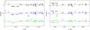 |
Fig. 7 ⟨[ X/Fe ] ⟩ − TC trends for the SWOD, SWD, and SWDP samples when all elements (volatiles and refractories) are taken into account (left) and when only refractories are considered (right). For the sake of clarity, an offset of −0.50 dex was applied between the samples. Unweighted fits are shown by continuous lines, while weighted fits are plotted in dashed lines. For guidance, the derived slopes from the unweighted fits are shown in the plots (units of 10-5 dex/K). |
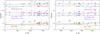 |
Fig. 8 ⟨[ X/Fe ] ⟩ − TC trends for planet host stars. The stars are divided into six categories, three corresponding to stars with known planets but no debris discs, namely, stars hosting cool Jupiters (light-blue open circles), low-mass planet hosts (pink earth symbols), and stars hosting hot Jupiters (red filled circles). The SWDP sample is divided into the same categories: stars with debris discs and cool Jupiters (pink filled squares), debris discs and low-mass planets (cyan filled stars), and stars harbouring debris discs and hot Jupiters (light green asterisks). Each planet host subsample is shown against its corresponding SWDP subsample (e.g. stars with cool Jupiters vs. stars with discs and cool Jupiters) with an offset of −0.15 between the samples for the sake of clarity. The offset between the samples of cool, low-mass, and hot Jupiters hosts is −0.75. Unweighted fits are shown by continuous lines, while weighted fits are plotted in dashed lines. For guidance, the derived slopes from the unweighted fits are shown in the plots (units of 10-5 dex/K). The left panel shows the ⟨[ X/Fe ] ⟩ − TC trends when all elements (volatiles and refractories) are taken into account whilst the right one shows the ⟨[ X/Fe ] ⟩ − TC trends when only refractories are considered. |
Mean abundances for each of the samples (SWDS, SWODs, SWDPs) were also computed, and -slope, -slope derived. As errors we considered the star-to-star scatter. As explained above, each trend is characterised by a linear fit. Two different fits were performed, one weighting each element by its corresponding error and another without weighting. The corresponding plots are shown in Fig. 7, and a summary of the fits is shown in Table 9. To give a significance for the derived slopes a Monte Carlo simulation was carried out. We created 10 000 series of simulated random abundances and errors, keeping the media and the standard deviation of the original data. For each series of simulated data the corresponding TC-slope was derived. Assuming that the distribution of the simulated slopes follows a Gaussian function we then compute the probability that the simulated slope takes the value found when fitting the original data.
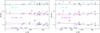 |
Fig. 9 ⟨[ X/Fe ] ⟩ − TC trends for stars with cool Jupiters (light blue open circles), stars with exclusively low-mass planets (pink earth symbols), and stars with low-mass planets and cool Jupiters (purple open diamonds). For the sake of clarity, an offset of −0.75 dex was applied between the samples. For guidance, the derived slopes from the unweighted fits are shown in the plots (units of 10-5 dex/K). The left panel shows the ⟨[ X/Fe ] ⟩ − TC trends when all elements (volatiles and refractories) are taken into account, whilst the right panel shows the ⟨[ X/Fe ] ⟩ − TC trends when only refractories are considered. |
In the left panel, when all elements (volatiles and refractories) are considered, the unweighted fits (continuous line) reveal a different behaviour of SWDPs with respect to the samples of stars without known planetary companions. The SWDP sample shows a slightly positive slope while the slope of the SWODs and SWDs seems to be negative. However, the analysis of the significance of the slopes shows the need for caution since these trends seem to be tentative (see Table 9). In fact, when the linear fit is done by weighting each element by its corresponding error (dashed lines) the suggested trends tend to disappear and SWODs, SWDs, and SWDPs seem to show similar positive slopes. The significance of the weighted fits are moderate (probability of the slope “being by chance” ≤23%).
When only refractory elements are considered (right panel), in the unweighted fits (continuous line) SWDs and SWODs show a positive trend, whilst SWDPs follow a slightly negative tendency. In this case, the different sign of SWDPs with respect to SWDs and SWODs is also present in the weighted fits (dashed lines). The significance of the -slope fits are in all cases (weighted and weighted fits) moderate (probability of the slope “being by chance” between 8 and 20%) with the only exception of the unweighted fit of the SWDP sample (62%).
3.4. Comparison with planet hosts
The ⟨[ X/Fe ] ⟩ − TC of the SWDP sample can also be compared with the results from our sample of stars hosting cool giant planets, hot close-in Jupiters, and low-mass planets. For this purpose the SWDP sample has been divided into stars with discs and cool giant planets, stars with discs and low-mass planets, and stars harbouring discs and hot Jupiters. The corresponding trends are shown in Fig. 8 where each planet host subsample (cool, low-mass, or hot planets) is compared with its corresponding SWDP subsample (disc and cool, disc and low-mass, disc and hot planets). The fits results are given in Table 9. Several conclusions can be drawn from this analysis.
We first note that SWDP seem to behave in a similar way to stars with known planets. It can be easily seen in the left panel of Fig. 8 (i.e. when all the elements are considered) that this statement holds for stars hosting cool Jupiters and low-mass planets. A similar behaviour is found when only refractory elements are considered (right panel).
Second, there seems to be a hint that low-mass planet hosts show a different behaviour in the unweighted fits in comparison with stars with gas-giant planets. This is true for both (low-mass planet hosts show negative slopes whilst cool Jupiters hosts show positive slopes) and  analysis (positive slopes for stars with low-mass planets, negatives for stars with cool Jupiters). This trend also seems to be present in the weighted fits for all elements.
We note at this point that we have classified as stars with low-mass planets those stars hosting exclusively these kind of planets (i.e. without giant Jupiters). We have two stars harbouring simultaneously low-mass and cool Jupiters13. Their ![Mathematical equation: \hbox{$\left<[{\rm X/Fe}]\right>-T^{\rm all}_{\rm C}$}](/articles/aa/full_html/2015/07/aa25764-15/aa25764-15-eq87.png) trends are compared with cool Jupiters hosts and low-mass planets hosts in Fig. 9. It can be seen that stars with low-mass and cool planets do not seem to behave like stars with exclusively low-mass planets. In particular, in the analysis, where stars with low-mass and cool planets show a clear negative slope whilst stars with only low-mass planets show a positive one.
trends are compared with cool Jupiters hosts and low-mass planets hosts in Fig. 9. It can be seen that stars with low-mass and cool planets do not seem to behave like stars with exclusively low-mass planets. In particular, in the analysis, where stars with low-mass and cool planets show a clear negative slope whilst stars with only low-mass planets show a positive one.
Setting together the results from the analysis of Figs. 7, 8, and 9 it seems that the slopes in the unweighted analysis tend to be negative, unless the stars host a Jupiter (stars with cool Jupiters, hot Jupiters, and debris plus cool Jupiters). On the other hand, in the unweighted fits the slopes tend to be positive in all samples, but negative in those samples hosting a cool gas-giant planet (stars with cool Jupiters, with debris plus cool Jupiters, with low-mass planets and cool Jupiters, and also stars with debris and hot Jupiters). In other words, the samples of stars with cool giant planets seem to behave in a different way with respect to the non-planet hosts samples.
Finally, and despite our low statistics (only five stars), it is worth mentioning that the sample of stars hosting hot Jupiters (Fig. 8) shows in all cases (all elements, only refractories, weighted, and unweighted fits) a clear positive slope (only SWDs and SWODs in the unweighted analysis show positive slopes of similar values). There is, however, a clear disagreement between stars with hot Jupiters and the behaviour of the stars simultaneously hosting a debris discs and hot Jupiters. The reasons for this discrepancy can be found in the low number of stars in both samples, but perhaps also because of the clearly different mean abundance of copper. We also note that none of the stars in the hot Jupiters host sample has a reliable oxygen abundance.
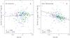 |
Fig. 10
|
4. Discussion
In a recent work Meléndez et al. (2009, hereafter ME09), report a deficit of refractory elements in the Sun with respect to other solar twins. After discussing several possible origins, the authors conclude that the most likely explanation is related to the formation of planetary systems like our own, in particular to the formation of rocky low-mass planets. A similar conclusion was reached by Ramírez et al. (2009), and Gonzalez et al. (2010). Although very appealing, the ME09 hypothesis has been challenged. Other works point instead towards Galactic chemical evolution (GCE) effects as the cause of the detected small chemical depletions (González Hernández et al. 2010, 2013) or towards an age/Galactic birth place explanation (Adibekyan et al. 2014).
In the previous section several interesting (although some certainly tentative) trends in planet hosts have been found: i) there seem to be no chemical differences between SWDs and SWODs; ii) SWDPs behave as stars with planets; iii) stars with low-mass planets do not seem to behave in a different way with respect to the SWD and SWOD samples; iv) the samples of stars with cool Jupiters seem to be the ones that might follow a different trend with respect to the SWD and SWOD samples; and v) stars hosting hot Jupiters seem to show positive slopes. At this point, in order to understand the origin and significance of these findings, two main questions should be discussed: might the ⟨[ X/Fe ] ⟩ − TC trends be influenced by effects of metallicity, age, or Galactocentric distance? And do these ⟨[ X/Fe ] ⟩ − TC trends fit in the framework of ME09 hypothesis?
4.1. Age, metallicity, and Galactocentric distance effects
Abundance patterns may be affected by GCE effects. González Hernández et al. (2013) account for these effects by fitting straight lines to the [X/Fe] vs. [Fe/H] plots. The obtained trends are then removed from the original [X/Fe] data. Ramírez et al. (2014), however, argue that correcting from GCE effects in this manner may prevent us from finding elemental depletions due to planet formation.
A way to disentangle the effects of chemical evolution from those related to fractionated accretion is to analyse the dependence of the TC-slope as a function of the stellar metallicity. When considering all elements, abundances of C i and O i tend to rise towards lower metallicities, producing negative slopes in the abundance vs. TC plot for stars with low metallicities (e.g. Ecuvillon et al. 2006, and references therein). The -slope vs. [Fe/H] plot for our stars is explored in Fig. 10 (left) where it can be seen that no clear trend is found. We recall at this point, that our abundance ratios as a function of the stellar metallicity are consistent with previous works (see Appendix C).
However, when considering the -slope (Fig. 10, right) a trend of decreasing slopes towards high metallicities seems to be present (negative in this case since the abundances of C i and O i are not considered). A Spearman’s correlation test shows that the correlation, although moderate (ρ = − 0.50), seems to be highly significant (prob ~10-17). The possibility that GCE effects affect our abundance analysis can therefore not be ruled out.
The observed correlation between the presence of gas-giant planets and enhanced metallicity has been widely debated in the context of two different scenarios of planet formation, core-accretion and disc instabilities. Little attention has been paid to other lines of argument. In particular, Haywood (2009) suggested a possible inner-disc origin of the planet hosts as an explanation. Recently, Adibekyan et al. (2014) found correlations between the TC-slope and the stellar age, the surface gravity, and the mean Galactocentric distance of the star, Rmean, suggesting that the age and the Galactic birth place (and not the presence of planets) are likely the parameters that determine the chemical properties of the stars.
A similar search for correlations was performed in our sample of planet hosts. Stellar ages from MA12 (or derived in the same manner) were used. These ages are based on the  activity index following the prescriptions of Mamajek & Hillenbrand (2008). As a consistency check, the TC-age relationship was also studied by using the isochrone ages provided by the PARAM code (da Silva et al. 2006). Regarding the Galactic parameters, values for the mean Galactocentric radii were taken from Casagrande et al. (2011).
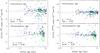 |
Fig. 11
|
The results (see Fig. 11) show a weak but significant correlation with the stellar age. Results from a Spearman’s correlation test provide ρ = − 0.02, prob ~0.74 for -isochrone age; ρ = 0.14, prob ~0.03 for -isochrone age; ρ = 0.12, prob ~0.09 for -chromospheric age; and ρ = − 0.15, prob ~0.03 for -chromospheric age. Our results confirm the findings by Adibekyan et al. (2014) in the sense that a correlation between TC-slope and age is likely to be present, although we find it to be relatively weak.
We find, however, no clear correlation between TC-slope and Rmean in disagreement with Adibekyan et al. (2014), although these authors only suggest tentative evidence (and not a strong correlation). Furthermore, our abundance ratios are not corrected from possible GCE effects. The plot of TC-slope vs. Rmean is shown in Fig. 12.
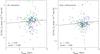 |
Fig. 12
|
In order to test whether our results are affected or not by GCE effects, our abundances were corrected following the procedure of González Hernández et al. (2013), although we fitted the [X/H] vs. [Fe/H] plane (see Fig. C.1) instead of the [X/Fe]-[Fe/H] plane (our Fig. C.2). The reason for doing so is the larger scatter found in the [X/Fe] vs. metallicity plane probably due to the large number of stars, as well as the broader range of stellar parameters covered in this work. Except for the expected trend of higher [X/H] values as we move towards higher metallicities and a larger scatter in the elements whose abundances are based on a smaller number of lines, no other significant trends are revealed by the [X/H] vs. [Fe/H] plots.
As before, values of -slope and -slope were computed for each individual star and a search for correlations with the stellar radii, metallicity, age, and mean Galactocentric distance was performed. A summary of the results from the Spearman’s correlation tests are given in Table 10. It can be seen that our results do not change significantly. The GCE-corrected -slope does not show any clear correlation with any of the mentioned stellar properties. Regarding the GCE-corrected -slope, it shows a weak but significant correlation with the stellar age (but only when considering chromospheric ages) and a moderate (ρ = 0.54) significant correlation with the stellar radius. These two correlations were also found without correcting for GCE effects.
Results from the Spearman’s correlation tests between the GCE effects corrected TC-slope and different stellar properties.
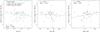 |
Fig. 13
|
4.2. Abundance patterns and the presence of discs and planets
The first two observational results of this work, the lack of a chemical difference in SWDs with respect to SWODs and the fact that SWDPs behave in a similar way to stars with planets (showing different ⟨[ X/Fe ] ⟩ − TC trends when the planet is a cool giant, but not when the star hosts exclusively low-mass planets), indicate that the factor that reveals the chemical behaviour of the corresponding star is the presence of planets, and not the presence of discs.
This was first established in MA12, although only on the basis of metallicity distributions. This result fits well in the framework of the core-accretion model of planet formation (e.g. Pollack et al. 1996; Ida & Lin 2004; Hubickyj et al. 2005; Mordasini et al. 2009, 2012), where the conditions for the formation of debris are more easily met than the conditions for the formation of gas-giant planets.
Maldonado et al. (2012) noticed that among the SWDP sample there was a significant fraction of stars hosting low-mass planets, mainly in multiplanet systems. Wyatt et al. (2012) suggested that stars with low-mass planets might be more likely to have detectable debris discs, arguing that the same processes that lead to the formation of low-mass planets may result in high levels of outer debris. The lack of a metallicity enhancement in SWDs with respect to SWODs, and the lower metallicities of stars with low-mass planets with respect to stars hosting gas-giant planets do certainly support this hypothesis. In fact, additional evidence of the correlation between the presence of dust, low-mass planets, and lower stellar metallicities has been recently found by Marshall et al. (2014). However, we caution that there are several biases that might prevent us from finding a clear statistically significant correlation (Moro-Martín et al. 2015).
In the framework of the ME09 hypothesis, stars hosting low-mass planets should show negative ⟨[ X/Fe ] ⟩ − TC slopes. Since low-mass planets might be common in SWDS, a search for correlations between the properties of the dust and -slope of the stars with discs (SWDs and SWDPs) was performed. Basic physical parameters of the discs, fractional dust luminosity Ldust/L⋆, dust temperature Tdust, and disc radius Rdisc are taken from Eiroa et al. (2013) when possible since it constitutes a homogeneous database of debris disc parameters. Otherwise, these values are taken from the literature (see MA12 and references therein). The results from the statistical tests (see Fig. 13) show no clear correlation between the properties of the discs and the chemical composition of the star. In addition, no significant difference in any of the considered properties between the stars with debris discs and cool Jupiters and the SWDs has been found14.
We should note at this point that the fact that we do not find a clear chemical fingerprint of low-mass planet formation in the SWDs as a whole does not contradict the idea that low-mass planets and discs might be a correlated phenomenon. First, the ME09 interpretation needs to be confirmed. Second, there are several biases in our analysis since the values of the dust properties are taken from different sources. Furthermore, values of the disc radius are usually computed by assuming black-body emission which is known to underestimate the radial distance of the dust from the star by a factor of up to four around G stars (Marshall et al. 2011; Wyatt et al. 2012). Finally, the chemical depletions we are looking for are small (~0.08 dex) and in most cases have been found by a differential analysis between stars with very similar parameters (and mostly solar twins). A more detailed differential analysis of individual SWD stars with respect to their corresponding SWODs twins is deferred to a forthcoming paper.
The second observational result of this work, i.e the slopes of stars hosting low-mass planets, does not seem to support the ME09 hypothesis. We do find that low-mass planet hosts show negative slopes, but only when all elements are considered and, more importantly, that SWDs and SWODs also show negative slopes in this case. Moreover, our data suggests that the stars hosting cool Jupiters are the ones that show a different ⟨[ X/Fe ] ⟩ − TC trend with respect to the non-planet host samples. This is true when all elements are considered and also when the analysis is restricted to refractory elements. In this case, the slopes of the samples hosting cool Jupiters are negative.
Finally, the positive slope in stars hosting hot Jupiters should be interpreted with caution given the small size of our sample, but also because SWODs and SWDs show clear positive slopes in the analysis. We simply note that a significant positive slope in the framework of the ME09 hypothesis can be interpreted as an indication that low-mass planets are not present.
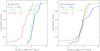 |
Fig. 14 Histogram of [X/Fe]-TC slopes for all planet hosts as a function of the stellar radius when all elements (volatiles plus refractories) are taken into account (left) and when only refractories are considered (right). |
4.3. Signatures of pollution
A correlation between elemental abundances and condensation temperature is a natural prediction of the self-enrichment hypothesis for the gas-giant planet metallicity correlation (Gonzalez 1997) because the accretion of material by a star is expected to occur close to the star, a high temperature environment. Therefore, refractory elements might be preferentially added when compared to volatile elements. The abundance pattern of hotter dwarfs constitutes an important test for this scenario. These stars are known to have narrower convective envelopes (i.e. to experience less mixing) and, therefore, the chemical signature in the ⟨[ X/Fe ] ⟩ − TC trend suggested in planet hosts should be more significant in these stars than in late-type stars.
The stellar radii is used here as a proxy of the convective envelope size. In main-sequence stars it is larger for early-type stars, whilst it diminishes for late-type stars. The stellar radii have been computed as explained in Sect. 2.5. Our sample of planet hosts, i.e. the sum of the SWP and the SWDP samples (irrespective of the planet’s type) has been divided into three categories according to their radii: i) F-stars, with R⋆> 1.12R⊙; ii) G-stars, with 0.91 R⊙<R⋆< 1.12R⊙; and iii) K-stars, with 0.91 R⊙<R⋆ (see Gray 2008, Table B.1).
The cumulative distribution functions of -slope and -slope of these three subsamples are compared in Fig. 14. It is clear from this figure that the only significant difference is in the distribution of -slope, where K-stars show larger negative slopes than the other two samples (with K-S p-values of ~10-5 when comparing K with F stars, and ~10-4 when comparing K with G stars). This point argues against the pollution hypothesis. When considering all elements, negative slopes are signatures of a possible deficit of refractory elements with respect to volatiles. If this deficit is not primordial, but rather is due to the later accretion of refractory-depleted material, stars with narrower convective zones (early F) should show higher levels of depletion, or in other words, larger negative slopes. Furthermore, no difference in the -slope distributions is found between the F, G, and K star samples. And thus the pollution hypothesis is not sustained with the data at hand.
4.4. Trends with planetary properties
Finally, the stellar [X/Fe] vs. -slopes are plotted in Fig. 15 as a function of the planetary properties, minimum mass, period, semimajor axis, and eccentricity. No clear trend has been identified, in agreement with previous works (e.g. Ecuvillon et al. 2006).
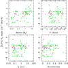 |
Fig. 15
|
5. Summary
In this work a detailed chemical analysis of stars with dusty debris discs has been presented. Their chemical abundances have been compared to those of stars with planets, stars harbouring debris discs and planets, and stars with neither debris nor planets.
No clear difference has been found in metallicity, individual abundances, or ⟨[ X/Fe ] ⟩ − TC trends between SWDs and SWODs. The behaviour of SWDPs seems to be driven by the type of planet (cool Jupiter or low-mass planet). This is in agreement with the core-accretion model for planet formation in which the conditions required to form debris discs are more easily met than the conditions to form gas-giant planets. The fact that SWDs like stars with low-mass planets do not show metal enhancement might indicate a correlation between both phenomena. Giant planets in eccentric orbits might produce dynamical instabilities that can clear out the inner and outer parts of a debris disc, which might explain the lack of a clear correlation between debris discs and more massive planets.
We find tentative different behaviours in ⟨[ X/Fe ] ⟩ − TC trends between the samples of stars with planets and the samples of stars without planets. Stars with cool giant planets seem to behave in a different way with respect to the samples of stars without planets. This result holds independently of whether all elements or only refractories are considered. In particular, when only refractory elements are considered stars with cool planets show negative slopes. We find that stars with exclusively low-mass planets behave as the non-planet hosts do. Despite our small sample size, stars hosting exclusively close-in giant planets seem to show higher metallicities than stars harbouring more distant planets. Furthermore, they show positive TC slopes although this trend should be investigated further.
Finally, we have some words of caution about the interpretation of the negative slopes as a signature of planet formation since the derived trends show relatively low statistical significance levels and the TC-slopes show a moderate but significant correlation with the stellar metallicity. Even after correction for these possible effects, a relatively weak correlation between TC-slope with the stellar age and a moderate one with the stellar radius remains.
Online material
Spectroscopic parameters with uncertainties for the stars measured in this work.
Wavelength, excitation potential (EP), and oscillator strength log (gf) for the lines selected in the present work.
Derived abundances [X/H].
Appendix A: Data from the ESO Science Archive Facility
ESO/ST-ECF Science Archive Facility data used in this work.
To give full credit to data used in this paper coming from the ESO/ST-ECF Science Archive Facility15, and the pipeline processed FEROS and HARPS data archive16, the corresponding ESO programme IDs are listed in Table A.1.
Appendix B: The metallicity distribution of stars with cool and hot Jupiters
As seen in Sect. 3.1 we find that stars hosting close-in hot Jupiters tend to show higher metallicities than stars hosting more distant planets. Given the small number of stars considered in this work we performed an additional check by considering the metallicity distribution of all stars known to harbour planets as listed17 in the Extrasolar Planets Encyclopaedia (Schneider et al. 2011) and the Exoplanet Orbit Database (Wright et al. 2011) databases. All planet hosts with available values of planetary mass, semimajor axis, and metallicity were considered. Stars with low-mass planets (MPsini< 30 M⊕) were discarded. No further selection criteria were applied. Stars with multiple planets are classified as “hot” if at least one of the planets has a semimajor axis smaller than 0.1 au. The resulting metallicity distributions are shown in Fig. B.1, while some statistical diagnostics are given in Table B.1.
[Fe/H] statistics of cool/hot Jupiter host stellar samples.
We can see from the figure that at high metallicities (greater than +0.0/+0.1 dex) the metallicity distributions of stars hosting cool and stars hosting hot planets are nearly the same. However, they differ at low-metallicities; the distribution of hot Jupiters is slightly shifted towards higher metallicities. We also note that there are no hot Jupiters harbouring stars with metallicities below −0.50/−0.60 dex, while cool Jupiters can be found around stars as metal-poor as −1.00 dex. A K-S test shows that we cannot rule out the possibility of both distributions (hot/cool stellar hosts) being drawn from the same parent population. However, the derived p-values are very low, only 0.15 when data from exoplanets.org is considered (neff ~ 115, D ~ 0.11) and 0.06 if the data from exoplanet.eu is employed (neff ~ 127, D ~ 0.12).
These results are in agreement with previous works (see references in Sect. 3.1) that point towards a paucity of short period planets around metal-poor stars. While this trend could in principle suggest a metallicity dependency of migration rates, further monitoring of metal-poor stars are required to confirm it (Sozzetti 2004).
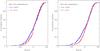 |
Fig. B.1 Histogram of [Fe/H] cumulative frequencies for all stars with cool (blue) and hot (red) Jupiters listed in exoplanets.org (left) and exoplanet.eu (right). |
Appendix C: Abundance ratios as a function of stellar metallicity
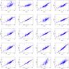 |
Fig. C.1 Chemical abundance ratios of [X/H] as a function of the stellar metallicity. The red line shows the best linear fit. |
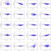 |
Fig. C.2 Chemical abundance ratios of [X/Fe] as a function of the stellar metallicity. The red line shows the best linear fit. |
As listed on September 18, 2014, in the Extrasolar Planets Encyclopedia.
Performed with the IDL Astronomy User’s Library routine kstwo, see http://idlastro.gsfc.nasa.gov/
Our abundances are given with respect to the Sun, while other works compute the abundance difference Star − Sun (e.g. Meléndez et al. 2009; González Hernández et al. 2013).
HIP 43587 is not considered since it also hosts several hot Jupiters.
There are very few discs and low-mass/hot Jupiter planets hosts with data for performing a K-S test. Stars with lower/upper limits have not been considered in the statistics.
Up to June 14, 2014.
Acknowledgments
J.M. acknowledges support from the Italian Ministry of Education, University, and Research through the Premiale HARPS-N research project under grant Ricerca di pianeti intorno a stelle di piccola massa. Additional funding from the Spanish Ministerio de Economía y Competitividad under grant AYA2011-26202 is also acknowledged. E.V. acknowledges support from the Spanish Ministerio de Economía y Competitividad under grant AYA2013-45347P. The authors would like to thank Robert. L. Kurucz, Sergio Sousa, Yoichi Takeda, Chris Sneden, and Léo Girardi, for making their codes publicly available. Jean Schneider is also acknowledged for maintaining the Extrasolar Planets Encyclopedia. This research has also made use of the Exoplanet Orbit Database and the Exoplanet Data Explorer at exoplanets.org, the VizieR catalogue access tool, CDS, Strasbourg, France, as well as the NASA’s Astrophysics Data System Bibliographic Services.
References
- Adibekyan, V. Z., Figueira, P., Santos, N. C., et al. 2013, A&A, 560, A51 [NASA ADS] [CrossRef] [EDP Sciences] [Google Scholar]
- Adibekyan, V. Z., González Hernández, J. I., Delgado Mena, E., et al. 2014, A&A, 564, L15 [NASA ADS] [CrossRef] [EDP Sciences] [Google Scholar]
- Allen de Prieto, C., Barklem, P. S., Lambert, D. L., & Cunha, K. 2004, A&A, 420, 183 [NASA ADS] [CrossRef] [EDP Sciences] [Google Scholar]
- Asplund, M., Grevesse, N., Sauval, A. J., & Scott, P. 2009, ARA&A, 47, 481 [NASA ADS] [CrossRef] [Google Scholar]
- Aumann, H. H., Beichman, C. A., Gillett, F. C., et al. 1984, ApJ, 278, L23 [NASA ADS] [CrossRef] [Google Scholar]
- Backman, D. E., & Paresce, F. 1993, in Protostars and Planets III, eds. E. H. Levy, & J. I. Lunine, 1253 [Google Scholar]
- Beichman, C. A., Bryden, G., Rieke, G. H., et al. 2005, ApJ, 622, 1160 [NASA ADS] [CrossRef] [Google Scholar]
- Boisse, I., Pepe, F., Perrier, C., et al. 2012, A&A, 545, A55 [NASA ADS] [CrossRef] [EDP Sciences] [Google Scholar]
- Bonsor, A., Kennedy, G. M., Wyatt, M. C., Johnson, J. A., & Sibthorpe, B. 2014, MNRAS, 437, 3288 [NASA ADS] [CrossRef] [Google Scholar]
- Bressan, A., Marigo, P., Girardi, L., et al. 2012, MNRAS, 427, 127 [NASA ADS] [CrossRef] [Google Scholar]
- Bryden, G., Beichman, C. A., Carpenter, J. M., et al. 2009, ApJ, 705, 1226 [NASA ADS] [CrossRef] [Google Scholar]
- Buchhave, L. A., Latham, D. W., Johansen, A., et al. 2012, Nature, 486, 375 [NASA ADS] [Google Scholar]
- Casagrande, L., Ramírez, I., Meléndez, J., Bessell, M., & Asplund, M. 2010, A&A, 512, A54 [NASA ADS] [CrossRef] [EDP Sciences] [Google Scholar]
- Casagrande, L., Schönrich, R., Asplund, M., et al. 2011, A&A, 530, A138 [NASA ADS] [CrossRef] [EDP Sciences] [Google Scholar]
- Cassan, A., Kubas, D., Beaulieu, J.-P., et al. 2012, Nature, 481, 167 [NASA ADS] [CrossRef] [Google Scholar]
- Chavero, C., Gómez, M., Whitney, B. A., & Saffe, C. 2006, A&A, 452, 921 [NASA ADS] [CrossRef] [EDP Sciences] [Google Scholar]
- Currie, T. 2009, ApJ, 694, L171 [NASA ADS] [CrossRef] [Google Scholar]
- da Silva, L., Girardi, L., Pasquini, L., et al. 2006, A&A, 458, 609 [NASA ADS] [CrossRef] [EDP Sciences] [Google Scholar]
- Ecuvillon, A., Israelian, G., Santos, N. C., Mayor, M., & Gilli, G. 2006, A&A, 449, 809 [NASA ADS] [CrossRef] [EDP Sciences] [Google Scholar]
- Eiroa, C., Fedele, D., Maldonado, J., et al. 2010, A&A, 518, L131 [NASA ADS] [CrossRef] [EDP Sciences] [Google Scholar]
- Eiroa, C., Marshall, J. P., Mora, A., et al. 2013, A&A, 555, A11 [NASA ADS] [CrossRef] [EDP Sciences] [Google Scholar]
- Fischer, D. A., & Valenti, J. 2005, ApJ, 622, 1102 [NASA ADS] [CrossRef] [Google Scholar]
- Frandsen, S., & Lindberg, B. 1999, in Astrophysics with the NOT, eds. H. Karttunen, & V. Piirola, 71 [Google Scholar]
- Gänsicke, B. T., Koester, D., Farihi, J., et al. 2012, MNRAS, 424, 333 [NASA ADS] [CrossRef] [Google Scholar]
- Ghezzi, L., Cunha, K., Smith, V. V., et al. 2010, ApJ, 720, 1290 [NASA ADS] [CrossRef] [Google Scholar]
- Gonzalez, G. 1997, MNRAS, 285, 403 [NASA ADS] [CrossRef] [Google Scholar]
- Gonzalez, G. 1998, A&A, 334, 221 [NASA ADS] [Google Scholar]
- Gonzalez, G. 2011, MNRAS, 416, L80 [NASA ADS] [CrossRef] [Google Scholar]
- Gonzalez, G., Carlson, M. K., & Tobin, R. W. 2010, MNRAS, 407, 314 [NASA ADS] [CrossRef] [Google Scholar]
- GonzálezHernández, J. I., Israelian, G., Santos, N. C., et al. 2010, ApJ, 720, 1592 [NASA ADS] [CrossRef] [Google Scholar]
- GonzálezHernández, J. I., Delgado-Mena, E., Sousa, S. G., et al. 2013, A&A, 552, A6 [NASA ADS] [CrossRef] [EDP Sciences] [Google Scholar]
- Gratton, R. G., Bonanno, G., Bruno, P., et al. 2001, Exp. Astron. 12, 107 [NASA ADS] [CrossRef] [Google Scholar]
- Gray, D. F. 2008, The Observation and Analysis of Stellar Photospheres (Cambridge: Cambridge University Press) [Google Scholar]
- Greaves, J. S., Fischer, D. A., & Wyatt, M. C. 2006, MNRAS, 366, 283 [NASA ADS] [CrossRef] [Google Scholar]
- Grevesse, N., Scott, P., Asplund, M., & Sauval, A. J. 2015, A&A, 573, A27 [NASA ADS] [CrossRef] [EDP Sciences] [Google Scholar]
- Haywood, M. 2009, ApJ, 698, L1 [NASA ADS] [CrossRef] [Google Scholar]
- Hubickyj, O., Bodenheimer, P., & Lissauer, J. J. 2005, Icarus, 179, 415 [NASA ADS] [CrossRef] [Google Scholar]
- Ida, S., & Lin, D. N. C. 2004, ApJ, 616, 567 [NASA ADS] [CrossRef] [MathSciNet] [Google Scholar]
- Jewitt, D., Moro-Martìn, A., & Lacerda, P. 2009, in The Kuiper Belt and Other Debris Disks, eds. H. A. Thronson, M. Stiavelli, & A. Tielens, 53 [Google Scholar]
- Kiselman, D. 1993, A&A, 275, 269 [Google Scholar]
- Kiselman, D. 2001, New A Rev., 45, 559 [Google Scholar]
- Kóspál, Á., Ardila, D. R., Moór, A., & Ábrahám, P. 2009, ApJ, 700, L73 [NASA ADS] [CrossRef] [Google Scholar]
- Kupka, F., Piskunov, N., Ryabchikova, T. A., Stempels, H. C., & Weiss, W. W. 1999, A&AS, 138, 119 [NASA ADS] [CrossRef] [EDP Sciences] [MathSciNet] [PubMed] [Google Scholar]
- Kurucz, R. 1993, ATLAS9 Stellar Atmosphere Programs and 2 km/s grid, Kurucz CD-ROM No. 13 (Cambridge, Mass.: Smithsonian Astrophysical Observatory) [Google Scholar]
- Lestrade, J.-F., Matthews, B. C., Sibthorpe, B., et al. 2012, A&A, 548, A86 [NASA ADS] [CrossRef] [EDP Sciences] [Google Scholar]
- Lodders, K. 2003, ApJ, 591, 1220 [NASA ADS] [CrossRef] [Google Scholar]
- Luhman, K. L., Patten, B. M., Marengo, M., et al. 2007, ApJ, 654, 570 [NASA ADS] [CrossRef] [Google Scholar]
- Maldonado, J., Martínez-Arnáiz, R. M., Eiroa, C., Montes, D., & Montesinos, B. 2010, A&A, 521, A12 [NASA ADS] [CrossRef] [EDP Sciences] [Google Scholar]
- Maldonado, J., Eiroa, C., Villaver, E., Montesinos, B., & Mora, A. 2012, A&A, 541, A40 [NASA ADS] [CrossRef] [EDP Sciences] [Google Scholar]
- Maldonado, J., Villaver, E., & Eiroa, C. 2013, A&A, 554, A84 [NASA ADS] [CrossRef] [EDP Sciences] [Google Scholar]
- Maldonado, J., Villaver, E., & Eiroa, C. 2014, in ASI Conf. Ser., 11, 167 [Google Scholar]
- Mamajek, E. E., & Hillenbrand, L. A. 2008, ApJ, 687, 1264 [NASA ADS] [CrossRef] [Google Scholar]
- Marshall, J. P., Löhne, T., Montesinos, B., et al. 2011, A&A, 529, A117 [NASA ADS] [CrossRef] [EDP Sciences] [Google Scholar]
- Marshall, J. P., Moro-Martín, A., Eiroa, C., et al. 2014, A&A, 565, A15 [NASA ADS] [CrossRef] [EDP Sciences] [Google Scholar]
- Martínez-Arnáiz, R., Maldonado, J., Montes, D., Eiroa, C., & Montesinos, B. 2010, A&A, 520, A79 [NASA ADS] [CrossRef] [EDP Sciences] [Google Scholar]
- Matthews, B. C., Krivov, A. V., Wyatt, M. C., Bryden, G., & Eiroa, C. 2014, in Protostars and Planets VI, eds., H. Beuther et al. (Tucson: University of Arizona Press), 521 [Google Scholar]
- Mayor, M., Marmier, M., Lovis, C., et al. 2011, A&A, submitted [arXiv:1109.2497] [Google Scholar]
- Meléndez, J., Asplund, M., Gustafsson, B., & Yong, D. 2009, ApJ, 704, L66 [NASA ADS] [CrossRef] [Google Scholar]
- Mordasini, C., Alibert, Y., & Benz, W. 2009, A&A, 501, 1139 [NASA ADS] [CrossRef] [EDP Sciences] [Google Scholar]
- Mordasini, C., Alibert, Y., Benz, W., Klahr, H., & Henning, T. 2012, A&A, 541, A97 [NASA ADS] [CrossRef] [EDP Sciences] [Google Scholar]
- Moro-Martin, A. 2013, in Dusty Planetary Systems, eds. T. D. Oswalt, L. M. French, & P. Kalas, 431 [Google Scholar]
- Moro-Martín, A., Carpenter, J. M., Meyer, M. R., et al. 2007, ApJ, 658, 1312 [NASA ADS] [CrossRef] [Google Scholar]
- Moro-Martín, A., Marshall, J. P., Kennedy, G., et al. 2015, ApJ, 801, 143 [NASA ADS] [CrossRef] [Google Scholar]
- Mortier, A., Santos, N. C., Sousa, S. G., et al. 2013, A&A, 558, A106 [NASA ADS] [CrossRef] [EDP Sciences] [Google Scholar]
- Neves, V., Santos, N. C., Sousa, S. G., Correia, A. C. M., & Israelian, G. 2009, A&A, 497, 563 [NASA ADS] [CrossRef] [EDP Sciences] [Google Scholar]
- Perryman, M. A. C., & ESA, 1997, The Hipparcos and TYCHO catalogues. Astrometric and photometric star catalogues derived from the ESA HIPPARCOS Space Astrometry Mission, ESA 1200 [Google Scholar]
- Pfeiffer, M. J., Frank, C., Baumueller, D., Fuhrmann, K., & Gehren, T. 1998, A&AS, 130, 381 [NASA ADS] [CrossRef] [EDP Sciences] [Google Scholar]
- Piskunov, N. E., Kupka, F., Ryabchikova, T. A., Weiss, W. W., & Jeffery, C. S. 1995, A&AS, 112, 525 [NASA ADS] [Google Scholar]
- Pollack, J. B., Hubickyj, O., Bodenheimer, P., et al. 1996, Icarus, 124, 62 [NASA ADS] [CrossRef] [Google Scholar]
- Queloz, D., Mayor, M., Weber, L., et al. 2000, A&A, 354, 99 [NASA ADS] [Google Scholar]
- Ramírez, I., Meléndez, J., & Asplund, M. 2009, A&A, 508, L17 [NASA ADS] [CrossRef] [EDP Sciences] [Google Scholar]
- Ramírez, I., Asplund, M., Baumann, P., Meléndez, J., & Bensby, T. 2010, A&A, 521, A33 [NASA ADS] [CrossRef] [EDP Sciences] [Google Scholar]
- Ramírez, I., Meléndez, J., & Asplund, M. 2014, A&A, 561, A7 [NASA ADS] [CrossRef] [EDP Sciences] [Google Scholar]
- Raskin, G., van Winckel, H., Hensberge, H., et al. 2011, A&A, 526, A69 [NASA ADS] [CrossRef] [EDP Sciences] [Google Scholar]
- Raymond, S. N., Armitage, P. J., Moro-Martín, A., et al. 2011, A&A, 530, A62 [NASA ADS] [CrossRef] [EDP Sciences] [Google Scholar]
- Raymond, S. N., Armitage, P. J., Moro-Martín, A., et al. 2012, A&A, 541, A11 [NASA ADS] [CrossRef] [EDP Sciences] [Google Scholar]
- Santos, N. C., Israelian, G., & Mayor, M. 2004, A&A, 415, 1153 [NASA ADS] [CrossRef] [EDP Sciences] [Google Scholar]
- Schneider, J., Dedieu, C., Le Sidaner, P., Savalle, R., & Zolotukhin, I. 2011, A&A, 532, A79 [NASA ADS] [CrossRef] [EDP Sciences] [Google Scholar]
- Schuler, S. C., Flateau, D., Cunha, K., et al. 2011, ApJ, 732, 55 [NASA ADS] [CrossRef] [Google Scholar]
- Scott, P., Asplund, M., Grevesse, N., Bergemann, M., & Sauval, A. J. 2015a, A&A, 573, A26 [NASA ADS] [CrossRef] [EDP Sciences] [Google Scholar]
- Scott, P., Grevesse, N., Asplund, M., et al. 2015b, A&A, 573, A25 [NASA ADS] [CrossRef] [EDP Sciences] [Google Scholar]
- Sneden, C. A. 1973, Ph.D. Thesis, The university of Texas at Austin [Google Scholar]
- Sousa, S. G., Santos, N. C., Israelian, G., Mayor, M., & Monteiro, M. J. P. F. G. 2007, A&A, 469, 783 [NASA ADS] [CrossRef] [EDP Sciences] [Google Scholar]
- Sousa, S. G., Santos, N. C., Mayor, M., et al. 2008, A&A, 487, 373 [NASA ADS] [CrossRef] [EDP Sciences] [MathSciNet] [Google Scholar]
- Sousa, S. G., Santos, N. C., Israelian, G., et al. 2011a, A&A, 526, A99 [NASA ADS] [CrossRef] [EDP Sciences] [Google Scholar]
- Sousa, S. G., Santos, N. C., Israelian, G., Mayor, M., & Udry, S. 2011b, A&A, 533, A141 [NASA ADS] [CrossRef] [EDP Sciences] [Google Scholar]
- Sozzetti, A. 2004, MNRAS, 354, 1194 [CrossRef] [Google Scholar]
- Sozzetti, A., Torres, G., Charbonneau, D., et al. 2007, ApJ, 664, 1190 [NASA ADS] [CrossRef] [Google Scholar]
- Su, K. Y. L., Rieke, G. H., Stansberry, J. A., et al. 2006, ApJ, 653, 675 [NASA ADS] [CrossRef] [Google Scholar]
- Takeda, Y. 2003, A&A, 402, 343 [NASA ADS] [CrossRef] [EDP Sciences] [Google Scholar]
- Takeda, Y., & Honda, S. 2005, PASJ, 57, 65 [NASA ADS] [Google Scholar]
- Takeda, Y., Ohkubo, M., & Sadakane, K. 2002a, PASJ, 54, 451 [NASA ADS] [CrossRef] [Google Scholar]
- Takeda, Y., Sato, B., Kambe, E., Sadakane, K., & Ohkubo, M. 2002b, PASJ, 54, 1041 [NASA ADS] [Google Scholar]
- Takeda, Y., Ohkubo, M., Sato, B., Kambe, E., & Sadakane, K. 2005, PASJ, 57, 27 [NASA ADS] [CrossRef] [Google Scholar]
- Takeda, Y., Sato, B., & Murata, D. 2008, PASJ, 60, 781 [NASA ADS] [CrossRef] [Google Scholar]
- Torres, G., Fischer, D. A., Sozzetti, A., et al. 2012, ApJ, 757, 161 [NASA ADS] [CrossRef] [Google Scholar]
- Trilling, D. E., Bryden, G., Beichman, C. A., et al. 2008, ApJ, 674, 1086 [NASA ADS] [CrossRef] [Google Scholar]
- Tsantaki, M., Sousa, S. G., Adibekyan, V. Z., et al. 2013, A&A, 555, A150 [NASA ADS] [CrossRef] [EDP Sciences] [Google Scholar]
- van Leeuwen, F. 2007, Hipparcos, the New Reduction of the Raw Data (Springer), Astrophysics and Space Science Library, 350 [Google Scholar]
- Villaver, E., & Livio, M. 2009, ApJ, 705, L81 [NASA ADS] [CrossRef] [Google Scholar]
- Villaver, E., Livio, M., Mustill, A. J., & Siess, L. 2014, ApJ, 794, 3 [NASA ADS] [CrossRef] [Google Scholar]
- Wright, J. T., Upadhyay, S., Marcy, G. W., et al. 2009, ApJ, 693, 1084 [NASA ADS] [CrossRef] [Google Scholar]
- Wright, J. T., Fakhouri, O., Marcy, G. W., et al. 2011, PASP, 123, 412 [NASA ADS] [CrossRef] [Google Scholar]
- Wyatt, M. C., Kennedy, G., Sibthorpe, B., et al. 2012, MNRAS, 424, 1206 [NASA ADS] [CrossRef] [Google Scholar]
All Tables
Wavelength, excitation potential (EP), and oscillator strength log (gf) for the lines selected in the present work.
Derived solar abundances (log ϵX ⊙), with their corresponding line-to-line scatter error (), and number of lines (N).
Results from the Spearman’s correlation tests between the GCE effects corrected TC-slope and different stellar properties.
Wavelength, excitation potential (EP), and oscillator strength log (gf) for the lines selected in the present work.
All Figures
|
Fig. 1 Comparison between our spectroscopically derived Teff and those obtained from (B − V) colours. The upper panel shows the differences between the photometric and the spectroscopic values. Mean uncertainties in the derived temperatures are also shown. |
| In the text | |
|
Fig. 2 Top panel: comparison between our spectroscopically derived log g values and log g estimates based on Hipparcos parallaxes. Mean uncertainties in log g values are shown. Bottom panel: differences in log g (defined as evolutionary − spectroscopic) as a function of the spectroscopic Teff. A linear fit is shown (dashed line). |
| In the text | |
|
Fig. 3 [Fe/H] values, this work vs. literature estimates. Mean uncertainties in the metallicities are shown in the upper left corner of the figure. Top panel: differences between the metallicities derived in this work and the values given in the literature. |
| In the text | |
|
Fig. 4 [Fe/H] cumulative frequencies for the different samples studied in this work. The SWP sample is divided into stars hosting exclusively cool distant Jupiters, stars hosting hot close-in planets, and stars with orbiting exclusively low-mass planets. Stars with both low-mass and gas-giant planets are not shown. |
| In the text | |
|
Fig. 5 [X/Fe] cumulative fraction of SWDs (blue dashed line) and SWODs (black continuous line). |
| In the text | |
|
Fig. 6 Histogram of [X/Fe]-TC slopes derived when all elements (volatiles plus refractories) are taken into account (left) and when only refractories are considered (right). |
| In the text | |
|
Fig. 7 ⟨[ X/Fe ] ⟩ − TC trends for the SWOD, SWD, and SWDP samples when all elements (volatiles and refractories) are taken into account (left) and when only refractories are considered (right). For the sake of clarity, an offset of −0.50 dex was applied between the samples. Unweighted fits are shown by continuous lines, while weighted fits are plotted in dashed lines. For guidance, the derived slopes from the unweighted fits are shown in the plots (units of 10-5 dex/K). |
| In the text | |
|
Fig. 8 ⟨[ X/Fe ] ⟩ − TC trends for planet host stars. The stars are divided into six categories, three corresponding to stars with known planets but no debris discs, namely, stars hosting cool Jupiters (light-blue open circles), low-mass planet hosts (pink earth symbols), and stars hosting hot Jupiters (red filled circles). The SWDP sample is divided into the same categories: stars with debris discs and cool Jupiters (pink filled squares), debris discs and low-mass planets (cyan filled stars), and stars harbouring debris discs and hot Jupiters (light green asterisks). Each planet host subsample is shown against its corresponding SWDP subsample (e.g. stars with cool Jupiters vs. stars with discs and cool Jupiters) with an offset of −0.15 between the samples for the sake of clarity. The offset between the samples of cool, low-mass, and hot Jupiters hosts is −0.75. Unweighted fits are shown by continuous lines, while weighted fits are plotted in dashed lines. For guidance, the derived slopes from the unweighted fits are shown in the plots (units of 10-5 dex/K). The left panel shows the ⟨[ X/Fe ] ⟩ − TC trends when all elements (volatiles and refractories) are taken into account whilst the right one shows the ⟨[ X/Fe ] ⟩ − TC trends when only refractories are considered. |
| In the text | |
|
Fig. 9 ⟨[ X/Fe ] ⟩ − TC trends for stars with cool Jupiters (light blue open circles), stars with exclusively low-mass planets (pink earth symbols), and stars with low-mass planets and cool Jupiters (purple open diamonds). For the sake of clarity, an offset of −0.75 dex was applied between the samples. For guidance, the derived slopes from the unweighted fits are shown in the plots (units of 10-5 dex/K). The left panel shows the ⟨[ X/Fe ] ⟩ − TC trends when all elements (volatiles and refractories) are taken into account, whilst the right panel shows the ⟨[ X/Fe ] ⟩ − TC trends when only refractories are considered. |
| In the text | |
|
Fig. 10
|
| In the text | |
|
Fig. 11
|
| In the text | |
|
Fig. 12
|
| In the text | |
|
Fig. 13
|
| In the text | |
|
Fig. 14 Histogram of [X/Fe]-TC slopes for all planet hosts as a function of the stellar radius when all elements (volatiles plus refractories) are taken into account (left) and when only refractories are considered (right). |
| In the text | |
|
Fig. 15
|
| In the text | |
|
Fig. B.1 Histogram of [Fe/H] cumulative frequencies for all stars with cool (blue) and hot (red) Jupiters listed in exoplanets.org (left) and exoplanet.eu (right). |
| In the text | |
|
Fig. C.1 Chemical abundance ratios of [X/H] as a function of the stellar metallicity. The red line shows the best linear fit. |
| In the text | |
|
Fig. C.2 Chemical abundance ratios of [X/Fe] as a function of the stellar metallicity. The red line shows the best linear fit. |
| In the text | |
Current usage metrics show cumulative count of Article Views (full-text article views including HTML views, PDF and ePub downloads, according to the available data) and Abstracts Views on Vision4Press platform.
Data correspond to usage on the plateform after 2015. The current usage metrics is available 48-96 hours after online publication and is updated daily on week days.
Initial download of the metrics may take a while.