| Issue |
A&A
Volume 579, July 2015
|
|
|---|---|---|
| Article Number | A38 | |
| Number of page(s) | 14 | |
| Section | Galactic structure, stellar clusters and populations | |
| DOI | https://doi.org/10.1051/0004-6361/201425457 | |
| Published online | 23 June 2015 | |
A skewer survey of the Galactic halo from deep CFHT and INT images
1 Leiden Observatory, Leiden University, Oort Building, Niels Bohrweg 2, 2333 CA Leiden, The Netherland
e-mail: piladiez@strw.leidenuniv.nl; kuijken@strw.leidenuniv.nl; jelte@strw.leidenuniv.nl; hoekstra@strw.leidenuniv.nl
2 Laboratoire AIM, IRFU/Service d’Astrophysique – CEA/DSM – CNRS, Université Paris Diderot, Bât. 709, CEA-Saclay, 91191 Gif-sur-Yvette Cedex, France
e-mail: remco.van-der-burg@cea.fr
Received: 3 December 2014
Accepted: 2 February 2015
We study the density profile and shape of the Galactic halo using deep multicolour images from the MENeaCS and CCCP projects, over 33 fields selected to avoid overlap with the Galactic plane. Using multicolour selection and point spread function homogenization techniques we obtain catalogues of F stars (near-main sequence turnoff stars) out to Galactocentric distances up to 60 kpc. Grouping nearby lines of sight, we construct the stellar density profiles through the halo in eight different directions by means of photometric parallaxes. Smooth halo models are then fitted to these profiles. We find clear evidence for a steepening of the density profile power law index around R = 20 kpc, from −2.50 ± 0.04 to −4.85 ± 0.04, and for a flattening of the halo towards the poles with best-fit axis ratio 0.79 ± 0.02. Furthermore, we cannot rule out a mild triaxiality (w ≥ 0.88 ± 0.07). We recover the signatures of well-known substructure and streams that intersect our lines of sight. These results are consistent with those derived from wider but shallower surveys, and augur well for upcoming, wide-field surveys of comparable depth to our pencil beam surveys.
Key words: Galaxy: structure / Galaxy: halo / Galaxy: stellar content
© ESO, 2015
1. Introduction
The stellar halo of the Milky Way only contains a tiny fraction of its stars, yet it provides important clues about the formation of the Galaxy and galaxy formation in general. Within the paradigm of hierarchical structure formation, galaxies evolve over time, growing by means of mergers and accretion of smaller systems. While in the central parts of galaxies the signatures of such events are rapidly dissipated, the long dynamical timescales allow accretion-induced substructures to linger for gigayears in their outermost regions. Thus, the stellar structure of the outer halos of galaxies such as the Milky Way can help constrain not only the formation history of individual galaxies, but also cosmological models of structure formation.
Owing to the intrinsic faintness of stellar halos, the Milky Way is our best bet for a detailed study of such structures. However, even studying the Galactic stellar halo is fraught with difficulties; very sensitive data are required to probe stars at these large distances (out to 100 kpc), and spread over sufficiently large areas to constrain the overall structure as well as localized substructures. In recent decades the advent of CCD-based all-sky surveys such as the Sloan Digital Sky Survey (SDSS; York et al. 2000; Ahn et al. 2014) in the optical and the 2 Micron All Sky Survey (2MASS; Skrutskie et al. 2006) in the infrared have unlocked unprecedented views of the outer regions of the Galaxy. This has led to the discovery of many previously unknown substructures (e.g. Newberg et al. 2002; Belokurov et al. 2006b, 2007; Grillmair 2006; Jurić et al. 2008; Bell et al. 2008) and to improved knowledge of the overall structure in these outskirts (e.g. Chen et al. 2001; Jurić et al. 2008; de Jong et al. 2010; Sesar et al. 2010, 2011; Faccioli et al. 2014). Nevertheless, most of these recent analyses are still limited to either the inner parts of the stellar halo (RGC ≤ 30 kpc) or to particular, sparse stellar tracers (e.g. K-giants or RR Lyrae).
In this paper we use deep photometry obtained with the Canada-France-Hawaii Telescope (CFHT) MegaCam and the Wide Field Camera (WFC) at the Isaac Newton Telescope (INT), scattered over a large range of Galactic latitudes and longitudes to probe main sequence turn-off (MSTO) stars out to distances of 60 kpc. Combining our data into eight independent lines of sight through the Galactic halo, we are able to constrain the overall structure of the outer halo, and to probe the substructure in these outermost regions. In Sect. 2 we describe the data set used for this analysis and the construction of our deep star catalogues. Section 3 presents the derived stellar density profiles and smooth Galactic model fits. We discuss our results in Sect. 4 and present our conclusions in Sect. 5.
2. Observations and data processing
2.1. Survey and observations
We use g and r images from the MENeaCS and the CCCP surveys (Sand et al. 2012; Hoekstra et al. 2012; Bildfell et al. 2012) together with several archival cluster fields from the CFHT-MegaCam instrument. We combine these data with U and i images from a follow-up campaign with the INT-WFC instrument (van der Burg et al., in prep.). Whereas these surveys targeted a preselected sample of galaxy clusters, the pointings constitute a “blind” survey of the Milky Way stellar halo since their distribution is completely independent of any prior knowledge of the halo’s structure and substructure.
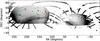 |
Fig. 1 Equatorial map showing the position of all the fields used in this work. The different colours and symbols indicate how the fields have been grouped to calculate the different density profiles. The background image is the SDSS-DR8 map from Koposov et al. (2012), which shows the footprint of the Sagittarius stream and the location of the Sagittarius dwarf galaxy. When grouping the fields, we have also taken into account the presence of this stream, the Triangulum-Andromeda overdensity, and the anticentre substructures (ACS, EBS, and Monoceros), in trying to combine their effect in certain profiles and avoid it in others. |
Our pointings are distributed over the region of the sky visible to both the CFHT and the INT (see Fig. 1). To optimize the star-galaxy separation (see Sect. 2.2) we restrict our analysis to exposures with image quality of subarcsecond seeing, typically < ≈ 0.9 arcsec in the r band. This limitation, combined with the varying fields of view and observing conditions between the data sets, leads to pointing footprint sizes that range between 0.24 and 1.14 deg2.
2.2. Image correction of the PSF distortion (and implications for the star-galaxy separation)
Previous research by our group has shown that the performance of standard star-galaxy separation methods based on the size and ellipticity of the sources can be improved by homogenizing the point-spread function (PSF) across an image prior to its photometric analysis (Pila-Díez et al. 2014). In addition, such a correction also provides the benefit of allowing us to perform fixed aperture photometry and colour measurements.
In order to homogenize the PSF of our images, we use a code (Pila-Díez et al. 2014) that, as a first step, takes the shape of the bright stars in a given image and uses it to map the varying PSF and, as a second step, convolves this map with a spatially variable kernel designed to transform everywhere the original PSF into a Gaussian PSF.
2.3. Catalogues
From the PSF-homogenized exposures we create photometric catalogues using Source Extractor (Bertin & Arnouts 1996). For the g and the r data, we stack the different exposures in each band to create a single calibrated image, and we extract the band catalogues from them. We perform a star-galaxy separation based on the brightness, size and ellipticity of the sources and we match the surviving sources in the two catalogues to produce a gr-catalogue of stars for each field of view (see Pila-Díez et al. 2014). The limiting magnitudes of these gr star catalogues reach mAB ~ 25.0 at the 5.0σ level in the r band.
For the U and the i fields of view, we produce several photometric catalogues, one for each individual exposure. We correct the magnitudes in the i catalogues for the dependency of the illumination on pixel position. For each pointing and band, the exposure catalogues are calibrated to a common zero point and combined to produce a single-band catalogue. In these single-band catalogues, the resulting magnitude for each source is calculated as the median of the contributions of all the individual exposures. At this point the U and the i magnitudes are converted from the INT to the CFHT photometric system using the following equations, which we derive by calibrating our mixed INT-CFHT colours to the colour stellar loci of the CFHT Legacy Survey (Erben et al. 2009; Hildebrandt et al. 2009):  Finally we position-match the sources from the U-, the i- and the gr-catalogues to create a final catalogue of stellar sources for each field of view. These final ugri-catalogues are shallower than the gr-catalogues because of the lesser depth of the i and the U observations (see Table 1). Figure 2 shows the colour-magnitude diagrams (CMDs) for the final ugri and gr catalogues (top and centre, respectively), and the difference between them (bottom). The bottom panel highlights that, in the colour regime of the halo (0.2 <g − r< 0.3), the combination of the four bands removes mainly very faint, unresolved galaxies.
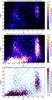 |
Fig. 2 Hess diagrams showing the number of sources per colour−magnitude bin in the ugri catalogue (top), in the gr catalogue (centre) and the difference between both (bottom) for field A1033. Most of the sources lost when combining the catalogues correspond to faint magnitudes, because the i and the U observations are shallower. The effect is the removal of most of the faint galaxies (located in the −0.2 <g − r< 0.7 and r> 23 region in the central panel), most of the faintest disk M dwarves (1.1 <g − r< 1.3) and a number of faint objects (in the i or the U bands) scattered throughout the (g − r,r) diagram. |
We correct for interstellar extinction using the maps from Schlegel et al. (1998) and transform the magnitudes in the ugri-stellar catalogues from the CFHT to the SDSS photometric system. For this we use the equations on the Canadian Astronomy Data Center MegaCam website1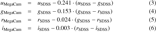 and invert them to turn our measurements into SDSS magnitudes. Subsequently we calibrate each field directly to SDSS using stellar photometry from DR8. The resulting photometry matches the colour−colour stellar loci of Covey et al. (2007) as shown in Fig. 3. Unless explicitly stated otherwise, all magnitudes in this paper are expressed in the SDSS system.
In order to reduce the noise when analysing the radial stellar density distribution of the halo, we combine the catalogues from nearby pointings, grouping them according to their position in the sky. This step is important because of the nature of our survey, which is composed of relatively small, scattered fields of view. We use a friends-of-friends (FoF) algorithm to group the different pointings. We request two friends not to be apart by more than 20 deg, and in a few cases we clean or split a resulting group (red pentagons or blue and orange triangles in Fig. 1) or combine others (purple diamonds) to account for the positions of the galactic disk or major halo substructures. Because the different pointings in our surveys have different completeness limits, these grouped or combined catalogues – which we name A,B,C,... H – are finally filtered to meet the completeness magnitude threshold of their most restrictive contributor2.
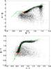 |
Fig. 3 Colour–colour diagrams (CCDs) corresponding to the fields in group A (pointings marked as light cyan circles in Fig. 1). The sources in the ugri catalogues (black) and the subset of near-MSTO stars (red) have been calibrated to SDSS using DR8 stellar photometry. The main sequence stellar loci (green dashed lines) are the ones given in Tables 3 and 4 of Covey et al. (2007). Quasars and white dwarf-M dwarf pairs are abundant in the u − g< 1, −0.3 <g − r< 0.7 space. |
3. Stellar radial density profiles
3.1. Star selection and construction of the radial stellar density profiles
The coordinates and the completeness limits of the groups are given in Table 1. We use halo main sequence turnoff stars in our fields as tracer of the stellar halo: at the completeness limits of the data such stars can be identified as far out as 60 kpc from the Galactic centre. We fit several Galactic stellar distribution models to these density profiles and derive a number of structural parameters for the stellar halo. Previous works have already used main sequence turnoff point (MSTO) stars, near-MSTO stars, BHB and blue stragglers of type A and RR Lyrae as stellar tracers for the Galactic stellar halo. We compare and discuss our findings to theirs in Sect. 4.2.
In order to select the near main sequence turnoff stars we make use of two empirical photometric variables. The ratio [Fe/H] is calculated following the photometric metallicity relation by Bond et al. (2010), and the absolute magnitude Mr is calculated following the photometric parallax relation from Ivezić et al. (2008): ![\begin{eqnarray} [{\rm Fe/H}] &=& -13.13 + 14.09x + 28.04y - 5.51xy -5.90x^2 \nonumber \\ &&\quad - 58.68y^2 + 9.14x^2y - 20.61xy^2 + 58.20y^3, \end{eqnarray}](/articles/aa/full_html/2015/07/aa25457-14/aa25457-14-eq39.png) (7)where x = u − g and y = g − r. This relation is valid in the g − i< 0.6 and −2.5 ≤ [Fe/H] ≤ 0 range, which is compatible with the regime of our near-MSTO star selection.
(7)where x = u − g and y = g − r. This relation is valid in the g − i< 0.6 and −2.5 ≤ [Fe/H] ≤ 0 range, which is compatible with the regime of our near-MSTO star selection. ![\begin{eqnarray} M_r &=& -0.56 + 14.32z - 12.97z^2 + 6.127z^3 -1.267z^4 \nonumber\\ &&\quad + 0.0967z^5 -1.11[{\rm Fe/H}] - 0.18[{\rm Fe/H}]^2, \end{eqnarray}](/articles/aa/full_html/2015/07/aa25457-14/aa25457-14-eq44.png) (8)where z = g − i. The tested validity regime of this equation encompasses the 0.2 <g − i< 1.0 range, meaning that the absolute brightnesses of our near-MSTO stars have been properly estimated. We extrapolate the relation for the 0.1 <g − i< 0.2 range, which is justified owing to the smooth and slow change of Mr with z.
(8)where z = g − i. The tested validity regime of this equation encompasses the 0.2 <g − i< 1.0 range, meaning that the absolute brightnesses of our near-MSTO stars have been properly estimated. We extrapolate the relation for the 0.1 <g − i< 0.2 range, which is justified owing to the smooth and slow change of Mr with z.
We select the halo near-MSTO stars by requiring ![\begin{eqnarray} & &0.2 < g-r < 0.3 ; \label{constr:g-r} \\ & &g,r,i > 17 ; \label{constr:gri} \\ &&0.1 < g-i < 0.6 ; \label{constr:g-i} \\ &&5.0 > M_r > -2 ; \label{constr:absMag} \\ && - 2.5 \leq [{\rm Fe/H}] \leq 0 \label{constr:metal} . \end{eqnarray}](/articles/aa/full_html/2015/07/aa25457-14/aa25457-14-eq49.png) The first two restrictions (9 and 10) retrieve stars typically associated with the halo, in particular distant main sequence F stars (see Table 3 from Covey et al. 2007). This selection however, can be significantly contaminated by quasars and white dwarf-M dwarf pairs, which are abundant in (but not restricted to) the −0.2 <g − r< 0.3 range (see Fig. 3). To reduce the presence of these interlopers and select the bulk of the F stars population, we apply restrictions 11 (based on Table 4 in Covey et al. 2007) and 12. Constraint 13 ensures that the final sources are at most as metal rich as the Sun (to account for possible contributions from metal-rich satellites) and not more metal-poor than 0.003 times the Sun.
The first two restrictions (9 and 10) retrieve stars typically associated with the halo, in particular distant main sequence F stars (see Table 3 from Covey et al. 2007). This selection however, can be significantly contaminated by quasars and white dwarf-M dwarf pairs, which are abundant in (but not restricted to) the −0.2 <g − r< 0.3 range (see Fig. 3). To reduce the presence of these interlopers and select the bulk of the F stars population, we apply restrictions 11 (based on Table 4 in Covey et al. 2007) and 12. Constraint 13 ensures that the final sources are at most as metal rich as the Sun (to account for possible contributions from metal-rich satellites) and not more metal-poor than 0.003 times the Sun.
The decrease in interlopers attained by applying restrictions 11, 12, and 13 compared to only applying restrictions 9 and 10 is illustrated in Fig. 3, where the red dots indicate the final selection of halo near-MSTO stars and the black dots represent the whole catalogue of star-like sources. It is clear that the final selection of near-MSTO stars does not span the whole range of sources encompassed between g − r = 0.2 and g − r = 0.3. The effect of the [Fe/H] and Mr selection is further illustrated in Fig. 4.
Using the estimated absolute brightness, we calculate the distance modulus and the heliocentric distance for all the near-MSTO stars. We define distance modulus bins of size Δμ = 0.2 mag and Δμ = 0.4 mag, and count the number of near-MSTO stars per bin for each group of fields (A, B, C,...). The choice of distance bins is motivated by a compromise between maximising the radial distance resolution and minimising the Poisson noise in the stellar number counts. We test this compromise by exploring two distance modulus bin sizes, which correspond to distance bin sizes of the order of 102 pc and 10 kpc, respectively.
We then calculate the number density per bin and its uncertainty as follows:  where ΔΩ is the area covered by each group, DhC is the heliocentric distance, l and b are the galactic coordinates and Nl,b,Δμ is the number of stars per bin in a given direction of the sky. Particularly,
 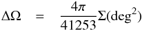 (16)and the area of each group (Σ) depends on the individual area of each field contributing to it (Table 1).
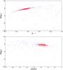 |
Fig. 4 Estimated absolute magnitude in the r band (Mr) and estimated metallicity ([Fe/H]) for group A for the sources typically considered as halo stars (blue) and those that we have selected as near-MSTO stars (red). The sources selected as halo members meet 0.2 <g − r< 0.3 and g,r,i> 17. The subset of near-MSTO stars, additionally meets Mr> − 2, −2.5 ≤ [Fe/H] ≤ 0 and 0.1 <g − i< 0.6. |
The results for these number density calculations can be seen in Fig. 5, where we plot the logarithmic number density against the galactocentric distance3, RGC, for each group (or line of sight). For this and the subsequent analysis, we only consider bins with RGC> 5 kpc, | z | > 10 kpc (to avoid the inner regions of the Galaxy) and a distance modulus of μ ≤ maglim − 4.5 (to guarantee a complete sample of the faintest near-MSTO stars4).
Figure 5 shows that the density profiles decrease quite smoothly for 40 − 60 kiloparsecs and for most of the lines of sight.
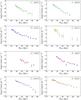 |
Fig. 5 Logarithmic stellar density profiles versus distance for the near Main Sequence turnoff point stars (near-MSTO) from the fields in groups A (green circles), B (cyan squares), C (blue downward triangles), D (yellow upward triangles), E (red pentagons), F (pink hexagons), G (purple diamonds) and H (orange leftward triangles). Their symbols match those in Fig. 1. |
3.2. Fitting procedure
We fit several models of the Galactic stellar number density distribution to the data, ranging from a basic axisymmetric power law to more complex models with triaxiality and a break in the power law. The models take the following mathematical forms, with x, y, and z being the cartesian galactocentric coordinates with the Sun at (8, 0, 0) kpc (Malkin 2012):
-
Axisymmetric model
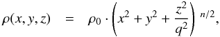 (17)where q = c/a is the polar axis ratio or the oblateness of the halo;
 -
Triaxial model
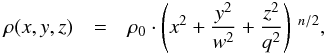 (18)where w = b/a is the ratio between the axes in the Galactic plane;
 -
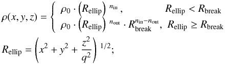
Broken power law, with varying power index and oblateness at Rbreak
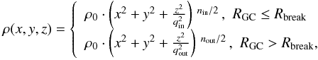 (20)where the inner power law is fit to data that meets RGC ≤ Rbreak and the outer power law is applied to data that meets RGC>Rbreak.
We fit all these models to the data using the “curve-fit” method from Scipy.optimize, which uses the Levenberg-Marquardt algorithm for non-linear least squares fitting. The objective function takes the form of a χ2, and we also calculate a reduced χ2 for analysis purposes,  where Ndata and Nparams are the number of data points and the number of free parameters, respectively.
The influence of the photometric uncertainties on the density profiles and the best fit parameters is evaluated through a set of Monte Carlo simulations that randomly modify the g,r,i,u magnitudes of each star within the limits of the photometric uncertainties. Through this method we find that the variation of the Monte Carlo best fit parameters aligns with the uncertainties of our best fit parameters (derived from the second derivative of the fits by the “curve-fit” method). The centre of these variations is within 1σ of our direct findings.
We fit all models to four data sets: with and without (known) substructures and binned in 0.2 and 0.4 mag cells. In this way we can check the robustness of our results to different binning options and we are able to compare what would be the effect of substructure on our understanding of the smooth halo if we were to ignore it or unable to recognize it as such. Specifically, we cut the distance bins at RGC< 25 kpc in group E to avoid contributions by the structures in the direction of the galactic anticentre (the Monoceros ring, the Anticentre Structure and the Eastern Band Structure), the distance bins within 15 <DhC< 40 kpc in group G to avoid contributions by the Sagittarius stream, and the distance bins within 20 kpc <DhC< 60 kpc in group H to avoid contributions again by the Sagittarius stream.
3.3. Results
The best fit parameters for each model resulting from fitting these four data sets are summarized in Tables 2 to 5. Table 2 contains the results of fitting the Δμ = 0.2 mag binned data excluding regions with substructure, whereas Table 3 contains the results of fitting to all the 0.2 mag bins. Similarly Table 4 covers the fits to Δμ = 0.4 mag data without substructure bins, and Table 5, to all 0.4 mag bins. The reduced χ2 and the initial parameters have also been recorded in these tables.
Best fit parameters for the four different Galactic stellar distribution models resulting from removing the data that is affected by known halo substructures (the Sagittarius stream and the anticentre substructures).
We compare the fitting results for the four different data sets recorded in Tables 2 to 5 and find that the fits for which the substructure has been masked significantly outperform those that have been allowed to fit all the available data. The difference on  for all these models and bin sizes is in every case at least a factor of 2.3 or larger. We find that allowing the models to fit data that contains substructure does not affect largely most of the structural parameters (polar axis ratios are compatible within the uncertainties and power law indices have close values) except that it decreases the disk axis ratio w by at least 10%, suggesting a strong departure from the axisymmetric model that is not implicit in the filtered data sets. Henceforth we will restrict the remaining discussion to the results derived from the cleanest data sets.
Comparing the parameters resulting from the best fits to the masked 0.2 mag and 0.4 mag data, we find that the fits to 0.2 mag binned data perform better for all the models ( ratio of two). Nonetheless, all the measurements for the different structural parameters in the two data sets are compatible with each other within the uncertainties. The best fits for the four models and their residuals for our eight lines of sight are shown in Figs. 6a and b for the masked 0.2 mag binned data. It is clear that the differences between the fitted models along these sight lines are small.
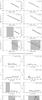 |
Fig. 6 Left panels: density profiles in decimal logarithmic scale and the best fit models from Table 2 (fitted to masked 0.2 binned data). Right panels: residuals between the data and the best fit models from panel 6a. The different lines represent the axisymmetric (black solid line), the triaxial (green dashed line), the broken power law with varying power index (red dotted line) and the broken power law with varying power index and oblateness (blue dashed-dotted-dotted line) models. The grey areas denote data that have been masked from the fitting to account for the presence of substructure. |
Our data are inconclusive regarding triaxiality, but are compatible with either a mildly triaxial halo or with no triaxiality. For the 0.2 mag data set, the triaxial model fits slightly better than the axisymmetric model and returns w = 0.87 ± 0.09. For the 0.4 mag data set, however, the axisymmetric model fits slightly better and the triaxial model returns a disk axis ratio compatible with 1. In both data sets the other best-fitting parameters are practically identical for the two models. This indicates that the cost of the extra parameter is not supported by the 0.4 mag data. Thus, it is hard to derive a precise value for the disk axis ratio and to conclude if it is truly triaxial, but a weighted average of w and the general analysis show confidently that w> 0.8.
We increase the complexity of the axisymmetric model by adding two degrees of freedom and considering a change in the power law index n at a specific break distance Rbreak (a broken power law). For this purpose, we use a grid of values to explore all the parameters except the density scale factor ρ0, which we left free to fit (see below for the grid characterization). This model decreases the in both the 0.2 and the 0.4 mag binned cases, indicating that our data is better fit by a broken power law than by a simple axisymmetric model or a triaxial model. It turns the single power law index from n = −4.26 ± 0.06 into a less steep inner index nin = −2.50 ± 0.04 and a steeper outer index nout = −4.85 ± 0.04 (measurements here are for weighted averages between the 0.2 and 0.4 mag data). It also increases the central value of the polar axis ratio q within the uncertainties, from a weighted q = 0.77 ± 0.04 to a weighted q = 0.79 ± 0.02. Globally, the disk axis ratio seems to be the most stable parameter throughout the different model fits to our data, returning a moderately oblate halo.
Finally we fix the break distance at the best fit value found by the broken power law model (Rbreak = 19 kpc and 20 kpc for the 0.2 and 0.4 mag binned data, respectively) and add another parameter to it, allowing not only n, but also q to change at the break distance. We find that the best fits to this model return such large error bars for the inner halo that, in practice, it yields unconstrained measurements: Δρ0 ≤ ρ0, Δnin is 12−18% of nin and Δqin is 30% of qin.
We explore each model to investigate possible parameter degeneracies, tolerance ranges and potential local minima in our best fits. For this we fix all the parameters in the four models except the density scale factor ρ0, and we run the fits across a grid of parameter values. In particular, the grids are built following q2,w2 ∈ [0.1,2.0;δ = 0.05], n ∈ [−5.0 −1.0;δ = 0.1], nin ∈ [−4.0, −1.0;δ = 0.1], nout ∈ [−7.0, −3.0;δ = 0.2] and Rbr ∈ [15,50;δ = 1], where δ is the incremental step for each parameter. We find that there is a degeneracy between Rbr and nin for the simple broken power law model for both binnings (see Fig. 7).
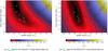 |
Fig. 7
|


Finally our measurements for the density scale factor ρ0 (ρ at RGC = 1 kpc) are the result of large extrapolations and merely serve as normalizations for our fits. For that reason we do not discuss these values in detail.
4. Discussion
4.1. Robustness of the best fit structural parameters
In order to determine how the data available to us influences the results from our best fits, we remove the different lines of sight one at a time and repeat the fits. In this way we can determine which are the most critical lines of sight and what is their effect on our results.
We find that most of them have no significant influence on the best fit parameters of the different halo models. However, starting with the polar axis ratio we find that removing group A increases slightly its value (q ≈ 0.85) and removing groups C or E decreases it slightly (q ≈ 0.70) in both the axisymmetric and triaxial model in the two data sets. Regarding the power law index, again groups A or C have an influence, but group B as well. Removing groups A or B increases n to ≈ − 4.1 ± 0.1, whereas removing C decreases it to n ≈ − 4.6. When considering a triaxial halo, we find that groups A, B or C increase the disk axis ratio w by ~0.10, and that removing groups E or F decreases it to w ≈ 0.7. Additionally, in conditions of triaxiality, the lack of group E reduces q further to q ≈ 0.60.
Thus removing group E turns out to be critical for both q and w, representing a rather differently looking halo (significantly oblate and quite elliptical in the plane). Group F also has a similar effect on w but not on q. The reason why group E has such a strong influence in the determination of a possible triaxiality is that it is by far the closest group to the Galactic anticentre. Other groups also influence the measurements of the different parameters, but have a smaller influence on the general picture we would derive. Overall we see that the lines of sight we use can have a drastic effect on the w results and a significant but moderate effect on q and n. This means that a global view of the halo is essential owing to its complex structure.
4.2. Comparison to previous studies
Previous investigations using near-MSTO stars have explored both the inner and the outer halo out to moderate distances (30 − 40 kpc), and similar regimes have been probed with blue horizontal branch stars and blue struggler stars, MSTO stars or multiple stellar halo tracers. Studies involving RR Lyrae stars have reached further out to 50 kpc. Remarkably, the depth of our data allows us to probe further than any previous study (out to 60 kpc) in several directions, independently of the stellar tracer.
In this section we compare our findings regarding the structural parameters of the stellar halo to those of the following results in the literature:
-
Jurić et al. (2008)use near-MSTO stars from the SDSS-DR3and DR4 as stellar tracers, and cover the5 kpc < RGC < 15 kpc range. They comprise 5450 deg2 in the northern Galactic hemisphere and 1088 deg2 in the south.
-
Sesar et al. (2011) use as well near-MSTO stars from the CFHT Legacy Survey, and explore the 5 kpc < RGC < 35 kpc range. Two of their four fields explore the South Galactic Cap.
-
Deason et al. (2011) use type A blue horizontal branch (BHB) stars and blue stragglers (BS), reaching out to RGC = 40 kpc.
-
de Jong et al. (2010) use CMD fitting of SEGUE stellar photometry to probe the total stellar mass density from RGC = 7 kpc to RGC = 30 kpc along a “picket fence” of 2.5 deg wide strips at fixed Galactic longitude spanning a large range of Galactic latitudes.
-
Chen et al. (2001) use more general MSTO stars from two high latitude regions of SDSS to the North and the South of the Galactic plane (49 deg < |b| < 64 deg). They explore the inner halo regime (RGC ≲ 30 kpc).
-
Bell et al. (2008) use also more general MSTO stars from SDSS-DR5 spanning 5 < RGC < 40 kpc.
-
Faccioli et al. (2014) use RR Lyrae in the 9 kpc < RGC < 49 kpc range. Their multiepoch data comes from the Xuyi Schmidt Telescope Photometric Survey (XSTPS) in combination with SDSS colours, and covers 376.75 deg2 at RA ≈ 150 deg and Dec ≈ 27 deg.
-
Sesar et al. (2010) use RR Lyrae stars from SDSS-II in the stripe 82 region. Although their data originally spans 5 kpc < RGC < 110 kpc, the reanalysis performed by Faccioli et al. (2014) to derive structural parameters truncates the sample at 49 kpc.
-
Watkins et al. (2009) use as well RR Lyrae from SDSS in stripe 82, and the comparative derivation of structural parameters by Faccioli et al. (2014) also truncates it at 49 kpc. Stripe 82 is located in the South Galactic Cap.
The result of this comparison is summarized in Table 6. We note that the oblateness values for Faccioli et al. (2014), Sesar et al. (2010) and Watkins et al. (2009) are not the result of absolute best fits to a set of free parameters, but the best fits to free Rbr, nin and nout with fixed prior values for a quite oblate ( ) and a moderately oblate halo (q = 0.70 ± 0.01).
All surveys that reach beyond RGC = 30 kpc coincide in the need for a break in the power-law index of the halo density. Regarding possible triaxiality, only a few of the studies report constraints on w. Those that do, have either reported “finding unreasonable values” (Sesar et al. 2011) or have obtained limits on triaxiality similar to ours (w > 0.8, Bell et al. 2008).
On the break radius, there is a general consensus towards Rbreak ≈ 27 kpc. The only exception is that of Bell et al. (2008), who find a value very close to our measurement (~20 kpc). These discrepancies, however, can be explained by the effect of the Rbreak − nin degeneracy discussed in Sect. 3.3.
The inner and outer halo power law indices mostly fall in the [− 2.3, − 3.0] and [−3.6, −5.1] ranges. Our inner power law index nin = −2.50 ± 0.04 is consistent with these results, particularly with the lower end. In the case of the outer halo power index (nout = −4.85 ± 0.04), the comparison is less trivial. First, only Sesar et al. (2011) and Deason et al. (2011) have provided measurements for nout based on fits with a free q parameter (nout = −3.8 ± 0.1 and  , respectively). Second, only one work with nout measurements (Sesar et al. 2011) uses a stellar tracer similar to ours (the others use A-BHB and BS stars, or RR Lyrae stars). Most important, a good constraint on nout requires deep data, and none of these earlier surveys reach as deep as our data set. Our steep outer index, although well in the range of previous measurements, might well indicate a progressive steepening of the halo density, though it would be good to test this with additional sight lines of comparable depth. In any case, it seems safe to conclude that nout < −4.0.
The best fit values for the polar axis ratio or oblateness q range from 0.5 to 0.9, with most of the measurements concentrated within (0.55,0.70). The values of q do not seem to depend on whether a break was detected or not, nor on the limiting distance of the survey or on the stellar tracer. The discrepancies can thus be attributed either to methodological differences or to differences in the spatial coverage of the data samples. However, it is difficult to determine the actual cause. Our results do not fit well within the most constricted range but rather within the upper part of the broader range.
Finally it is noteworthy that the choice of stellar tracer across the different works does not seem to cause any significant bias on the best fit parameters.
Comparison between the best fit structural parameters found in this work (weighted averages for the parameters of the 0.2 and 0.4 mag data sets) and those reported by other groups in previous works.
4.3. Detection of overdensities and identification
We analyse the data-to-models residuals for the different lines of sight in Fig. 6b in search for overdensities. We find that, in general, all the lines of sight present regions with data-to-models deviations of a maximum factor of two. Additionally, certain lines of sight – C, D, G, and H – present more significant deviations spanning from a few kiloparsecs to tens of kiloparsecs in distance. We discuss these overdensities in greater detail below, and we also discuss expected overdensities that show no signature in our data.
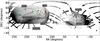 |
Fig. 8 Equatorial map showing the position of all the fields used in this work and the closest cold stellar overdensities to them. These overdensities are used for comparison and discussion of the stellar density profile data-to-model residuals throughout Sect. 4.3. The labels in the figure correspond to the Anticentre Structure (ACS), the Eastern Band Structure (EBS), the NGC 5466 stream, the Grillmair & Dionatos stream (G&D), the Orphan stream, the Triangulum-Andromeda overdensity (Tri-And) and the Pisces overdensity. The background image is the SDSS-DR8 map from Koposov et al. (2012), which shows the footprint of the Sagittarius stream. The Monoceros ring also appears partially in this background image, as a dark region overlapping the western part of the Galactic disk in the anticentre region, eastwards of the ACS. |
The most prominent overdensities in the data-to-model residuals correspond to the northern wrap of the Sagittarius (Sgr) stream. This stream overlaps in projection with groups G and H (see Fig. 8). For group G, the residuals indicate overdensities in the distance range where we expect to find both the Sgr and the Orphan stream (20 <DhC ≲ 40 kpc or 25 <DGC ≲ 44 kpc, Pila-Díez et al. 2014). The overdensities indeed peak between RGC = 25 kpc and 45 kpc, reaching ρ/ρM = 7 ± 2, and drop sharply afterwards. Group H probes the Sgr stream closer to the Galactic centre but also for larger distances than group G. Based both on extensive data (summarized in Pila-Díez et al. 2014) and in models (Law & Majewski 2010 and Peñarrubia et al. 2010), we expect this stream to span the 20 <DhC< 60 kpc or 16 <RGC< 55 kpc range at these coordinates. This expectation is met all along: they steadily increase from RGC ≈ 15 kpc, depart from ρ/ρM = 3 ± 1 at RGC = 30 kpc, reach ρ/ρM = 6 ± 2 at RGC = 40 kpc and peak at RGC = 45 kpc with max(ρ/ρM) = (12,15) ± 2. However, they do not decrease near RGC = 55 kpc but seem to stay stable with a significant ρ/ρM> 7 ± 2. This suggests a thicker branch than predicted by the models, but in agreement with previous RR Lyrae measurements (Ibata et al. 2001; Totten & Irwin 1998; and Dohm-Palmer et al. 2001, as summarized in Fig. 17 of Majewski et al. 2003).
Two more modest overdensities that do not appear in the literature seem to be present in groups C and D. In group C, a weak but consistent overdensity spans a distance range of RGC ≈ 35 kpc to RGC ≈ 60 kpc. In group D, a sharp bump extends over a few kiloparsecs around RGC ≤ 20 kpc.
We have looked for other known overdensities that position-match our lines of sight (see Fig. 8), but found no indication of them in the residuals. The first one corresponds to the tidal tails of the NGC 5466 globular cluster (Belokurov et al. 2006a), which overlap with one field in group A and another one in group B (A1361 centred at (RA,Dec) = (176.09,46.39) and A1927 at (RA,Dec) = (217.92,25.67)). This is a very weak cold substructure located at RGC ≈ = 16 kpc and extending for 45deg with an average width of 1.4deg (Grillmair & Johnson 2006). As such, it is not surprising to find no signature in the density profiles.
The second one is the ensemble of three known overdensities in the direction of group E: the Anti Center Stream (RGC = 18 ± 2 kpc, Rocha-Pinto et al. 2003; Li et al. 2012), the Monoceros ring (RGC ≈ 18 kpc, Li et al. 2012) and the Eastern Band Structure (RGC = 20 ± 2 kpc, Li et al. 2012). These substructures are masked from our fits and residuals when we impose |z| > 10 kpc to avoid the influence of the thick disk, and therefore, they cannot be detected.
The Triangulum-Andromeda overdensity (Martin et al. 2007) falls close to one of the fields in group F. Despite this proximity, the residuals show no evidence for an overdensity at the expected distance of RGC ≈ 30 kpc, indicating that the overdensity does not extend further in this direction.
5. Conclusions
In this paper we have used wide-field images from the CFHT and the INT telescopes in eight broad lines of sight spread across the sky to produce deep photometric catalogues of halo near main sequence turnoff (near-MSTO) stars. Our images have been corrected for PSF inhomogeneities, resulting in catalogues with fixed-aperture colour measurements and improved star-galaxy separation. Thanks to the depth and quality of our data, we reach stellar completeness limits ranging from 22.7 mag to 24.2 mag in the r band, which translate into a 60 kpc distance limit for near-MSTO stars.
We calculate galactocentric distances for the stars based on the photometric parallax method by Ivezić et al. (2008) and the metallicity estimator by Bond et al. (2010). We bin them by distance modulus, and calculate the stellar number density distribution along the eight different lines of sight.
In selecting the halo near-MSTO stars, we have used additional constraints than the standard 0.2 <g − r< 0.3 and g,r,i> 17 cuts in order to obtain a cleaner sample. Particularly, by applying additional cuts based on g − i colour, absolute magnitude and metallicity, we get a sample of mainly F stars significantly decontaminated from quasars and white dwarf-M dwarf pairs.
We fit several galactic halo models of the stellar distribution to our eight lines of sight, and explore the structural parameters resulting from the best fits, as well as the influence of substructure in those parameters. We find that the halo is best represented by a broken power law with index nin = −2.50 ± 0.04 in the inner halo (R<Rbreak = 19.5 ± 0.04) and nout = −4.85 ± 0.04 in the outer halo. Our data cannot constrain whether a change in the polar axis ratio also accompanies the break in the halo. The best fit values for the polar axes ratio indicate a moderately oblate halo: q = 0.79 ± 0.02. The simpler (non-broken) triaxial power law models favour a practically axisymmetric halo, with w ≥ 0.88 ± 0.07 and the rest of parameters equal to those of the axisymmetric one.
We find that fitting models to data that contains substantial substructure can bias significantly the perception of triaxiality, decreasing the disk axis ratio w by 10%. We also find that different distance modulus bin sizes and the inclusion or exclusion of particular lines of sight can moderately influence our measurements of some structural parameters. This calls for carefully crafted analysis and tailored tests in any future studies. When compared to previous works, the choice of stellar tracer seems to have no significant influence on the values of the structural parameters, at least for these distance ranges.
Comparing our density profiles to the smooth model fits, we recover the presence of the Sagittarius stream in groups G and H. The Sagittarius stream in the direction of group H seems to extend further out from the Galactic centre than the models have so far predicted, and confirms previous RR Lyrae detections associated with the stream at such distances (Ibata et al. 2001; Totten & Irwin 1998; Dohm-Palmer et al. 2001). We also find evidence of more modest substructures extending over a long range of distances in group C (35 ≤ RGC ≤ 60 kpc) and quite concentrated in distance in group D (RGC ≈ 20 kpc).
Our pencil beam survey has demonstrated that even a relatively small numbers of narrow fields of view, provided they are sampled sufficiently deep and with an abundant tracer, can place competitive limits on the global density profile and shape of the Galactic halo. The advent of similarly deep, wide-area surveys – like KiDS, VIKING and LSST – therefore promises to enhance substantially our understanding of the halo.
To determine the completeness limit of each field of view, we fit its magnitude distribution to a Gaussian – representing the population of faint galaxies – and another variable function – representing the stellar distribution along the whole magnitude range. We choose as the completeness limit either the transition point between the two distributions (the valley) or, if instead there is a plateau, the turning point of the whole distribution (the knee).

This constraint guarantees that there are no distance completeness issues due to our specific type of stellar tracers and due to the different depths of our fields. The only subset affected by incompleteness is that of maglim − 5.0 <μ< maglim − 4.5 for the stars in the 4.5 <Mr< 5.0 range; and its average loss is of 20% over the total number of near-MSTO stars (−2.0 <Mr< 5.0) in the same distance range. Several tests on different upper distance thresholds for the density profiles show that the distance modulus constraint of μ ≤ maglim − 4.5 is enough to guarantee that all the lines of sight contribute robust density measurements at the furthest distances and that the incompleteness in maglim − 5.0 <μ< maglim − 4.5 for the 4.5 <Mr< 5.0 near-MSTO stars has no statistically significant effect on the best fit parameters.
Acknowledgments
This work is based on observations made with the Isaac Newton Telescope through program IDs I10AN006, I10AP005, I10BN003, I10BP005, I11AN009, I11AP013. The Isaac Newton Telescope is operated on the island of La Palma by the Isaac Newton Group in the Spanish Observatorio del Roque de los Muchachos of the Instituto de Astrofísica de Canarias. It is also based on observations obtained with MegaPrime/MegaCam, a joint project of CFHT and CEA/IRFU, at the Canada-France-Hawaii Telescope (CFHT). The CFHT is operated by the National Research Council (NRC) of Canada, the Institut National des Science de l’Univers of the Centre National de la Recherche Scientifique (CNRS) of France, and the University of Hawaii. Most of the data processing and analysis in this work has been carried out using Python and, in particular, the open source modules Scipy, Numpy, AstroAsciiData and Matplotlib. We have also used the Stilts program for table manipulation. We acknowledge the anonymous referee for the constructive suggestions and insightful discussion. B.P.D. is supported by NOVA, the Dutch Research School of Astronomy. H.H. and R.vdB. acknowledge support from the Netherlands Organisation for Scientific Research (NWO) grant number 639.042.814. We thank Malin Velander, Emma Grocutt, Lars Koens, David Harvey and Catherine Heymans for help in acquiring the INT data.
References
- Ahn, C. P., Alexandroff, R., Allen de Prieto, C., et al. 2014, ApJS, 211, 17 [NASA ADS] [CrossRef] [Google Scholar]
- Bell, E. F., Zucker, D. B., Belokurov, V., et al. 2008, ApJ, 680, 295 [NASA ADS] [CrossRef] [Google Scholar]
- Belokurov, V., Evans, N. W., Irwin, M. J., Hewett, P. C., & Wilkinson, M. I. 2006a, ApJ, 637, L29 [NASA ADS] [CrossRef] [Google Scholar]
- Belokurov, V., Zucker, D. B., Evans, N. W., et al. 2006b, ApJ, 642, L137 [NASA ADS] [CrossRef] [Google Scholar]
- Belokurov, V., Evans, N. W., Irwin, M. J., et al. 2007, ApJ, 658, 337 [Google Scholar]
- Bertin, E., & Arnouts, S. 1996, A&AS, 117, 393 [NASA ADS] [CrossRef] [EDP Sciences] [Google Scholar]
- Bildfell, C., Hoekstra, H., Babul, A., et al. 2012, MNRAS, 425, 204 [NASA ADS] [CrossRef] [Google Scholar]
- Bond, N. A., Ivezić, Ž., Sesar, B., et al. 2010, ApJ, 716, 1 [NASA ADS] [CrossRef] [Google Scholar]
- Chen, B., Stoughton, C., Smith, J. A., et al. 2001, ApJ, 553, 184 [NASA ADS] [CrossRef] [Google Scholar]
- Covey, K. R., Ivezić, Ž., Schlegel, D., et al. 2007, AJ, 134, 2398 [NASA ADS] [CrossRef] [Google Scholar]
- de Jong, J. T. A., Yanny, B., Rix, H.-W., et al. 2010, ApJ, 714, 663 [NASA ADS] [CrossRef] [Google Scholar]
- Deason, A. J., Belokurov, V., & Evans, N. W. 2011, MNRAS, 416, 2903 [NASA ADS] [CrossRef] [Google Scholar]
- Dohm-Palmer, R. C., Helmi, A., Morrison, H., et al. 2001, ApJ, 555, L37 [NASA ADS] [CrossRef] [Google Scholar]
- Erben, T., Hildebrandt, H., Lerchster, M., et al. 2009, A&A, 493, 1197 [NASA ADS] [CrossRef] [EDP Sciences] [Google Scholar]
- Faccioli, L., Smith, M. C., Yuan, H.-B., et al. 2014, ApJ, 788, 105 [NASA ADS] [CrossRef] [Google Scholar]
- Grillmair, C. J. 2006, ApJ, 651, L29 [NASA ADS] [CrossRef] [Google Scholar]
- Grillmair, C. J., & Johnson, R. 2006, ApJ, 639, L17 [NASA ADS] [CrossRef] [Google Scholar]
- Hildebrandt, H., Pielorz, J., Erben, T., et al. 2009, A&A, 498, 725 [NASA ADS] [CrossRef] [EDP Sciences] [Google Scholar]
- Hoekstra, H., Mahdavi, A., Babul, A., & Bildfell, C. 2012, MNRAS, 427, 1298 [NASA ADS] [CrossRef] [Google Scholar]
- Ibata, R., Lewis, G. F., Irwin, M., Totten, E., & Quinn, T. 2001, ApJ, 551, 294 [NASA ADS] [CrossRef] [Google Scholar]
- Ivezić, Ž., Sesar, B., Jurić, M., et al. 2008, ApJ, 684, 287 [NASA ADS] [CrossRef] [Google Scholar]
- Jurić, M., Ivezić, Ž., Brooks, A., et al. 2008, ApJ, 673, 864 [NASA ADS] [CrossRef] [MathSciNet] [Google Scholar]
- Koposov, S. E., Belokurov, V., Evans, N. W., et al. 2012, ApJ, 750, 80 [NASA ADS] [CrossRef] [Google Scholar]
- Law, D. R., & Majewski, S. R. 2010, ApJ, 714, 229 [NASA ADS] [CrossRef] [Google Scholar]
- Li, J., Newberg, H. J., Carlin, J. L., et al. 2012, ApJ, 757, 151 [NASA ADS] [CrossRef] [Google Scholar]
- Majewski, S. R., Skrutskie, M. F., Weinberg, M. D., & Ostheimer, J. C. 2003, ApJ, 599, 1082 [NASA ADS] [CrossRef] [Google Scholar]
- Malkin, Z. 2012 [arXiv:1202.6128] [Google Scholar]
- Martin, N. F., Ibata, R. A., & Irwin, M. 2007, ApJ, 668, L123 [NASA ADS] [CrossRef] [Google Scholar]
- Newberg, H. J., Yanny, B., Rockosi, C., et al. 2002, ApJ, 569, 245 [NASA ADS] [CrossRef] [Google Scholar]
- Peñarrubia, J., Belokurov, V., Evans, N. W., et al. 2010, MNRAS, 408, L26 [NASA ADS] [Google Scholar]
- Pila-Díez, B., Kuijken, K., de Jong, J. T. A., Hoekstra, H., & van der Burg, R. F. J. 2014, A&A, 564, A18 [NASA ADS] [CrossRef] [EDP Sciences] [Google Scholar]
- Rocha-Pinto, H. J., Majewski, S. R., Skrutskie, M. F., & Crane, J. D. 2003, ApJ, 594, L115 [NASA ADS] [CrossRef] [Google Scholar]
- Sand, D. J., Graham, M. L., Bildfell, C., et al. 2012, ApJ, 746, 163 [NASA ADS] [CrossRef] [Google Scholar]
- Schlegel, D. J., Finkbeiner, D. P., & Davis, M. 1998, ApJ, 500, 525 [NASA ADS] [CrossRef] [Google Scholar]
- Sesar, B., Ivezić, Ž., Grammer, S. H., et al. 2010, ApJ, 708, 717 [NASA ADS] [CrossRef] [Google Scholar]
- Sesar, B., Jurić, M., & Ivezić, Ž. 2011, ApJ, 731, 4 [NASA ADS] [CrossRef] [Google Scholar]
- Skrutskie, M. F., Cutri, R. M., Stiening, R., et al. 2006, AJ, 131, 1163 [NASA ADS] [CrossRef] [Google Scholar]
- Totten, E. J., & Irwin, M. J. 1998, MNRAS, 294, 1 [NASA ADS] [CrossRef] [Google Scholar]
- Watkins, L. L., Evans, N. W., Belokurov, V., et al. 2009, MNRAS, 398, 1757 [NASA ADS] [CrossRef] [Google Scholar]
- York, D. G., Adelman, J., Anderson, J. E., Jr., et al. 2000, AJ, 120, 1579 [Google Scholar]
All Tables
Best fit parameters for the four different Galactic stellar distribution models resulting from removing the data that is affected by known halo substructures (the Sagittarius stream and the anticentre substructures).
Comparison between the best fit structural parameters found in this work (weighted averages for the parameters of the 0.2 and 0.4 mag data sets) and those reported by other groups in previous works.
All Figures
|
Fig. 1 Equatorial map showing the position of all the fields used in this work. The different colours and symbols indicate how the fields have been grouped to calculate the different density profiles. The background image is the SDSS-DR8 map from Koposov et al. (2012), which shows the footprint of the Sagittarius stream and the location of the Sagittarius dwarf galaxy. When grouping the fields, we have also taken into account the presence of this stream, the Triangulum-Andromeda overdensity, and the anticentre substructures (ACS, EBS, and Monoceros), in trying to combine their effect in certain profiles and avoid it in others. |
| In the text | |
|
Fig. 2 Hess diagrams showing the number of sources per colour−magnitude bin in the ugri catalogue (top), in the gr catalogue (centre) and the difference between both (bottom) for field A1033. Most of the sources lost when combining the catalogues correspond to faint magnitudes, because the i and the U observations are shallower. The effect is the removal of most of the faint galaxies (located in the −0.2 <g − r< 0.7 and r> 23 region in the central panel), most of the faintest disk M dwarves (1.1 <g − r< 1.3) and a number of faint objects (in the i or the U bands) scattered throughout the (g − r,r) diagram. |
| In the text | |
|
Fig. 3 Colour–colour diagrams (CCDs) corresponding to the fields in group A (pointings marked as light cyan circles in Fig. 1). The sources in the ugri catalogues (black) and the subset of near-MSTO stars (red) have been calibrated to SDSS using DR8 stellar photometry. The main sequence stellar loci (green dashed lines) are the ones given in Tables 3 and 4 of Covey et al. (2007). Quasars and white dwarf-M dwarf pairs are abundant in the u − g< 1, −0.3 <g − r< 0.7 space. |
| In the text | |
|
Fig. 4 Estimated absolute magnitude in the r band (Mr) and estimated metallicity ([Fe/H]) for group A for the sources typically considered as halo stars (blue) and those that we have selected as near-MSTO stars (red). The sources selected as halo members meet 0.2 <g − r< 0.3 and g,r,i> 17. The subset of near-MSTO stars, additionally meets Mr> − 2, −2.5 ≤ [Fe/H] ≤ 0 and 0.1 <g − i< 0.6. |
| In the text | |
|
Fig. 5 Logarithmic stellar density profiles versus distance for the near Main Sequence turnoff point stars (near-MSTO) from the fields in groups A (green circles), B (cyan squares), C (blue downward triangles), D (yellow upward triangles), E (red pentagons), F (pink hexagons), G (purple diamonds) and H (orange leftward triangles). Their symbols match those in Fig. 1. |
| In the text | |
|
Fig. 6 Left panels: density profiles in decimal logarithmic scale and the best fit models from Table 2 (fitted to masked 0.2 binned data). Right panels: residuals between the data and the best fit models from panel 6a. The different lines represent the axisymmetric (black solid line), the triaxial (green dashed line), the broken power law with varying power index (red dotted line) and the broken power law with varying power index and oblateness (blue dashed-dotted-dotted line) models. The grey areas denote data that have been masked from the fitting to account for the presence of substructure. |
| In the text | |
|
Fig. 7
|
| In the text | |
|
Fig. 8 Equatorial map showing the position of all the fields used in this work and the closest cold stellar overdensities to them. These overdensities are used for comparison and discussion of the stellar density profile data-to-model residuals throughout Sect. 4.3. The labels in the figure correspond to the Anticentre Structure (ACS), the Eastern Band Structure (EBS), the NGC 5466 stream, the Grillmair & Dionatos stream (G&D), the Orphan stream, the Triangulum-Andromeda overdensity (Tri-And) and the Pisces overdensity. The background image is the SDSS-DR8 map from Koposov et al. (2012), which shows the footprint of the Sagittarius stream. The Monoceros ring also appears partially in this background image, as a dark region overlapping the western part of the Galactic disk in the anticentre region, eastwards of the ACS. |
| In the text | |
Current usage metrics show cumulative count of Article Views (full-text article views including HTML views, PDF and ePub downloads, according to the available data) and Abstracts Views on Vision4Press platform.
Data correspond to usage on the plateform after 2015. The current usage metrics is available 48-96 hours after online publication and is updated daily on week days.
Initial download of the metrics may take a while.