| Issue |
A&A
Volume 578, June 2015
|
|
|---|---|---|
| Article Number | A61 | |
| Number of page(s) | 14 | |
| Section | Extragalactic astronomy | |
| DOI | https://doi.org/10.1051/0004-6361/201425267 | |
| Published online | 05 June 2015 | |
Where are compact groups in the local Universe?⋆,⋆⋆
Instituto de Astronomía Teórica y Experimental, IATE, CONICET, Córdoba, Argentina Observatorio Astronómico, Universidad Nacional de Córdoba, Laprida 854, X5000BGR, Córdoba, Argentina
e-mail: This email address is being protected from spambots. You need JavaScript enabled to view it.
Received: 3 November 2014
Accepted: 31 March 2015
Abstract
Aims. The purpose of this work is to perform a statistical analysis of the location of compact groups in the Universe from observational and semi-analytical points of view.
Methods. We used the velocity-filtered compact group sample extracted from the Two Micron All Sky Survey for our analysis. We also used a new sample of galaxy groups identified in the 2M++ galaxy redshift catalogue as tracers of the large-scale structure. We defined a procedure to search in redshift space for compact groups that can be considered embedded in other overdense systems and applied this criterion to several possible combinations of different compact and galaxy group subsamples. We also performed similar analyses for simulated compact and galaxy groups identified in a 2M++ mock galaxy catalogue constructed from the Millennium Run Simulation I plus a semi-analytical model of galaxy formation.
Results. We observed that only ~27% of the compact groups can be considered to be embedded in larger overdense systems, that is, most of the compact groups are more likely to be isolated systems. The embedded compact groups show statistically smaller sizes and brighter surface brightnesses than non-embedded systems. No evidence was found that embedded compact groups are more likely to inhabit galaxy groups with a given virial mass or with a particular dynamical state. We found very similar results when the analysis was performed using mock compact and galaxy groups. Based on the semi-analytical studies, we predict that 70% of the embedded compact groups probably are 3D physically dense systems. Finally, real space information allowed us to reveal the bimodal behaviour of the distribution of 3D minimum distances between compact and galaxy groups.
Conclusions. The location of compact groups should be carefully taken into account when comparing properties of galaxies in environments that are a priori different.
Key words: methods: numerical / methods: statistical / galaxies: groups: general
Appendices are available in electronic form at http://www.aanda.org
Full Tables B.1 and B.2 are only available at the CDS via anonymous ftp to cdsarc.u-strasbg.fr (130.79.128.5) or via http://cdsarc.u-strasbg.fr/viz-bin/qcat?J/A+A/578/A61
© ESO, 2015
1. Introduction
The search for clues that help in unveiling the formation scenario of different structures in the Universe is one of the main goals in current extragalactic astronomy. These clues are searched for everywhere to understand the formation of galaxy systems and the evolution of galaxies in these systems. Studies conducted to improve our understanding of galaxy evolution focus on compact groups because of their extreme nature.
The discovery of compact groups began with Stephan (1877) and Seyfert (1948). Later, the initial discovery of a very compact association of red objects by Shakbazyan in 1957 was confirmed as a galaxy compact group by Robinson & Wampler (1973). This study triggered a systematic search for this type of system. The pioneer works on Shakbazyan compact groups (Shakbazyan 1973; Shakbazyan & Petrosian 1974; Baier et al. 1974; Petrosian 1974, 1978; Baier & Tiersch 1975, 1976a,b, 1978, 1979) were followed by the attempt of Rose (1977) to construct a compact group catalogue, which in turn was followed by the most widely known and most frequently studied Hickson Compact Group catalogue (HCG, Hickson 1982, 1997 and references therein). These small systems of a few galaxies in close proximity have caused the construction of several catalogues of compact groups (e.g. Prandoni et al. 1994; Barton et al. 1996; Focardi & Kelm 2002; Lee et al. 2004; McConnachie et al. 2009; Díaz-Giménez et al. 2012) as well as a host of scientific analyses of their physical properties. Many of these studies have focused on their internal structure by analysing the main characteristics of the galaxy members and aiming to distinguish the nature of compact groups as physical entities (e.g. Mamon 1986; Mendes de Oliveira & Hickson 1991; Moles et al. 1994; del Olmo et al. 1995; Verdes-Montenegro et al. 1994, 2001, 2005; Kelm & Focardi 2004; Martinez et al. 2010; Plauchu-Frayn et al. 2012). Studies were also conducted with the aim of understanding the different formation scenarios that might lead to their small projected sizes (e.g. Hickson & Rood 1988; Hernquist et al. 1995; Tovmassian et al. 2001). There are also several studies trying to differentiate between the properties of compact group galaxies and galaxies inhabiting different environments such as loose groups or in the field (e.g. Krusch et al. 2003; de Carvalho et al. 2003; Proctor et al. 2004; de la Rosa et al. 2007; Coenda et al. 2012; Martínez et al. 2013).
To understand the real nature of compact groups, it is important to study the environment that these galaxy systems inhabit. A wider picture of the formation scenario of compact groups can be obtained when their surroundings are taken into account. Several attempts have been made in the past to solve this question. For instance, Rood & Struble (1994) and Barton et al. (1998) stated that compact groups are not fully isolated systems. They found instead that between 50% and 70% of compact groups are embedded in overdense regions such as loose groups or clusters of galaxies. However, Palumbo et al. (1995) stated that only ~20% of compact groups are close to extended concentrations of galaxies. Subsequent studies also reflected differences in the percentages of compact groups that can be associated with larger structures, ranging from ~30% to 50% (Andernach & Coziol 2005; de Carvalho et al. 2005). Similar results were obtained recently by Mendel et al. (2011) using a large sample of compact groups that was identified in the Sloan Digital Sky Survey Data Release Six (Adelman-McCarthy et al. 2008) by McConnachie et al. (2009). Mendel et al. (2011) also found that different galaxy populations are observed in the neighbourhood of embedded or isolated compact groups. However, the compact group sample used in the later work lacks fully spectroscopic information for each galaxy member in the systems, and the compact groups in the sample are not homogeneous in the definition of their galaxy members, since the chance to find all the group members depends on the magnitude of the brightest galaxy of the group. Given the magnitude limit of the parent catalogue, it is not possible to establish for more than 85% of the groups in this sample whether they fully meet the compact group criteria, and only around 20 systems have been spectroscopically confirmed as concordant compact groups from their radial velocities. Hence, it is important to support the studies of the distribution of compact groups using samples with well-known and homogeneous selection criteria to improve our understanding of compact groups and the effect that their location in the large-scale structure of the Universe might have on their formation history and on the properties of their galaxies.
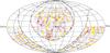 |
Fig. 1 Aitoff projection of galaxies in the 2M++ with a K-apparent magnitude lower than 12.5 (grey points) and excluding the region around the Galactic Plane (dashed lines). Open squares represent the 583 galaxy groups identified in the 2M++ catalogue using a contour overdensity contrast of 433 with a group radial velocity lower than 12 500 km s-1, and excluding galaxy groups that are closely related to CGs, while filled circles are the 63 2MCGs that lie in the restricted 2M++ area used in this work |
Recently, one of the largest samples of compact groups with confirmed membership using spectroscopic information has been extracted from the Two Micron All Sky Survey (2MASS; Skrutskie et al. 2006). Díaz-Giménez et al. (2012) have produced a very reliable sample of compact groups with several advantages: i) it is the largest available sample of velocity-filtered compact groups in the local Universe with at least four members of similar luminosity; ii) this sample has restricted the apparent magnitude of the brightest galaxy in the groups to ensure that all members can span a range of three magnitudes; iii) it is selected by stellar mass (K-band), which is expected to be a better tracer for magnitude gaps and luminosity segregation; and iv) this sample shows statistical signs of mergers; mergers are expected in physically dense groups. Therefore, this sample of compact groups gives us a very suitable opportunity to revisit the evidence about the location of these systems in the large-scale structure of the local Universe.
On the other hand, the statistical analyses performed for these peculiar systems using numerical simulations plus semi-analytic models of galaxy formation have been of great help in the last years. Among them are McConnachie et al. (2008) and Díaz-Giménez & Mamon (2010), who determined that between 50–70% of compact groups identified using Hickson’s criterion can be considered physically dense groups. They also demonstrated the incompleteness of the Hickson sample. Recently, and using similar semi-analytical tools, a new analysis of the influence of these extreme environments on their faint galaxy population has been performed by Zandivarez et al. (2014b). These authors reported that when compared with suitable control group samples, the compact group environment is not hostile enough to modify the distribution and density of the faint galaxy population that resides in the group and in their surroundings. Moreover, the authors also compared their results with those obtained using the observational sample of compact groups of Díaz-Giménez et al. (2012), which statistically confirmed their semi-analytical findings.
Therefore, the aim of this work is twofold: using the compact group sample extracted by Díaz-Giménez et al. (2012) from the 2MASS catalogue, we analyse the location of these systems in the underlying large scale structure traced by a new galaxy group sample extracted from the 2M++ catalogue; and we analyse whether the semi-analytical systems (compact and galaxy groups) extracted from a mock catalogue show a spatial distribution that resembles the results obtained from observations.
This paper is organised as follows: in Sect. 2 we describe the observational samples, that is, the catalogues and different procedures adopted to identify the compact groups and the galaxy groups. In Sect. 3 we determine the fraction of compact groups that can be considered as embedded systems, while in Sect. 4 we perform a similar analysis, but using compact and galaxy groups extracted from mock catalogues constructed from N-body simulations plus a semi-analytic model of galaxy formation. Finally, in Sect. 5 we summarise our results.
2. Samples
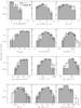 |
Fig. 2 Distributions of observable properties of observational and semi-analytical CGs. Number of members (top left panel), median radial velocity (top centre panel), difference in absolute magnitude between the brightest and the second brightest galaxies (top right panel), Ks-band apparent magnitude of the brightest galaxy member (second row, left panel), angular diameter of the smallest circle that encloses the galaxy members (second row, centre panel), projected group radius (second row, right panel), group surface brightness (third row, left panel), radial velocity dispersion (third row, centre panel), group virial radius (third row, right panel), dimensionless crossing time (bottom left panel), group virial mass (bottom centre panel), and mass-to-light ratio (bottom right panel). Grey shaded histograms correspond to the observational sample of CGs (2MCGs) that lie on the 2M++ restricted area, while black empty histograms correspond to semi-analytical CGs. Error bars correspond to Poisson errors. |
2.1. Compact group sample
We used the compact group sample (CGs) identified by Díaz-Giménez et al. (2012) in the 2MASS catalogue avoiding the Galactic plane (defined by Galactic latitude | b | ≤ 20). In this section, we briefly describe the procedure and the results found in that work.
The automated searching algorithm used in Díaz-Giménez et al. mimics the procedure defined by Hickson (1982), and their compact groups satisfy the criteria
-
4 ≤ N ≤ 10 (population),
-
μK ≤ 23.6 mag arcsec-2 (compactness),
-
ΘN> 3ΘG (isolation),
-
Kbrightest ≤ Klim − 3 = 10.57 (flux limit),
where N is the number of galaxies whose K-band magnitudes satisfy K<Kbrightest + 3, and Kbrightest is the apparent magnitude of the brightest galaxy of the group; μK is the mean K-band surface brightness, averaged over the smallest circle circumscribing the galaxy centres; ΘG is the angular diameter of the smallest circumscribed circle; ΘN is the angular diameter of the largest concentric circle that contains no other galaxies within the considered magnitude range or brighter. Using this algorithm and visual inspection, they found 230 CGs in the 2MASS XSC.
They also introduced a filtering of CGs according to velocity, that is, selecting CGs with | vi − ⟨ v ⟩ | ≤ 1000 km s-1, where vi is the radial velocity of each galaxy member and ⟨ v ⟩ is the median of the radial velocity of the members. Only 144 of the 230 CGs identified in projection had complete spectroscopic information. Of these, only 85 CGs passed the velocity filtering1.
We here used the sample of filtered 2MCGs selecting the 78 CGs with a median group velocity greater than 3000 km s-1 to avoid introducing effects of peculiar motions (see Díaz-Giménez et al. 2012 for further descriptions). We also restricted our sample to the area covered by the 2M++ catalogue (see next section for 2M++ description). The final sample comprises 63 CGs. The CG IDs of this sample are quoted in Table A.1. The sky coverage of these groups are shown as filled circles in Fig. 1. The distributions of different properties of CGs are shown as grey shaded histograms in Fig. 2. In this figure we show the distribution of the number of galaxy members in a range of three magnitudes from the brightest, median radial velocity (vcm), difference in K-band absolute magnitude between the brightest and second brightest galaxies in the group (K2 − K1), the K-band apparent magnitude of the brightest galaxy member (Kbrightest), the angular diameter of the smallest circle that encloses the galaxy members (ΘG), projected group radius of the smallest circle at the distance of the group centre (Rp), and the K-band group surface brightness (μK). We also show the radial velocity dispersion (σv) of compact groups computed using the gapper estimator described by Beers et al. (1990); the 3D group virial radius computed as  , given the inter-galaxy projected separations dij (see Eqs. (10)–(23) of Binney & Tremaine 1987); the dimensionless crossing time is computed as
 where ⟨ dij ⟩ is the median of the inter-galaxy projected separations in h-1 Mpc; and the virial masses that are obtained by applying the virial theorem (Limber & Mathews 1960),
  (1)Finally, we show the mass-to-light ratio where the group luminosity (LK) is computed by adding the individual galaxy luminosities obtained by using the K-correction given by Chilingarian et al. (2010). In the first column of Table A.2, we quote the median of these distributions and their semi-interquartile ranges.
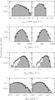 |
Fig. 3 Properties of galaxy groups. The distributions correspond to mean radial velocities (first row panels), radial velocity dispersions (second row panels), 3D virial radii (third row panels) and virial masses (fourth row panels) of GGs. Error bars correspond to Poisson errors. Shaded histograms show the distributions of properties of observational galaxy groups identified in the 2M++, while empty histograms show the same properties for mock galaxy groups identified in a 2M++ mock catalogue. The left column corresponds to the complete sample of galaxy groups identified by the FoF algorithm with a contour overdensity contrast of 433. The right column corresponds to the sample of galaxy groups with a radial velocity restricted to span the same range as compact groups and excluding the galaxy groups that can be considered as already included in the sample of compact groups. In this column, the mock GGs have been restricted to those that have more than four members after applying a blending criterion to account for the size of the particles (see Sect. 4.2). |
2.2. Galaxy group sample
To characterise the location of CGs in the local Universe we used as tracers a sample of galaxy groups (GGs) identified in the 2M++ galaxy redshift catalogue (Lavaux & Hudson 2011)2. This catalogue is based on the 2MASS photometric catalogue for target selection but with redshift information extracted from the NYU-VAGC for the Sloan Digital Sky Survey Data Release Seventh (SDSS-DR7, Abazajian & et al. 2009), the Six degree Field Data Release Three (6dF-DR3, Jones et al. 2009), and the Two Mass Redshift Survey (2MRS, Huchra et al. 2012).
Since the original 2M++ catalogue has a different magnitude coverage, we concentrated on the regions where K2M + + ≤ 12.5 covered by the SDSS-DR7 or 6dF-DR3, where K2M + + is the 2MASS Ks apparent magnitude corrected by galactic extinction, galaxy evolutionary effects, and aperture corrections (see Sect. 2.2 of Lavaux & Hudson 2011 for a complete description of the K2M + + magnitude). We also restricted the sample to galaxies outside the galactic plane (| b | > 20). The resulting galaxy sample comprises 52 982 galaxies. Their angular distribution in the sky is shown as grey points in Fig. 1.
The group identification was performed using a friends-of-friends (FoF) algorithm similar to that developed by Huchra & Geller (1982) to identify galaxy systems in redshift space in a flux-limited catalogue. The algorithm links galaxies that share common neighbours, that is, pairs of galaxies with projected separations smaller than D0 and radial velocity differences smaller than V0. Following the prescriptions of Zandivarez et al. (2014a), we used a radial linking length of V0 = 130 km s-1 and a transversal linking length, D0, defined by a contour overdensity contrast of δρ/ρ = 433 (see Eq. (4) in Huchra & Geller 1982). This value of δρ/ρ is adopted since it is expected that galaxies are more concentrated than dark matter (Eke et al. 2004; Berlind et al. 2006); therefore we should use a higher density contrast than that usually adopted in dark matter simulations, between 150–200 (see Appendix B of Zandivarez et al. 2014a for details).
Because of the flux limit of the galaxy sample, both linking lengths have to be weighted by a factor to take into account the variation of the sampling of the luminosity function produced by the different distances of the groups to the observers (see Eq. (3) of Huchra & Geller 1982). This factor is calculated using a Schechter fit of the galaxy luminosity function computed for the 2M++ galaxies by Lavaux & Hudson (2011): M∗ − 5log (h) = −23.43, α = −1.03, and n∗ = 0.0085 h3 Mpc-3. We computed the group physical properties: mean group radial velocity, radial velocity dispersions, 3D virial radii and virial masses (see Eq. (1) in the previous section and Sect. 5 of Merchán & Zandivarez 2002 for further descriptions).
We only selected groups with four or more members, mean group radial velocities greater than 3000 km s-1, and virial masses greater than 1012ℳ⊙h-1. The lower limit in mass is imposed to avoid galaxy groups with unreliable mass estimates given the errors in their velocity dispersions.
The final GG catalogue comprises 813 objects. The distribution of GG properties is shown as shaded histograms in the left column of Fig. 3. The sample has median radial velocity of 9829 km s-1, a median radial velocity dispersion of 172 km s-1, a median virial radius of 0.71 Mpc h-1, and median virial mass of 1.26 × 10¹³ℳ⊙h-1. This catalogue of galaxy groups is provided in Appendix B.
The FoF algorithm might identify some of the CGs as well as normal groups, and they might also be included in our sample of galaxy groups. We therefore examined the sample of galaxy groups to exclude these groups. First, we selected only the galaxies in GGs in a range of three magnitudes from its brightest member. Then, to determine whether a GG is also a CG, we imposed that at least 75% of the CG members have to be included in the GG, the number of members in the GG in a range of three magnitudes from the brightest has to be lower than twice the number of members in the CG, and only one of those GG member can lie outside the isolation ring (3ΘG). Based on this analysis, we discarded 12 GGs that are already included in the sample of CGs. The group-IDs of the discarded GGs are 11, 254, 308, 350, 357, 490, 503, 592, 642, 693, 741, and 775 (see first column of Tables B.1 and B.2 for references; in Table A.1 we flagged the CGs that matched these GGs).
It can be seen from Fig. 2 and the left column of Fig. 3 that CGs and GGs span different ranges of radial velocities. This difference is due to the brightest galaxy flux limit criterion imposed to identify CGs. Therefore, we also restricted the sample of GGs to those with radial velocities lower than 12 500 km s-1. The final sample comprises 583 galaxy groups. Their angular positions are shown as open squares in Fig. 1. The distributions of the main properties of the final GG sample are shown in the right column of Fig. 3, while the median of their properties are quoted in Table A.3.
3. Location of compact groups in reference to galaxy groups
As we stated in Sect. 1, nothing prevents CGs from being the core of normal groups or smaller substructures in loose groups or filaments. In this section we investigate how often this occurs in the local Universe. We analysed the location of CGs with respect to the location of GGs by classifying CGs into two subsamples: those located inside and those outside GGs (or isolated CGs).
Since we know the positions of CGs in redshift-space (2D+ ), the distortions in the line of sight of groups prevent studying 3D-distances between CGs and GGs. Therefore, we considered that a CG lies inside a given GG if the projected distance between the CG centre and the GG centre at the distance of the GG centre (dCG − GG) is smaller than the projected virial radius of the GG (
 ), and also the distance in the radial direction among centres (zCG − GG) is smaller than half the maximum line-of-sight separation among the galaxies identified as members of the GG (
 ), that is, CGs lie inside GGs if
 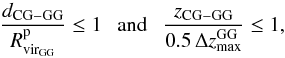 (2)where the centre of CGs and GGs in projected and radial directions are the barycentre of each system3. The scatter plot in Fig. 4 shows the distribution of all CG-GG normalised separations in the projected vs radial directions (grey points) as well as the distribution of CG-GG smallest normalised separations in the plane of sky (open black circles). The lower left region defined by the dashed lines in the scatter plot is the one we used to define embedded systems (Eq. (2)). As can be seen from the figure, selecting groups only by restricting the projected direction (i.e. projected normalised separation smaller than 1) is not enough to define embedded systems, since many of these systems are characterised by larger radial separations (i.e. radial normalised separation greater than 1). It is worth mentioning that the greatest projected distance we allowed to consider inside/outside GGs is a conservative value (
 ) since galaxies in groups may extend beyond that limit.
According to our definition, we found that 17 CGs inhabit GGs, that is, 27% of the sample of CGs. We recall that in the previous section, we have discarded 12 GGs because they matched some of the CGs in our sample. These 12 CGs that are also GGs represent 19% of the sample of CGs, hence, not including this constraint would have artificially increased the percentage of CGs located inside GGs.
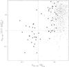 |
Fig. 4 Scatter plot of normalised projected and normalised radial separations between CGs and GGs. The grey points show all the separations from each CG to all GGs in the sample, while open black circles are the smallest CG-GG separations only selected in projection. The dashed lines indicate unity in the normalised distances. Embedded CGs lie in the lower left corner (see Eq. (2)). |
It is interesting to investigate if the global properties of the CGs are affected by their different environments. We analysed the distributions of properties of CGs embedded in GGs (27%) and those that could not be directly related to a GG (73%). We compared different properties using two statistical non-parametric tests: a Kolmogorov-Smirnov two-sample test and Mann-Whitney U test that measure the probability that both samples are drawn from the same distribution. In Table 1, we quote the p-values obtained from the two tests when comparing the properties of embedded and non-embedded CGs. Adopting a typical critical value of 0.05, we found that both tests indicate statistical differences for the distributions of group surface brightness and group projected radius (highlighted in boldface in Table 1). The embedded compact groups are typically brighter and smaller than their non-embedded counterparts.
P-values from two statistical two-sample tests to compare the properties of compact groups that can be considered embedded or not.
3.1. Subsamples of groups
We have also analysed whether different classes of CGs live preferentially inside GGs, and also if different properties of GGs make them more suitable to host CGs.
First, we split the sample of CGs according to the K-band absolute magnitude gap between the first ranked and the second ranked galaxies in the CG (K2 − K1, see Fig. 2). CGs whose magnitude gaps between the brightest and the second brightest galaxies are greater than or equal to the median of the K2 − K1 distribution are dominated by the brightest galaxy of the systems, and therefore we named this subsample dominated CGs. If the magnitude gap is smaller than the median of the distribution of differences, the CG is classified as non-dominated.
Another very important piece of information was obtained by analysing whether the embedded CGs are preferentially located in a particular type of GGs. To determine this, we split the sample of GGs according to their virial masses into low-, intermediate-, and high-mass groups using the 33th and the 66th percentiles of the mass distribution.
On the other hand, some of the CGs located inside GGs might be associated with a particular substructure of the host GG. Since the amount of substructure in GGs can be inversely associated with the level of relaxation of the groups (Einasto et al. 2012), one possible way to take into account this situation is to quantify the degree of equilibrium of a galaxy group by means of its galaxy member velocity distribution, that is, its internal dynamics. If the distribution has a Gaussian shape, then the system can be considered as relaxed, and a non-Gaussian shape of the velocity distribution is a strong indicator of the non-equilibrium state of the galaxy system. Hence, we split the sample of GGs according to the Gaussianity of the distributions of the radial velocities of their galaxy members. Following Martínez & Zandivarez (2012), we applied the Anderson-Darling goodness-of-fit test to distinguish between GGs with Gaussian or non-Gaussian velocity distributions, which can be understood as an indicator of the relaxation of the systems and the amount of substructure. For each group, the radial velocity of their members and the velocity dispersion of the group was used to compute a parameter, α (see Eqs. (7), (8), and (17) of Hou et al. 2009), to distinguish between Gaussian and non-Gaussian groups. However, according to Hou et al. (2009), this classification is statistically reliable only when the GG has five or more members, therefore, we only applied this test to the 329 GGs with Nmember ≥ 5. This subsample may include GGs that cannot be classified as Gaussian nor non-Gaussian.
To summarise, the subsamples of GGs are defined as follows:
-
Low-mass GGs: ℳvir ≤ 6 × 10¹² ℳ⊙h-1.
-
Intermediate-mass GGs: 6 × 10¹²ℳ⊙h-1< ℳvir< 1.48 × 10¹³ℳ⊙h-1.
-
High-mass GGs: ℳvir ≥ 1.48 × 10¹³ℳ⊙h-1.
-
Gaussian GGs: GGs with a Gaussian distribution of the radial velocity of their galaxy members, i.e., N ≥ 5 and α ≥ 0.5.
-
Non-Gaussian GGs: GGs with a non-Gaussian distribution of the radial velocity of their galaxy members, i.e., N ≥ 5 and α< 0.1.
-
Not classified (NC) GGs: GGs that cannot be classified as Gaussian or non-Gaussian, i.e., N ≥ 5 and 0.1 ≤ α< 0.5.
The number of groups belonging to each GG subsample and the median of their properties are quoted in Table A.3.
In Table 2, we quote the percentage of CGs that lie inside a GG. Each column corresponds to a subsample of CGs, while each row corresponds to a subsample of GGs. Errors are computed as the mean standard deviation of the percentages obtained from 100 bootstrap resamplings of the compact group subsample.
Percentages of compact groups that lie within the boundaries of galaxy groups in redshift-space.
The column labelled “ALL CG” of this table shows that (27 ± 5)% of the CGs are located inside GGs (first row). We first analysed the preference of the embedded CGs towards particular GG hosts divided according to the virial masses of the GGs. The percentage of CGs that inhabit different GG subsamples are quoted in the second, third, and fourth rows. We found that (6 ± 2)%, (14 ± 5)% and (6 ± 2)% of the CGs inhabit the low-, intermediate-, and high-mass GGs, respectively. We also included for each GG subsample the percentage of embedded CGs that would be expected if the distribution of embedded CGs were to depend only on the size of the GG subsamples. This expected percentage is computed as the product between the total percentage of embedded CGs and the percentage of each of the GG subsamples, quoted in the first column of Table 2. Errors for the expected values are computed via error propagation. The comparison between the measured and expected values shows that there is no preference (within 1 sigma significance level) of embedded CGs to inhabit any particular GG mass range subsample.
Secondly, we analysed the preference of the embedded CGs for a particular GG subsample split according to the Gaussianity of the distribution of the radial velocities of their members. We found that (26 ± 5)% of the CGs lie inside the GGs with five or more members that are used to split the GGs according to their dynamical state (see fifth row of the column labelled “ALL CG” in Table 2). By analysing the frequency of embedded CGs in Gaussian, non-Gaussian, and not-classified GGs and comparing these values with the expected ones, we found that there are no statistical indications that CGs prefer inhabiting GGs with any particular dynamical state.
Table 2 shows that about one third of the dominated CGs lies inside GGs, while only about one fifth of the non-dominated CGs are located in GGs. The comparison of the percentages of dominated and non-dominated CGs that inhabit different subsamples of GGs and the expected value shows no preferences of dominated and non-dominated embedded CGs to be located in GGs in a particular virial mass range or with a particular dynamical state.
4. Comparison with semi-analytical samples
We used a semi-analytic galaxy catalogue to perform the same analyses as were developed in the previous sections, with the aim of testing the current semi-analytic models of galaxy formation, and also to take advantage of the 3D information that we can access in the models and not in observations.
4.1. Mock catalogue
We adopted the mock all-sky galaxy light cone built by Henriques et al. (2012), which was constructed by replicating the Millennium I simulation box (500 Mpc h-1) and taking into account the evolution of structures by using the different outputs of the simulation at previous cosmological times4. The synthetic galaxies in this light cone were constructed using the semi-analytical model of galaxy formation developed by Guo et al. (2011). This mock catalogue provides the observer frame apparent magnitudes of galaxies in nine different bands, including the Ks-band, which we adopted in this work to perform the comparison with observations. We could have used the publicly available data from the Millennium II simulation combined with the same semi-analytical model, since it has a better resolution in mass. However, in a previous work (Díaz-Giménez & Mamon 2010), it has been shown that compact groups are dependent on the photometric band in which they are identified: a compact group in the K-band is not necessarily a compact group in the r-band. Since we are interested in comparing the results with those obtained from the 2MASS catalogue, we chose to work with the sample of Henriques et al. (2012) that has the K-band magnitudes available. It has also been shown that using the Millennium II or the Millennium I produces compact groups with very similar properties (Díaz-Giménez et al. 2012), the differences between the two simulations occur in a mass range that is beyond the scope of this work. We converted the apparent Ks(AB)-band available for the mock galaxies from the AB system to the Vega system to match the 2MASS magnitudes: Ks(Vega) = Ks(AB) − 1.85 (Blanton et al. 2005; Targett et al. 2012). We adopted an apparent magnitude limit of Ks = 13.57. The number density of this particular mock galaxy catalogue reproduces the number density observed in the 2MASS catalogue remarkably well.
4.2. Compact and galaxy group samples
We identified mock CGs in the galaxy light cone using the same criteria as described in Sect. 2.1, and following Díaz-Giménez & Mamon (2010), we also included the blending of galaxies in projection on the plane of the mock sky to take into account the fact that galaxies in the mock catalogue are point-sized particles. The main effect that the blending of galaxies has on the CG catalogue is in the number of members that we are able to detect, which is important since one of the criteria for identifying CGs is indeed the membership (population). In that previous work, the authors have used the prescriptions of Shen et al. (2003) to compute the half-light radii as a function of the absolute magnitude in the r-band of each mock galaxy. They blended two galaxies if their angular separation was smaller than the sum of their angular half-light radii. Motivated by some differences between SAMs and observations pointed out in previous works, mainly regarding the space density and the projected sizes of CGs, we here slightly changed the criterion to improve the comparison between the observational and mock samples of CGs. First, we split the galaxies into ellipticals and non-ellipticals. Following Bertone et al. (2007), we used the ratio between the bulge mass and the total stellar mass provided by the semi-analytical model as a proxy for the morphology of our mock galaxies. We classified as ellipticals the galaxies with more than 70 per cent of their stars in the bulge, the remaining galaxies were classified as non-ellipticals. Then, we used the prescriptions of Lange et al. (2015) to compute the half-light radius of each mock galaxy in the K-band as a function of the stellar mass of each mock galaxy (see Eq. (2) for non-ellipticals and Eq. (3) for ellipticals in that work). Finally, we considered two galaxies as blended if the angular separation between the two galaxies is smaller than one and a half times the sum of their angular half-light radii.
We identified 380 CGs within a solid angle of 4π. Then, we restricted the sample to the area covered by the 2M++ catalogue and excluded the CGs with radial velocities lower than 3000 km s-1, as we did with observations. We also discarded the mock CGs that had more than six members to match the observations (top left panel of Fig. 2). The final sample comprises 150 mock CGs. The distributions of CG properties are shown as empty histograms in Fig. 2. To compare the properties of observable and mock CGs, the Kolmogorov-Smirnov and Man-Whitney U-test probabilities are quoted in Table 3. In general, the properties of observed CGs are well recovered in the mock catalogue, although in the semi-analytic CGs we found an excess of CGs that were dominated by a bright galaxy (high K2 − K1) and had a lower group virial radius. The differences in these distributions are not as significant as was previously reported (Díaz-Giménez & Mamon 2010; Díaz-Giménez et al. 2012). On one hand, we checked that discarding the mock CGs with a multiplicity higher than the observed multiplicity produced a mock CG sample more similar to the observations in all the other properties. The absence of high-multiplicity CGs in the observed 2MCG sample might only be a limitation imposed by the lack of redshift measurements for all the galaxies in the 2MASS catalogue. On the other hand, the stronger criterion for blending galaxies than the one used in previous works can better account for the observational effect.
P-values from different statistical two-sample tests to compare the properties of compact groups obtained from observations and from a mock galaxy catalogue.
The GG sample was identified with the FoF algorithm described in Sect. 2.2 applied on the mock galaxy catalogue with the same sky coverage as the 2M++ sample, and having galaxies brighter than K2M + + = 12.5, where K2M + + is the apparent magnitude of the mock catalogue corrected in a similar way as in the original 2M++ catalogue, but in this case only corrected by k-correction and galaxy evolutionary effects: K2M + + = Ks + 1.16 (2.1 z + 0.8 z) (Lavaux & Hudson 2011).
We identified 1065 GGs with a contour overdensity contrast of 433, virial masses higher than 1012 ℳ⊙h-1, mean radial velocities greater than 3000 km s-1, and with four or more members. The property distributions are shown as empty histograms in the left column of Fig. 3. In comparison with the observational sample of GGs, the mock GGs tend to have smaller virial radii, and hence, the virial mass distribution is slightly shifted towards lower virial masses. We then recomputed the membership of each group after applying the blending criterion described at the beginning of this section and discarded groups with fewer than four galaxies after blending. Finally, following a similar procedure as the one performed in the observational sample, we discarded 32 mock GGs that are also CGs and restricted the GG sample to those with radial velocities lower than 12 500 km s-1. The final sample comprises 770 mock GGs. The property distributions are shown as empty histograms in the right column of Fig. 3, while the median of their properties are quoted in Table A.3. The statistical comparison between the mock and observational GGs performed with KS and Mann-Whitney U test confirms differences in the virial radii: the mock GGs are smaller than the observational sample. Nevertheless, the comparison between mock and observational results in respect to the analysis of the location of CGs with respect to GGs is not affected by the sizes of GGs since we used distances normalised to the virial radii to avoid introducing a dependence on the sizes of the groups (Eq. (2)).
4.3. Location of compact groups in redshift space
We examined the distribution of mock CGs in relation to mock GGs by analysing the percentages of CGs that are located in GGs following the criterion specified in Eq. (2).
We split the samples of CGs and GGs into the different subsamples defined in Sect. 3.1, but we also introduced a new classification for CGs by using the 3D information (in real space) available in the simulation. Following Díaz-Giménez & Mamon (2010), we split the sample of CGs into physically dense CGs (Reals) and chance alignments (CAs). Reals and CAs were defined based on the physical separations between the four closest galaxies. Real CGs satisfy s4 ≤ 100 kpc h-1 or (s4 ≤ 200 kpc h-1 and S∥/S⊥ ≤ 2), where s4 is the largest interparticle separation in real space between the four closest galaxies (or the CG itself for quartets), S∥ is the largest projected separation, and S⊥ is the largest separation in the line of sight of the four closest galaxies in the CG. Using this definition, we found that 54% (pR) of the mock CGs are Reals.
The numbers of CGs in each of the subsamples and the median of some of their properties are quoted in Table A.2. The number and the median of the properties of each of the GGs are quoted in Table A.3.
The results of the location of mock CGs compared to mock GGs are quoted in Table 2. The percentage of CGs that lie inside GGs (pe = 27%) in the mock catalogue is the same as the percentage found in the observational sample. This result is very encouraging since it confirms the capability of the current models of galaxy formation to reproduce the observations of these peculiar environments. We analysed the distribution of properties of CGs that lie inside and outside GGs. The results from the statistical tests are quoted in Table 1. We found significant differences in the distributions of radial velocities, dominance of the brightest galaxy, surface brightnesses, projected radii, group virial radii and crossing times, with the embedded CGs having brighter surface brightnesses, smaller sizes, and shorter crossing times. The observations also present similar differences in surface brightnesses and projected radii. This means that observational and semi-analytical results indicate that embedded CG are typically smaller in size and brighter than non-embedded CGs.
From Table 2, analysing the column labelled “ALL CG”, our results show that the mock CGs that inhabit GGs do not have a statistical preference towards GGs in any particular mass range, in agreement with the results from observations. In addition, mock CGs that inhabit GGs with five or more members do not have a preference to inhabit GGs with a particular dynamical state (Gaussian/non-Gaussian/not classified).
Some discrepancies can also be observed in the percentages of dominated and non-dominated CGs that lie inside GGs compared with the observational results. In the mock samples, dominated CGs are less frequent in embedded systems than non-dominated CGs (22% and 32%), but in observations it is the other way around, dominated CGs are more likely to inhabit GGs than non-dominated (34% vs. 19%). However, when analysing the different subsamples of GGs, neither observational or mock dominated/non-dominated CGs show any preferences within 1 sigma significance level.
Finally, the last two columns of Table 2 show a piece of information that we can only access from simulations: there is a larger percentage of physically dense CGs that lie inside GGs ( ) than the corresponding percentage obtained for CGs considered chance alignments (
 ). Since the definitions of Reals and CAs can only be made from simulations, it is useful to seeking observational clues that can help us select subsamples of CGs that are dominated by physically dense systems. By using the previous results, we can predict the percentage of embedded compact groups that are Reals. This percentage can be computed as
  . On the other hand, performing the same calculation for the non-embedded CGs, we found that the percentage of non-embedded CGs that are Reals is
  . Therefore, the non-embedded CGs comprise similar percentages of Reals and CAs. Hence, this result is very useful as a selection criterion in an observational sample of CGs that are more likely to be Real. Assuming that this prediction can be applied to observations, by selecting a sample of embedded CGs we can obtain a sample of CGs where roughly two-thirds of the sample can be considered physically dense systems. Applied to 2MCGs, from the 17 2MCGs that are embedded in GGs, we expect 12 of them to be Real CGs.
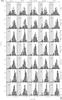 |
Fig. 5 Distributions of the 3D smallest normalised separation in real space between compact and galaxy groups (dark grey histograms). Each column represents a different subsample of CGs, each row represents a different GG subsample. Each panel also shows the distribution of the 3D smallest separation in real space among the GGs (black empty histogram). The light-grey region in each panel determines the inner region of a GG. Inside that region we quote the percentage of compact groups that are expected to lie inside a GG (see Sect. 3.1 for a more detailed description of each subsample). |
Finally, taking into account the expected values computed from the relative abundances of GG subsamples, we found that Reals and CAs are equally distributed within each GG subsample.
4.4. Location of compact groups in real space
Because real space information is available in the mock catalogue, in this section we explore the location of CGs around GGs in the mock catalogue when the redshift distortions are avoided.
For each mock CG, we computed the 3D (in real space) comoving distance to its closest GG. The smallest separation between CGs and GGs was computed by the Euclidean distance between two points in real space (rmin). For the sake of comparison, we also computed the smallest separation among normal groups. We normalised the distances by the 3D virial radius of the closest GG.
The top left panel of Fig. 5 shows as grey histogram the distribution of the normalised smallest distances of CGs to GGs. In this figure, the empty histogram is the distribution of normalised smallest distances of GGs to GGs. The light-grey area represents the region inside unity in the normalised distances. The number quoted inside this region is the percentage of CGs whose smallest distance to a GG is smaller than unity, that is, they are positioned inside the virial radius of their closest GG neighbour.
It can be seen from the top left panel of this figure that 27% of the CGs can be considered as located inside one virial radius of its closest GG neighbour in real space. This result agrees with what we found in the previous sections. Hence, this indicates that our criterion to define what is inside or outside in the distorted redshift space is indeed representative of the behaviour in real space. Moreover, almost all the percentages quoted in this figure are quite similar to those obtained in redshift space for all the subsamples under analysis.
Finally, the real space information allowed us also to reach a wider understanding of the location of CGs around GGs in the Universe. We found that for most of the subsamples of CGs, the distribution of distances of CGs to the complete sample of GGs (first row) is clearly bimodal and clearly distinguishable from the distribution of distances of GG-GG, except for the chance alignment CGs, which behave similarly to the GG-GG distribution. Although this analysis cannot be made in observations, hints of this behaviour can be obtained from Fig. 4, which shows a concentration of points in two different regions of this scatter plot (bottom left and top right corner).
5. Summary and conclusions
We analysed the location of compact groups in the local Universe to determine how important their environment is for the formation scenario of these systems and for the properties of their galaxy members. We used two different approaches, an observational and a semi-analytical one.
For the observational case, we adopted the compact group catalogue extracted from the 2MASS catalogue by Díaz-Giménez et al. (2012). This sample has proved to be a very useful tool since it is one of the largest catalogues with spectroscopically confirmed compact groups and homogeneity in the selection of the galaxy members that form the groups, it also shows strong statistical evidence of mergers at the bright end and luminosity segregation. We adopted as tracer of the large-scale structure of the local Universe a new sample of galaxy groups identified in the 2M++ galaxy redshift catalogue with a contour overdensity contrast of 433. This galaxy group sample differs from the sample published by Lavaux & Hudson (2011) with a contour overdensity contrast of 80, although the algorithm to identify both is similar (Friends-of-Friends). Following previous works (Eke et al. 2004; Berlind et al. 2006; Zandivarez et al. 2014a,b), we adopted a higher contour overdensity contrast to identify galaxy groups in an observational galaxy catalogue.
To perform a comparison with results obtained using mock catalogues, we adopted the available light cone mock catalogue constructed by Henriques et al. (2012) using the Millennium I simulation plus the semi-analytical model of galaxy formation developed by Guo et al. (2011). We adapted this mock catalogue to mimic the main characteristics of the 2MASS and the 2M++ observational catalogues (sky coverage and flux limit) and proceeded to construct mock compact and galaxy group samples following the same procedures as used in the observations.
To distinguish between compact groups that lie inside or outside galaxy systems in redshift space, we defined a criterion that takes into account separations in both directions, projected and radial. Based on our computations using the observational samples, we obtained that only 27% of compact groups can be considered to be embedded in overdense systems, that is, compact groups are more likely to be isolated from galaxy groups. This result is lower than the ~50% obtained by Andernach & Coziol (2005), Mendel et al. (2011) and better agrees with Palumbo et al. (1995), de Carvalho et al. (2005), who found percentages ranging from ~20% to ~30%. One source for the discrepancy with some of the previous works could arise from the way our compact group sample was selected: only compact groups whose brightest galaxy was fainter than three magnitudes from the magnitude limit of the source catalogue were considered. Defining a compact group sample without this restriction includes systems that might not fulfil the membership, or the isolation or the compactness criteria that might artificially increase the fraction of embedded compact groups. Another source might be that we carefully selected the galaxy group sample to avoid considering galaxy groups that are actually compact groups. We demonstrated that the samples of compact groups and galaxy groups have an intersection of 12 groups (which represents 19% of the 2MCGs and 2% of the galaxy groups). If we had not eliminated these groups from the galaxy group sample, we would have artificially increased the percentage of embedded compact groups, finding that 46% of the compact group sample are embedded in larger structures, similar to the previously reported findings.
We compared the properties of embedded and non-embedded compact groups. We found differences in the distributions of surface brightness and projected radius, with a tendency of the embedded compact groups to be brighter and smaller than the non-embedded compact groups.
We also extended the results by analysing different subsamples of compact and galaxy groups to determine where those embedded compact groups are more likely to be found. We observed that embedded compact groups are equally likely to be found in groups within any virial mass range. Moreover, using the radial velocity distribution of the group galaxy members to characterise the dynamical state of the host galaxy groups, we found no significant evidence supporting the idea that embedded compact groups are more likely to reside in galaxy groups that have not reached dynamical equilibrium. Nevertheless, owing to the low number of groups with non-Gaussian distribution in our sample, these results need to be confirmed with larger samples to increase the statistical significance of our findings.
When dividing compact groups according to the dominance of the brightest galaxy (using the magnitude gap between the first and second brightest galaxies), we also observed that about one third of the dominated compact groups lies inside galaxy groups, while only about one fifth of the non-dominated compact groups are embedded systems. Neither the embedded dominated nor non-dominated compact groups show preferences to inhabit galaxy systems within a particular virial mass range.
After performing a similar analysis on samples of compact and galaxy groups extracted from a mock galaxy catalogue with semi-analytic information, we observed that the percentages of embedded mock compact groups in redshift space agree very well with those obtained from the observations. Moreover, in both observed and mock compact groups, we found that the embedded compact groups tend to be smaller and brighter than the non-embedded compact groups. The semi-analytic catalogue is also able to reproduce the results found in observations regarding the independence of embedded compact groups to inhabit galaxy groups of any virial mass and dynamical state. On the other hand, we found that mock dominated compact groups are less likely to inhabit galaxy groups than observational dominated compact groups, while mock non-dominated compact groups are more likely to be found embedded in galaxy groups than the observational non-dominated compact groups. Since the observational sample of compact groups was constructed based on the public availability of radial velocities of the group members, there might be a bias towards finding dominated compact groups (a large galaxy surrounded by small galaxies) preferentially inhabiting groups, which are the regions that could be more uniformly sampled, and therefore, the fraction of embedded dominated compact groups is artificially higher than in the mock catalogue. The observational embedded non-dominated compact groups might also have been lost because of the blending of two similar galaxies located in an overdense environment. Although we intended to reproduce the observational blending of galaxies in the mock catalogue, it might not be enough.
We also split the compact groups in the mock catalogue according to a criterion defined by Díaz-Giménez & Mamon (2010) to classify these systems into 3D physically dense or chance alignment compact groups. From this analysis, we obtained that the percentage of physically dense compact groups that are embedded in galaxy groups is higher than the percentage of embedded chance alignments. We found that the embedded compact groups are dominated by physically dense systems (~70%), while non-embedded compact groups comprise similar percentages of real and chance alignment compact groups. Therefore, this prediction from the semi-analytical sample can be used as a proxy to obtain a subsample of compact groups dominated by physically dense systems. Eigthy-three percent of the chance alignment compact groups are not embedded in galaxy groups. This discourages the idea of chance alignment compact groups being projections inside loose groups. They might still be projections inside filaments or the field , however.
Finally, we used the real space information of the mock catalogue and computed the distribution of 3D minimum normalised compact group-galaxy group separations for each subsample previously analysed in redshift space. We found an overall very good agreement with the percentages of embedded compact groups obtained by the analysis in redshift space. These results clearly support our criterion of defining the smallest separation in redshift space. Moreover, by analysing the distribution of normalised distances, we observed that the shape of the distribution are bimodal for several of the subsample combinations, which might be an indication that these are compact groups that may have followed different evolutionary paths depending on the regions they inhabit.
We conclude that the location of compact groups needs to be carefully taken into account when comparing properties of galaxies in compact groups vs galaxies in different environments such as normal groups. Compact groups that are also identified as normal groups with the usual group-searching algorithms and compact groups that are embedded in normal systems constitute almost half of the sample of compact groups. If they are not excluded from the galaxy group sample, the comparison of these samples of galaxy systems will be biased by the large intersection among them. Moreover, if embedded and non-embedded compact groups are not distinguished, the results might be biased as well because both types of compact groups might be intrinsically different, showing different properties, such as the smaller sizes of embedded compact groups, which might be related with different formation scenarios.
As a by-product, we release a new galaxy group catalogue extracted from the 2M++ catalogue that will be available at the CDS for the astronomical community (see Appendix B for details).
Online material
Appendix A: Properties of compact groups and galaxy groups
In Table A.1 we list the group IDs of compact groups identified by Díaz-Giménez et al. (2012) that have been used in this work. The list includes only the 63 compact groups with radial velocities higher than 3000 km s-1 and within the sky coverage of the 2M++ catalogue. The complete catalogue is available at VizieR – cat. J/MNRAS/426/296.
In Table A.2 we quote the median and semi-interquartile ranges of several properties of observational and mock compact groups, split into different subsamples.
In Table A.3 we quote the median and semi-interquartile ranges of several properties of observational and mock galaxy groups, split into different subsamples.
Compact groups from the 2MCG catalogue.
Properties of compact groups in different subsamples: median and semi-interquartile ranges.
Properties of galaxy groups in different subsamples: median and semi-interquartile ranges.
Appendix B: Group catalogue with δρ/ρ = 433
In this section we quote the content of the tables of galaxy groups identified in the 2M++ catalogue using a contour overdensity contrast of 433. In Table B.1 we show part of the table containing the 813 galaxy groups, while Table B.2 shows also part of the table that quotes the information for the 4869 galaxy members.
Galaxy groups identified in the 2M++ catalogue (Lavaux & Hudson 2011).
Galaxy members of groups identified in the 2M++ catalogue (Lavaux & Hudson 2011).
Catalogue available at VizieR – cat. J/MNRAS/426/296.
Catalogue available at VizieR – cat. J/MNRAS/416/2840.
For CGs, the projected centre is usually assumed to be the centre of the smallest circle. However, we adopted the barycentre to match the procedure used for GGs.
Galaxy mock light cone available as table wmap1.BC03_ AllSky_001 at http://www.mpa-garching.mpg.de/millennium/
Acknowledgments
We acknowledge the anonymous referee for insightful comments and suggestions that increased the general quality of the paper. This publication makes use of data products from the Two Micron All Sky Survey, which is a joint project of the University of Massachusetts and the Infrared Processing and Analysis Center/California Institute of Technology, funded by the National Aeronautics and Space Administration and the National Science Foundation. The Millennium Simulation databases used in this paper and the web application providing online access to them were constructed as part of the activities of the German Astrophysical Virtual Observatory (GAVO). We thank Bruno Henriques for allowing public access for his galaxy light cones and for kindly answering questions about the data. This work has been partially supported by Consejo Nacional de Investigaciones Científicas y Técnicas de la República Argentina (CONICET), Secretaría de Ciencia y Tecnología de la Universidad de Córdoba (SeCyT)
References
- Abazajian, K. N., Adelman-McCarthy, J. K., Agüeros, M. A., et al. 2009, ApJS, 182, 543 [NASA ADS] [CrossRef] [Google Scholar]
- Adelman-McCarthy, J. K., Agüeros, M. A., Allam, S. S., et al. 2008, ApJS, 175, 297 [NASA ADS] [CrossRef] [Google Scholar]
- Andernach, H., & Coziol, R. 2005, in Nearby Large-Scale Structures and the Zone of Avoidance, eds. A. P. Fairall, & P. A. Woudt, ASP Conf. Ser., 329, 67 [Google Scholar]
- Baier, F. W., & Tiersch, H. 1975, Astrofizika, 11, 221 [NASA ADS] [Google Scholar]
- Baier, F. W., & Tiersch, H. 1976a, Astrofizika, 12, 7 [NASA ADS] [Google Scholar]
- Baier, F. W., & Tiersch, H. 1976b, Astrofizika, 12, 409 [NASA ADS] [Google Scholar]
- Baier, F. W., & Tiersch, H. 1978, Astrofizika, 14, 279 [Google Scholar]
- Baier, F. W., & Tiersch, H. 1979, Astrofizika, 15, 33 [NASA ADS] [Google Scholar]
- Baier, F. W., Petrosian, M. B., Tiersch, H., & Shakbazyan, R. K. 1974, Astrofizika, 10, 327 [NASA ADS] [Google Scholar]
- Barton, E., Geller, M., Ramella, M., Marzke, R. O., & da Costa, L. N. 1996, AJ, 112, 871 [NASA ADS] [CrossRef] [Google Scholar]
- Barton, E. J., de Carvalho, R. R., & Geller, M. J. 1998, AJ, 116, 1573 [NASA ADS] [CrossRef] [Google Scholar]
- Beers, T. C., Flynn, K., & Gebhardt, K. 1990, AJ, 100, 32 [NASA ADS] [CrossRef] [Google Scholar]
- Berlind, A. A., Frieman, J., Weinberg, D. H., et al. 2006, ApJS, 167, 1 [NASA ADS] [CrossRef] [Google Scholar]
- Bertone, S., De Lucia, G., & Thomas, P. A. 2007, MNRAS, 379, 1143 [NASA ADS] [CrossRef] [Google Scholar]
- Binney, J., & Tremaine, S. 1987, Galactic Dynamics (Princeton, NJ: Princeton University Press) [Google Scholar]
- Blanton, M. R., Schlegel, D. J., Strauss, M. A., et al. 2005, AJ, 129, 2562 [NASA ADS] [CrossRef] [Google Scholar]
- Chilingarian, I. V., Melchior, A.-L., & Zolotukhin, I. Y. 2010, MNRAS, 405, 1409 [NASA ADS] [CrossRef] [Google Scholar]
- Coenda, V., Muriel, H., & Martínez, H. J. 2012, A&A, 543, A119 [NASA ADS] [CrossRef] [EDP Sciences] [Google Scholar]
- de Carvalho, R., de La Rosa, I., & Zepf, S. 2003, Ap&SS, 285, 79 [NASA ADS] [CrossRef] [Google Scholar]
- de Carvalho, R. R., Gonçalves, T. S., Iovino, A., et al. 2005, AJ, 130, 425 [NASA ADS] [CrossRef] [Google Scholar]
- de la Rosa, I. G., de Carvalho, R. R., Vazdekis, A., & Barbuy, B. 2007, AJ, 133, 330 [NASA ADS] [CrossRef] [Google Scholar]
- del Olmo, A., Moles, M., & Perea, J. 1995, ASPC, 70, 117 [NASA ADS] [Google Scholar]
- Díaz-Giménez, E., & Mamon, G. A. 2010, MNRAS, 409, 1227 [NASA ADS] [CrossRef] [Google Scholar]
- Díaz-Giménez, E., Mamon, G. A., Pacheco, M., Mendes de Oliveira, C., & Alonso, M. V. 2012, MNRAS, 426, 296 [NASA ADS] [CrossRef] [Google Scholar]
- Einasto, M., Vennik, J., Nurmi, P., et al. 2012, A&A, 540, A123 [NASA ADS] [CrossRef] [EDP Sciences] [Google Scholar]
- Eke, V. R., Baugh, C. M., Cole, S., et al. 2004, MNRAS, 348, 866 [NASA ADS] [CrossRef] [Google Scholar]
- Focardi, P., & Kelm, B. 2002, A&A, 391, 35 [NASA ADS] [CrossRef] [EDP Sciences] [Google Scholar]
- Guo, Q., White, S., Boylan-Kolchin, M., et al. 2011, MNRAS, 413, 101 [NASA ADS] [CrossRef] [Google Scholar]
- Henriques, B. M. B., White, S. D. M., Lemson, G., et al. 2012, MNRAS, 421, 2904 [NASA ADS] [CrossRef] [Google Scholar]
- Hernquist, L., Katz, N., & Weinberg, D. H. 1995, ApJ, 442, 57 [NASA ADS] [CrossRef] [Google Scholar]
- Hickson, P. 1982, ApJ, 255, 382 [NASA ADS] [CrossRef] [Google Scholar]
- Hickson, P. 1997, ARA&A, 35, 357 [NASA ADS] [CrossRef] [Google Scholar]
- Hickson, P., & Rood, H. J. 1988, ApJ, 331, L69 [NASA ADS] [CrossRef] [Google Scholar]
- Hou, A., Parker, L. C., Harris, W. E., & Wilman, D. J. 2009, ApJ, 702, 1199 [NASA ADS] [CrossRef] [Google Scholar]
- Huchra, J. P., & Geller, M. J. 1982, ApJ, 257, 423 [NASA ADS] [CrossRef] [Google Scholar]
- Huchra, J. P., Macri, L. M., Masters, K. L., et al. 2012, ApJS, 199, 26 [NASA ADS] [CrossRef] [Google Scholar]
- Jones, D. H., Read, M. A., Saunders, W., et al. 2009, MNRAS, 399, 683 [NASA ADS] [CrossRef] [Google Scholar]
- Kelm, B., & Focardi, P. 2004, A&A, 418, 937 [NASA ADS] [CrossRef] [EDP Sciences] [Google Scholar]
- Krusch, E., Bomans, D. J., Dettmar, R.-J., & Taylor, C. 2003, BAAS, 35, 1288 [NASA ADS] [Google Scholar]
- Lange, R., Driver, S. P., Robotham, A. S. G., et al. 2015, MNRAS, 447, 2603 [NASA ADS] [CrossRef] [Google Scholar]
- Lavaux, G., & Hudson, M. J. 2011, MNRAS, 416, 2840 [NASA ADS] [CrossRef] [Google Scholar]
- Lee, B. C., Allam, S. S., Tucker, D. L., et al. 2004, AJ, 127, 1811 [NASA ADS] [CrossRef] [Google Scholar]
- Limber, D. N., & Mathews, W. G. 1960, ApJ, 132, 286 [NASA ADS] [CrossRef] [Google Scholar]
- Mamon, G. A. 1986, ApJ, 307, 426 [NASA ADS] [CrossRef] [Google Scholar]
- Martínez, H. J., & Zandivarez, A. 2012, MNRAS, 419, L24 [Google Scholar]
- Martinez, M. A., del Olmo, A., Coziol, R., & Perea, J. 2010, AJ, 139, 1199 [NASA ADS] [CrossRef] [Google Scholar]
- Martínez, H. J., Coenda, V., & Muriel, H. 2013, A&A, 557, A61 [NASA ADS] [CrossRef] [EDP Sciences] [Google Scholar]
- McConnachie, A. W., Ellison, S. L., & Patton, D. R. 2008, MNRAS, 387, 1281 [NASA ADS] [CrossRef] [Google Scholar]
- McConnachie, A. W., Patton, D. R., Ellison, S. L., & Simard, L. 2009, MNRAS, 395, 255 [NASA ADS] [CrossRef] [Google Scholar]
- Mendel, J. T., Ellison, S. L., Simard, L., Patton, D. R., & McConnachie, A. W. 2011, MNRAS, 418, 1409 [NASA ADS] [CrossRef] [Google Scholar]
- Mendes de Oliveira, C., & Hickson, P. 1991, ApJ, 380, 30 [NASA ADS] [CrossRef] [Google Scholar]
- Merchán, M., & Zandivarez, A. 2002, MNRAS, 335, 216 [NASA ADS] [CrossRef] [Google Scholar]
- Moles, M., del Olmo, A., Perea, J., et al. 1994, A&A, 285, 404 [NASA ADS] [Google Scholar]
- Palumbo, G. G. C., Saracco, P., Hickson, P., & Mendes de Oliveira, C. 1995, AJ, 109, 1476 [NASA ADS] [CrossRef] [Google Scholar]
- Petrosian, M. B. 1974, Astrofizika, 10, 471 [NASA ADS] [Google Scholar]
- Petrosian, M. B. 1978, Astrofizika, 14, 631 [NASA ADS] [Google Scholar]
- Plauchu-Frayn, I., del Olmo, A., Coziol, R., & Torres-Papaqui, J. P. 2012, A&A, 546, A48 [NASA ADS] [CrossRef] [EDP Sciences] [Google Scholar]
- Prandoni, I., Iovino, A., & MacGillivray, H. T. 1994, AJ, 107, 1235 [NASA ADS] [CrossRef] [Google Scholar]
- Proctor, R. N., Forbes, D. A., Hau, G. K. T., et al. 2004, MNRAS, 349, 1381 [NASA ADS] [CrossRef] [Google Scholar]
- Robinson, L. B., & Wampler, E. J. 1973, ApJ, 179, L35 [Google Scholar]
- Rood, H. J., & Struble, M. F. 1994, PASP, 106, 413 [NASA ADS] [CrossRef] [Google Scholar]
- Rose, J. A. 1977, ApJ, 211, 311 [NASA ADS] [CrossRef] [Google Scholar]
- Seyfert, C. K. 1948, AJ, 53, 203 [NASA ADS] [CrossRef] [Google Scholar]
- Shakbazyan, R. K. 1973, Astrofizika, 9, 495 [NASA ADS] [Google Scholar]
- Shakbazyan, R. K., & Petrosian, M. B. 1974, Astrofizika, 10, 13 [NASA ADS] [Google Scholar]
- Shen, S., Mo, H. J., White, S. D. M., et al. 2003, MNRAS, 343, 978 [NASA ADS] [CrossRef] [Google Scholar]
- Skrutskie, M. F., Cutri, R. M., Stiening, R., et al. 2006, AJ, 131, 1163 [NASA ADS] [CrossRef] [Google Scholar]
- Stephan, M. 1877, MNRAS, 37, 334 [NASA ADS] [CrossRef] [Google Scholar]
- Targett, T. A., Dunlop, J. S., & McLure, R. J. 2012, MNRAS, 420, 3621 [NASA ADS] [CrossRef] [Google Scholar]
- Tovmassian, H. M., Yam, O., & Tiersch, H. 2001, Rev. Mex. Astron. Astrofis., 37, 173 [NASA ADS] [Google Scholar]
- Verdes-Montenegro, L., del Olmo, A., Perea, J., et al. 1994, A&A, 321, 409 [Google Scholar]
- Verdes-Montenegro, L., Yun, M. S., Williams, B. A., et al. 2001, A&A, 377, 812 [NASA ADS] [CrossRef] [EDP Sciences] [Google Scholar]
- Verdes-Montenegro, L., del Olmo, A., Yun, M. S., & Perea, J. 2005, A&A, 430, 443 [NASA ADS] [CrossRef] [EDP Sciences] [Google Scholar]
- Zandivarez, A., Díaz-Giménez, E., Mendes de Oliveira, C., et al. 2014a, A&A, 561, A71 [NASA ADS] [CrossRef] [EDP Sciences] [Google Scholar]
- Zandivarez, A., Diaz-Gimenez, E., Mendes de Oliveira, C., & Gubolin, H. 2014b, A&A, 572, A68 [NASA ADS] [CrossRef] [EDP Sciences] [Google Scholar]
All Tables
P-values from two statistical two-sample tests to compare the properties of compact groups that can be considered embedded or not.
Percentages of compact groups that lie within the boundaries of galaxy groups in redshift-space.
P-values from different statistical two-sample tests to compare the properties of compact groups obtained from observations and from a mock galaxy catalogue.
Properties of compact groups in different subsamples: median and semi-interquartile ranges.
Properties of galaxy groups in different subsamples: median and semi-interquartile ranges.
Galaxy members of groups identified in the 2M++ catalogue (Lavaux & Hudson 2011).
All Figures
|
Fig. 1 Aitoff projection of galaxies in the 2M++ with a K-apparent magnitude lower than 12.5 (grey points) and excluding the region around the Galactic Plane (dashed lines). Open squares represent the 583 galaxy groups identified in the 2M++ catalogue using a contour overdensity contrast of 433 with a group radial velocity lower than 12 500 km s-1, and excluding galaxy groups that are closely related to CGs, while filled circles are the 63 2MCGs that lie in the restricted 2M++ area used in this work |
| In the text | |
|
Fig. 2 Distributions of observable properties of observational and semi-analytical CGs. Number of members (top left panel), median radial velocity (top centre panel), difference in absolute magnitude between the brightest and the second brightest galaxies (top right panel), Ks-band apparent magnitude of the brightest galaxy member (second row, left panel), angular diameter of the smallest circle that encloses the galaxy members (second row, centre panel), projected group radius (second row, right panel), group surface brightness (third row, left panel), radial velocity dispersion (third row, centre panel), group virial radius (third row, right panel), dimensionless crossing time (bottom left panel), group virial mass (bottom centre panel), and mass-to-light ratio (bottom right panel). Grey shaded histograms correspond to the observational sample of CGs (2MCGs) that lie on the 2M++ restricted area, while black empty histograms correspond to semi-analytical CGs. Error bars correspond to Poisson errors. |
| In the text | |
|
Fig. 3 Properties of galaxy groups. The distributions correspond to mean radial velocities (first row panels), radial velocity dispersions (second row panels), 3D virial radii (third row panels) and virial masses (fourth row panels) of GGs. Error bars correspond to Poisson errors. Shaded histograms show the distributions of properties of observational galaxy groups identified in the 2M++, while empty histograms show the same properties for mock galaxy groups identified in a 2M++ mock catalogue. The left column corresponds to the complete sample of galaxy groups identified by the FoF algorithm with a contour overdensity contrast of 433. The right column corresponds to the sample of galaxy groups with a radial velocity restricted to span the same range as compact groups and excluding the galaxy groups that can be considered as already included in the sample of compact groups. In this column, the mock GGs have been restricted to those that have more than four members after applying a blending criterion to account for the size of the particles (see Sect. 4.2). |
| In the text | |
|
Fig. 4 Scatter plot of normalised projected and normalised radial separations between CGs and GGs. The grey points show all the separations from each CG to all GGs in the sample, while open black circles are the smallest CG-GG separations only selected in projection. The dashed lines indicate unity in the normalised distances. Embedded CGs lie in the lower left corner (see Eq. (2)). |
| In the text | |
|
Fig. 5 Distributions of the 3D smallest normalised separation in real space between compact and galaxy groups (dark grey histograms). Each column represents a different subsample of CGs, each row represents a different GG subsample. Each panel also shows the distribution of the 3D smallest separation in real space among the GGs (black empty histogram). The light-grey region in each panel determines the inner region of a GG. Inside that region we quote the percentage of compact groups that are expected to lie inside a GG (see Sect. 3.1 for a more detailed description of each subsample). |
| In the text | |
Current usage metrics show cumulative count of Article Views (full-text article views including HTML views, PDF and ePub downloads, according to the available data) and Abstracts Views on Vision4Press platform.
Data correspond to usage on the plateform after 2015. The current usage metrics is available 48-96 hours after online publication and is updated daily on week days.
Initial download of the metrics may take a while.