| Issue |
A&A
Volume 577, May 2015
|
|
|---|---|---|
| Article Number | A142 | |
| Number of page(s) | 11 | |
| Section | Galactic structure, stellar clusters and populations | |
| DOI | https://doi.org/10.1051/0004-6361/201424896 | |
| Published online | 20 May 2015 | |
First detection of the field star overdensity in the Perseus arm
1
Departamento de Física, Ingeniería de Sistemas y Teoría de la
Señal. Escuela Politécnica Superior, University of Alicante,
Apdo. 99, 03080
Alicante,
Spain
e-mail:
maria.monguio@ua.es
2
Departament d’Astronomia i Meteorologia and IEEC-ICC-UB,
Universitat de Barcelona, Martí i
Franquès 1, 08028
Barcelona,
Spain
3
European Southern Observatory, Karl-Schwarzschild-Str. 2, 85748
Garching,
Germany
Received: 1 September 2014
Accepted: 3 March 2015
Aims. The main goal of this study is to detect the stellar overdensity associated with the Perseus arm in the anticenter direction.
Methods. We used the physical parameters derived from Strömgren photometric data to compute the surface density distribution as a function of galactocentric distance for different samples of intermediate young stars. The radial distribution of the interstellar absorption has also been derived.
Results. We detected the Perseus arm stellar overdensity at 1.6 ± 0.2 kpc from the Sun with a significance of 4–5σ and a surface density amplitude of around 10%, slightly depending on the sample used. Values for the radial scale length of the Galactic disk have been simultaneously fitted obtaining values in the range [2.9,3.5] kpc for the population of the B4–A1 stars. Moreover, the interstellar visual absorption distribution is congruent with a dust layer in front of the Perseus arm.
Conclusions. This is the first time that the presence of the Perseus arm stellar overdensity has been detected through individual star counts, and its location matches a variation in the dust distribution. The offset between the dust lane and the overdensity indicates that the Perseus arm is placed inside the co-rotation radius of the Milky Way spiral pattern.
Key words: Galaxy: disk / Galaxy: structure / methods: observational
© ESO, 2015
1. Introduction
The spiral arm structure in the Galactic disk is an important component when studying the morphology and dynamics of the Milky Way. However, we still lack a complete picture that describes the nature, origin, and evolution of this structure. Are there two (Drimmel 2000) or four (Russeil 2003) spiral arms? Are their main components gas or stars? Maybe, as was recently suggested by Benjamin (2008), there are two major spiral arms (Scutum-Centaurus and Perseus) with higher stellar densities and two minor arms (Sagittarius and Norma) mainly filled with gas and star forming regions. It is also important to understand how the stars interact with the arms: do they move through the arms (density wave mechanism, Lin & Shu 1964), along the arms (manifolds, Romero-Gómez et al. 2007), or with the arms (material arms, Grand et al. 2012)?
The Perseus spiral arm, with its outer structure placed near the Sun, is an excellent platform from which to undertake a study of its nature. It has been studied considering different tracers such as HI neutral gas (Lindblad 1967); large-scale CO distribution surveys (Dame et al. 2001); a compilation of open clusters and associations and CO surveys of molecular clouds (Vázquez et al. 2008); star forming complexes (Russeil 2003; Foster & Brunt 2014); or masers associated with young, high-mass stars (Xu et al. 2006; Reid et al. 2014). Some of these studies trace the arm only in the second quadrant, and others trace it in the third quadrant, but few analyses link both. Furthermore, few of them have enough data pointing towards ℓ = 180°, that is towards the anticenter. Recently, Reid et al. (2014) published a substantial compilation of over 100 high-precision trigonometric distances to several masers using VLBI observations, in other words tracing the location of star forming regions. Around 20 masers are located in the Perseus spiral arm, with five of them very close to the anticenter. Their model for the spiral arms locates the Perseus arm at 2 kpc at around ℓ = 180°, with the five masers placed at slightly smaller galactocentric radius than the fit. Vallée (2014) published a master catalog of the observed tangents to the Galaxy’s spiral arms in order to fit a four-arm model. Using different arm tracers, he located the “Perseus origin arm” near the Galactic center at ℓ = 338°. The fitted model allows us to extrapolate the position of the Perseus arm at about 2 kpc in the anticenter direction. Very interesting is his attempt to quantify the offset between different tracers, which favors the interpretation of the data in terms of the density wave theory.
The present study aims to trace the Perseus arm by studying both the radial stellar density variation toward the anticenter with simple star counts, and by deriving the distribution of the radial velocity components through this direction. Both arm structure and kinematics are essential issues in our study. To trace the arm we use intermediate young stars with effective temperatures in the range [15 000, 9000] K (B4–A1 spectral type). These stars are excellent tracers of this overdensity as 1) they are bright enough to reach large distances from the Sun; and 2) they are old enough to have had time to respond to the spiral arm potential perturbation. We explicitly avoid very young O-B3 and Cepheids since we aim to determine the location of the mass peak (i.e., the potential minimum) associated with the Perseus arm and not the peak of star formation. In the density wave scenario, one would expect a sequence (in distance or angle) starting with dust and then star formation, but offset with respect to the potential (Roberts 1969). This scenario is in agreement with the recent work of Vallée (2014) where the hot dust (with masers and newborn stars) seems to peak near the inner arm edge while the stars are all over the arms. Furthermore, to analyze the interaction between the arm and the stellar component, the selected B4–A1 stellar tracers are young enough so their intrinsic velocity is still small, so that their response to a perturbation would be stronger and therefore easier to detect. Our tracers – late B-type or early A-type stars – are expected to show a density variation due to the presence of a perturbation. As mentioned, the most suitable direction to undertake this study on Galactic structure and kinematics is towards the anticenter and the Perseus arm. First, this direction presents lower interstellar extinction than the direction pointing to the Galactic center. Second, although slightly depending on the pitch angle, this direction is the one expected to have the smallest distance to the Perseus arm stellar component. In addition, and more importantly, this direction was selected because the Galactic rotation would be negligible in the stellar radial velocity component spectroscopically derived for this young population, and it would directly reflect the velocity perturbation introduced by the spiral arm.
In the present paper we present the analysis of the stellar surface density through accurate distances and interstellar absorption derived from Strömgren photometry. In a second paper of this series, work on the spiral arm kinematic perturbation will be provided utilizing stellar radial velocity for a subsample of selected young stars.
In Sect. 2 we overview the main characteristics of our photometric survey published and characterized in Monguió et al. (2013, 2014). In Sect. 3 we carefully select the distance limited samples required for this study. All observational biases and constraints are evaluated and accounted for. This analysis allows us to estimate in Sect. 4 the local peaks in the surface density distribution compared to a pure exponential profile. In Sect. 5 we characterize the stellar overdensity associated with Perseus, its distance from the Sun, the spiral arm amplitude, and its significance. The differential interstellar absorption distribution and its relation with the Perseus spiral arm are discussed in Sect. 6. Finally, in Sect. 7, we summarize the main results and conclusions.
2. Data
As published in Monguió et al. (2013), the authors carried out a uvbyHβ Strömgren photometric survey covering 16◦2 in the anticenter direction using the Wide Field Camera at the Isaac Newton Telescope (INT, La Palma). This is the natural photometric system for identifying young stars and obtaining accurate estimates of individual distances and ages. The survey was centered slightly below the plane in order to take into account the warp, and covers Galactic longitudes from ℓ ~ 177° to ℓ ~ 183° and Galactic latitudes from b ~ −2° to  . The calibration to the standard system was undertaken using open clusters. We created a main catalog of 35 974 stars with all Strömgren indexes and a more extended one with 96 980 stars with partial data. The inner 8◦2 reach ~90% completeness at V ~ 17m, while the outer sky area of ~8◦2, mostly observed with only one pointing, reaches this completeness at
  . Photometric internal precisions around 0.01–0.02m for stars brighter than V = 16m were obtained, increasing to 0
 05 for some indexes and fainter stars (V = 18–19m).
In Monguió et al. (2014) we describe in detail two different approaches implemented to compute the stellar physical parameters (SPP) for these stars. The first uses available pre-Hipparcos photometric calibrations from the 1980s (empirical calibration (EC) method) based on previous cluster data and trigonometric parallaxes. This procedure follows two steps: 1) the classification of the stars in different photometric regions using extinction-free indexes ([ c1 ] , [ m1 ] ,Hβ, [ u − b ]); and 2) for each region, the interpolation in empirical calibration sequences to obtain the intrinsic indexes and the absolute magnitudes from which interstellar extinction and distances can be computed. The second method, which we developed, is based on the most accurate atmospheric models and evolutionary tracks available at present (model based (MB) method). It starts with a 3D fit using three extinction free indexes ([ c1 ] , [ m1 ] ,Hβ), and their photometric errors. Then, the interpolation in evolutionary tracks provides the remaining physical parameters. Both methods were optimized for hot stars using the comparison with Hipparcos data. In both cases, individual errors on SPP were computed through Monte Carlo random realizations.
The MB method provided distance, MV, AV, (b − y)0, Teff, and log g, among other SPP for stars with Teff> 7000 K. On the other hand, the EC method provided distance, MV, AV, and (b − y)0 for stars with spectral types in the range B0–A9. By comparing these two sets of SPP data, a clear discrepancy of about ~20% in distance was detected and discussed. The catalog, published in Monguió et al. (2014), also provided quality flags, some of them related to the photometric classification required by the classical EC method (Strömgren 1966) to disentangle between early- and late-type stars. It was evident that the separation in the [ c1 ] − [ m1 ] space is well defined and works properly for stars with low photometric errors, but the gap between regions blurs when faint stars with larger photometric errors are considered. The IPHAS and 2MASS data, when available, were used to flag emission line stars and to check the coherence of some physical parameters derived using visual and infrared data, respectively. The fraction of binary stars in our sample may be important, in particular for hot stars. Thus in Monguió et al. (2014) the effects of the secondary on the final accuracy of the photometric indexes and distance were also discussed.
3. Distance complete samples
AV, Vlim, and MVlim for all samples at the bright (min) and faint (max) ends.
The available data – full uvbyHβ photometry for 35 974 stars in the anticenter direction – were cleaned and organized in different working samples by carefully evaluating both the quality of the data and the apparent magnitude and distance completeness (see Fig. 1).
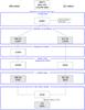 |
Fig. 1 Procedure for the generation of the working samples. From top to bottom, the number of stars in the samples decreases while the quality of the individual physical parameters increases. The left side shows the samples according to the MB method, and the right side with EC. |
In a first step, the available IPHAS initial data release (IDR; González-Solares et al. 2008), combined with our Hβ index, allowed us to detect and reject 1073 emission line stars. Then each approach to compute the physical parameters (i.e., MB and EC) required its own strategy. We created two different working samples: the first, hereafter MB-S1, with the 12 957 stars with Teff> 7000 K and SPP from the MB method, and the second, hereafter EC-S1, with 11 524 B0–A9 stars, with SPP derived using the EC method. Following the MB strategy, we considered as outliers the stars that lie 5σ outside the MB atmospheric grid during the 3D fit, taking into account the photometric errors in [ c1 ] − [ m1 ] − Hβ. We also removed stars with doubtful classification between photometric regions using Nside and Nreg flags. These flags, Nreg for the EC method and Nside for the MB method, indicate the probability for a star to belong to earlier or later photometric regions and were computed through Monte Carlo simulations (see Monguió et al. 2014, for details). Coherence with 2MASS data allowed us to reject some stars that cannot be allocated reliably to either early (B0-B9) or late (A3-A9) types. The two resulting “clean” samples contain 9781 (for MB-S2) and 9622 stars (for EC-S2). A new subset was built containing the stars that simultaneously belong to the young population following both methods. This was done by checking the coherence between the two sets of physical parameters. This cleanest sample contains 8328 stars and is named CS-MB or CS-EC depending on whether their physical parameters were computed using the MB or EC method (see Fig. 1). This sample contains stars with more accurate SPP data, but has fewer statistics owing to the lack of stars rejected during the cleaning process. From now on we will distinguish between the subsamples containing the stars in the inner sky area (in suffix), from those where the stars located in the outer sky area are added (all suffix). Whereas the first subsample reaches fainter limiting magnitude, the second contains more stars but is complete up to a brighter limiting magnitude. In Table 1 we give the number of stars for each of the subsamples.
Two sample KS test results of the comparison between solar luminosity function and luminosity function at different distances ranges.
Since we wanted to derive how the stellar density varies with the galactocentric distance, we needed to ensure that the features observed are due to a physical and real overdensity and not to observational or selection biases. To account for this, we created distance complete samples by selecting ranges of absolute magnitude, that ensured us distance completeness up to a given heliocentric distance. For each sample we estimated 1) the maximum visual limiting magnitude Vlim; 2) the magnitude at which some stars were saturated Vsat; and 3) the maximum and minimum visual interstellar absorption at a given distance. The Vlim for each of the samples, assuming a 90% completeness, was estimated by computing the mean of the magnitudes at the peak star counts in a magnitude histogram and its two adjacent bins, before and after the peak, weighted by the number of stars in each bin. In Monguió et al. (2013) we checked that this estimate is adequate by comparing the V magnitude distribution of the stars with all the available photometric indexes, and with the distribution observed for stars measured in V that reached a significant fainter limiting magnitude. To ensure an adequate range before and after the Perseus arm in the anticenter direction, we selected samples complete up to 3 kpc from the Sun. The maximum interstellar absorption at 3 kpc was estimated from AVmax(3 kpc) =  . This value was then used to compute the limit in the intrinsic star brightness: MVlim(3 kpc) = Vlim − AVmax(3 kpc) − 5log (3 kpc) + 5. In addition, stars brighter than Vsat = 11m may suffer from saturation problems (Monguió et al. 2013). Thus, we estimated and set a completeness limit in the absolute brightness – named MVlim(1.2 kpc) – for the closest distance, imposed to be 1.2 kpc, using both Vsat and the interstellar absorption at this distance. Following this strategy, that is, by selecting the stars with the absolute magnitude inside the computed range, all the resulting samples were converted to distance complete samples in the distance range between 1.2 and 3 kpc. Table 1 shows all the values used to generate each sample together with the number of stars included in each of them. Figure 2 shows an example of the apparent visual magnitude range needed to cover the distance range [1.2, 3] kpc for a star with a fixed absolute magnitude. As an example, this figure shows the limits on apparent visual magnitude assumed for the MB-S1, MB-S2, and CS-MB samples. We can see how these samples have complete populations inside the heliocentric distance range selected.
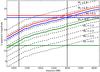 |
Fig. 2 Observed apparent magnitude for different absolute magnitude stars located at different distances. We have assumed an absorption of |


Finally, we checked that the distribution of effective temperature and spectral type included in each of our samples do not change as a function of distance within the [1.2, 3] kpc range. Several two-sample Kolmogorov-Smirnov (KS) tests were done comparing the luminosity function at different distances with the distribution at the solar neighborhood (obtained in Sect. 4.2, see Fig. 3). In all the cases, the KS tests are consistent with the assumption that the underlying luminosity functions arise from the same distribution (see Table 2). We observed that only for the farthest subsamples of MB-S1 and MB-S2 we do have small values of the p-values, but not enough to reject the null hypothesis at 0.01 level.
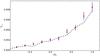 |
Fig. 3 Surface density at the Sun’s position for 0.2mMV bins, using both Vlim = 6m (in red) and |
Looking at Table 1 we see that the samples considering all the anticenter observed sky area, as the outer area has a brighter limiting magnitude, have a very narrow range in absolute magnitude, which means that the final number of stars in those samples is not high enough to undertake the study of the stellar overdensity induced by the Perseus arm with good statistical significance (Sect. 4).
4. Radial density distribution
The surface density was chosen over volume density to be the best parameter with which to trace the stellar distribution considering the information available, that is, a set of distance complete samples inside a solid angle of 8◦2 or 16◦2 in the anticenter direction (Sect. 3). This is a better choice since it gives an estimate of the total disk mass at a given distance, also taking into account the change in the mid-plane due to the warp, assuming that the disk scale height varies slowly with distance. All the factors taken into account in the derivation of this parameter from the data are described in Sect. 4.1. The radial bin size used to derive the galactocentric variation of this parameter was computed using the method proposed by Knuth (2006). As stated by the author, this method is optimized to find substructure in the data1. The radial scale length of the Galactic disk in the anticenter direction and the possible overdensity associated with Perseus were obtained by fitting an exponential function to the working samples described in Table 1. Initially, the two parameters of this function were fitted: the radial scale length (hR) and the surface density in the solar neighborhood (Σ⊙) of the population represented by these working samples. The fit highly depends on the zero point of the distribution Σ⊙. Thus, to substantially increase both the range in distance covered and the significance of the fit, we decided to derive this parameter independently using a local sample (see Sect. 4.2). Then these values were used in Sect. 4.3 to do the fits, where the departure of the exponential surface density distribution and the existence of possible maxima are discussed in terms of the location and existence of the overdensity associated with the Perseus spiral arm.
4.1. The computation of the stellar surface density
To derive the stellar surface density we included the sky area surveyed, the effect of the scale height of the underlying thin disk population being considered, as well as the presence of the Galactic warp. The surface density for each distance bin was computed as 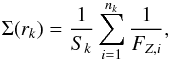 (1)where nk is the number of stars in a given radial bin k; Sk is the disk projected surface for that radial bin computed from the Galactic latitude ℓ covered, the mean distance to the Sun rk of the bin, and the distance width size of the bin in parsecs; FZ,i is a correction factor for each star that takes into account the fact that our observed solid angle does not cover the full vertical cylinder. This factor is assumed to depend on the vertical density distribution, modeled as sech2(z/hz) (van der Kruit & Searle 1981), with hz being the scale height of the disk. As is known, hz depends on the age of the population. Here, as an approximation, we model it as depending on the visual absolute magnitude of the star. Values for hz are not well determined, whereas Reed (2000) gave hz = 25–65 pc for OB-type stars (mainly O-B2), and Maíz-Apellániz (2001) obtained hz = 34.2 ± 2.5 pc for a sample of O-B5 stars. More recently, Kong & Zhu (2008), using Hipparcos data, estimated values around hz = 103.1 ± 3.0 pc for the full range of OB stars. Czekaj et al. (2014) adopted hz = 130 pc for stars with ages younger than 0.15 Gyr whereas values up to 260 pc were assumed for stars with ages between 0.15 and 1 Gyr. These simulations provide age ranges around 50 ± 20 Myr for B5-type stars (Teff ~ 15 000 K), while age ranges of 500 ± 200 Myr are obtained for A5-type stars (Teff ~ 8000 K). Taking into account these estimations, we adopted the relation hz(pc) = 36.8·MV + 130.9, which is equivalent to assuming 100 pc for B5-type stars and 200 pc for an A5-type star. It must be taken into account that a different relation between the scale height and the intrinsic brightness would change the zero point of the stellar density distribution, and thus the corresponding surface density at the Sun’s position Σ⊙. The FZ,i factor also takes into account the vertical range (zmin,i,zmax,i) covered at each galactocentric distance. Keeping this in mind, this factor is computed following
 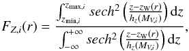 (2)where we also considered the position of the warp (zW(r)). From observational data (2MASS and HI data) Momany et al. (2006) obtained bW ~ −0.5° at ℓ = 180°, so we can assume that at different distances the zW, where the star density of the disk is maximum, can be computed as zW = rtanbW.
4.2. Surface density in the solar neighborhood
We used the Hauck & Mermilliod (1998) catalog of Strömgren photometry to compute the surface density at the Sun’s position for young stars. This process was done following the same methodology as we used for the anticenter stars, that is, the same computation of SPP, and the same process used to clean the samples (Sects. 2 and 3). First we checked the completeness of the Hauck & Mermilliod (1998) catalog in terms of the visual apparent magnitude. For that, we cross-matched this catalog with the Hipparcos catalog (ESA 1997). We verified that the completeness is above 95% up to 65 for OB stars. Strömgren photometric data allowed us to compute their physical parameters, selecting only those with Teff> 7000 K for MB, and B0–A9 for EC. To mimic the samples in the anticenter we selected the same MV ranges, and computed the distance limit for which we can ensure completeness (assuming in this case AV = 0): rlim = 10(Vlim − MVmax + 5)/5. We repeated the computations using Vlim = 6m and  and obtained very similar results. We considered the effect of the warp to be negligible in the solar neighborhood. We also checked that different values for the distance of the Sun above the Galactic plane gave results within the error bars: z⊙ = 15 pc from Robin et al. (2003) and z⊙ = 26 pc from Majaess et al. (2009). We used the same dependence of the scale height function on absolute magnitude as for the density in the anticenter direction (Sect. 4.1). In this case, the limits in z follow the surface of an sphere around the Sun’s position,
  , and the projected surface density is then easily modeled as
  . The obtained distribution for different magnitudes ranges of 02 is plotted in Fig. 3. For comparison, the values resulting from model B of the new Besançon Galaxy Model (Czekaj et al. 2014) are overplotted. These values were derived fitting the model to the full sky Tycho catalogue. In Fig. 3 we observe that the distribution is very similar in the whole range of absolute magnitudes, thus confirming the robustness of the derivation of the local surface density for the young population, i.e., the zero point of our exponential fit to the anticenter data. When we used the MV limits established for our samples (see Table 1), the values for the local surface density obtained were (3.25 ± 0.13) × 10-2 for MB-S1in and MB-S2in, (1.70 ± 0.07) × 10-2 for CS-MBin, (3.49 ± 0.12) × 10-2 for EC-S1in and EC-S2in, and (1.41 ± 0.06) × 10-2⋆/pc2 for CS-ECin. Their errors were computed as
 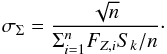 (3)
(3)
 |
Fig. 4 Radial variation of the stellar surface density for the MB (top) and EC (bottom) samples in blue. Vertical red lines show the 1.2 and 3 kpc completeness limits. The exponential fit is plotted in magenta, with the hR and Σ⊙ parameters expressed in pc and ⋆/pc2, respectively. Blue dots joined with solid lines are the ones used for the fit, since it is the region where completeness is ensured. |
4.3. The radial scale length and the detection of the Perseus arm
The radial surface density distribution was computed for all the samples and an exponential function was fitted to each of them by adopting the zero point values for the local surface density obtained in the previous section. The radial scale length of the Galactic disk in the anticenter direction is presented in Fig. 4. The scale lengths obtained for the fits using MB distances (Fig. 4, top panel) are in the range hR ~ [ 3.5−4.3 ] kpc. More importantly, we can clearly recognize the overdensity associated with the Perseus arm at around 1.6 kpc (depending slightly on the sample), within the distance range at which the samples are complete, that is, between 1.2 and 3 kpc from the Sun. The decline after 3 kpc is produced by the limiting magnitude of our samples, since we carefully checked that the completeness is only ensured up to this distance. The results for the EC method are presented in the bottom panels of Fig. 4. As discussed in Sect. 2, the photometric distances derived from this method are clearly biased, in the sense that EC distances can be 20% shorter than the MB distances, the latter being more congruent with Hipparcos parallaxes (the detailed comparison is given in Monguió et al. 2014). As a consequence of this bias, the overdensity bump associated with the Perseus arm is also present, but closer to us and overlapping with the short distance limit at 1.2 kpc imposed to avoid saturation effects from bright stars. Some attempts were made to fit the points beyond the arm, but the results obtained for the radial scale length are unrealistic (hR = [1.7, 1.9] kpc). For the samples using all the sky area, the number of stars in the range [1.2–3] kpc was too low, since the limiting magnitude was too bright, and the fainter stars included in the samples have MV = 0.2,–0.2, i.e., B7-B8.5 stars (see Table 1). Thus, the features related to the overdensity, although present, were less statistically significant than for the in samples.
The next step was to re-compute the exponential fitting, avoiding the points close to the peak detected, that is between 1.4 and 2.0 kpc (see Fig. 5). In this fit, a slight decrease of the radial scale length until hR = 2.9 ± 0.1/0.2 kpc for both MB-S1 and MB-S2 samples is obtained. For the cleanest sample CS-MB we obtain a slightly larger value of hR = 3.5 ± 0.5 kpc (right panel of Fig. 5). In this case, the uncertainty is significantly larger since the working sample contains fewer stars. In addition, the stars in this sample have a brighter apparent limiting magnitude with respect to the previous ones, so their corresponding MV range is shifted to intrinsically brighter objects, i.e., it contains a slightly younger population on average. This result is congruent with recent data obtained from simulations such as those presented by Bird et al. (2013), showing that the radial scale length increases when the population considered is younger.
The three samples using MB distances show a clear peak around 1.6 kpc (Figs. 4 and 5). This overdensity is clearer for those samples having larger number of stars (MB-S1 and MB-S2, left and central panels). Although they have a more robust statistical detection, they also contain values that are less accurate for the SPP and some contamination from adjacent photometric regions could also be present (see Sect. 2). Thus we consider that it is the whole set of fits presented in the top rows of Figs. 4 and 5, using the three samples, that allows us to confirm the detection of the stellar overdensity associated with the Perseus spiral arm.
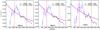 |
Fig. 5 Radial variation of the stellar surface density for the MB samples in blue. Vertical red lines show the 1.2 and 3 kpc completeness limits. Green dots show the points used for the exponential fit, avoiding those around the overdensity location. The exponential fit is plotted in magenta, with the hR and Σ⊙ parameters expressed in pc and ⋆/pc2, respectively. |
5. The Perseus arm overdensity
We performed χ2 tests for the different fits presented in the previous sections to quantitatively evaluate the significance of the detected Perseus arm overdensity. The number of stars observed ( , with k = 1,m) for each k distance bin between 1.2 and 3 kpc was compared with the distribution coming from the resulting exponential fit (see Fig. 6). To compare the model and the observations we use as a first approximation the number of corresponding stars at the central distance of each bin (
 ). The χ2 value was computed as
  (4)where was computed from the surface density obtained from the fitted expression
  and transformed to the number of stars per bin using:
  . The factor ⟨ FZ,i ⟩ is the average of FZ,i for all the stars in the bin previously used to transform from observed nk to observed surface density Σ(rk) (see Eq. (1)). Then, considering the degrees of freedom for each histogram (i.e., number of bins minus two, since hR and χ2 have been estimated), the test statistics were obtained. The hypothesis that the data come from a pure exponential distribution can be rejected at a 4–5σ confidence level for S1, S2, and CS samples for the inner sky area, so they clearly do not fit with an exponential. Looking at the plots, the overdensity at 1.6 kpc is the main reason for the deviation. The location of the peak of the distribution varies slightly for different samples, being at 1.5 kpc for MB-S1in, and 1.7 kpc for MB-S2in and CS-MBin. An error of 0.2 kpc (the bin width) has been adopted for this maximum overdensity.
On the other hand, when we rejected the points between 1.4 and 2.0 kpc (where the overdensity is detected) and repeat the fit, we obtained p-values from the χ2 test of 0.44, 0.50, and 0.10 for the S1, S2, and CS samples (those in Fig. 5). In other words, when we did not take into account the bins located close to the arm the distributions were fully compatible with an exponential fit.
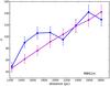 |
Fig. 6 Number of stars nk observed (in blue) and number of stars expected from the exponential fit |
We estimated the significance of the peak as  , where
  is the number of stars in the bins close to the arm (i.e., between 1.4 and 2.0 kpc) and
  is the expected number of stars from the exponential fit (where the arm bins were not used for the fit). The overdensity obtained for the MB-S1 and MB-S2 samples had a significance of 4.3σ. For CS-MB we obtained 3.0σ, a lower value due to the smaller number of stars included in the sample (see Table 3).
The amplitude of the arm A was estimated from the expression 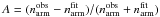 . The obtained values are presented in Table 3. For all samples we derive values in the range A=[0.12,0.14], well in agreement with recent determinations (see references of the density contrast of the Milky Way spiral arms discussed in Antoja et al. 2011). However, one should take into account the different methods used by these authors: Drimmel & Spergel (2001) obtained A = 0.14 from K-band surface brightness, while Benjamin et al. (2005) derived A = 0.13 from GLIMPSE data looking at the tangential points of the inner spiral arm. In external galaxies, Rix & Zaritsky (1995) gave values in the range 0.15 ≲ A ≲ 0.6, while Grosbøl et al. (2004) provided amplitudes for several galaxies, also from surface photometry in the K-band, reaching values up to A = 0.5, although they claimed that the amplitude varies as a function of radius. However, the same authors (Grosbøl & Patsis 2014) suggested that amplitudes measured in the K-band may be overestimated by a factor of 2 which bring the Perseus amplitude in agreement with measurements of external galaxies.
Number of stars between 1.4 and 2.0 kpc, and the expected value from the exponential when we do not take into account the arm bins.
 |
Fig. 7 2D extinction maps in (ℓ,b) at four different distances from the Sun, 1000, 1500, 2000, and 2500. AV is color coded, with a shift of 0.2m in the color scale between consecutive plots. |
6. The Perseus arm dust layer
Since both individual photometric distances and visual interstellar absorptions (AV) are available for a large sample of stars, a detailed 3D extinction map was created to discuss and quantify the possible existence of a dust layer related to the Perseus arm. In Sect 6.1 we present the maps and discuss some of the observed features, whereas in Sect. 6.2 the existence of a change in the differential absorption (dAV/dr) is discussed in order to determine if there is a high density interstellar region linked to the Perseus arm and, more importantly, to understand if this region is in front of or behind the stellar component of this arm.
6.1. Three-dimensional extinction map in the anticenter direction
The MB-S1 sample was used to create the 3D extinction map presented in Fig. 7. The number of stars in this sample allowed us to reach distances up to 2.5–3 kpc. The grid inside the 3D cone was constructed taking 20 pc steps in distance and 2.5 arcmin steps in both Galactic longitude and latitude. At each point of the grid, the absorption AV was computed as  (5)where N is the total number of stars in the sample and Δri is the distance between the ith star and the point of the grid. The σ value is the radius used for the Gaussian weight computed as σ = r·atan(α) with α = 0.25°. This method allowed us to obtain a grid with higher spatial resolution in nearby regions where we had more information, and less at further distances where information was poorer. We note that this method would introduce some bias at the edges of the grid. The lack of data outside the surveyed area can result in mean values of the AV(r,l,b) that are slightly biased towards the values present in the inner parts. We estimate that this bias should be present only in areas at angular distances less than about 0.5° (2σ) from the survey’s edges.
In Fig. 7 we plotted the AV values of the grid points placed at four distances and computed following Eq. (5). A first comparison can be done with the integrated extinction maps obtained by Froebrich et al. (2007), using 2MASS data (Fig. 8, top), and those recently derived by the Planck collaboration (2014; Fig. 8, bottom). As expected the same general trends are observed in these maps clearly identifying the same very low and very high extinction areas. Whereas both maps in Fig. 8 indicate the total dust integrated intensity towards a given line of sight, our 3D map is able to distinguish features at specific distances. Although our data avoids the presence of some of the biases thoroughly discussed in Froebrich et al. (2007), we note that it is not the goal of this paper to investigate the individual distribution of clouds or their sizes and mass distribution, which are discussed in that paper. In the Froebrich maps, for example, regions close to rich star clusters would be dominated by the colours of the cluster members; instead, the data presented here do not suffer from this bias. As an example of the future scientific exploitation of this 3D map we here comment on the distribution of interstellar medium around the supernova remnant (SNR) Simieis 147. This SNR has its geometrical center at (l,b) = (180.17, b = −1.81) with a diameter of about 180 arcmin (Green 2009). Its suggested distance ranges from 0.6 to 1.9 kpc (see Table 1 from Dinçel et al. 2015). For its related pulsar PSRJ0538+2817 Ng et al. (2007) estimated a distance of  kpc and Fesen et al. (1985) an absorption of AV = 0.76 ± 0.2 magnitudes. At the edge of our survey our 3D extinction map indicates a slightly higher absorption at larger distances (at about 2 kpc) and a more prominent absorption at the area surrounding the geometrical center proposed by Green (2009). As a second example we discuss the features visible around (ℓ,b) ~ (182.0,0.0) in the 1.5 kpc and 2 kpc maps. Rodríguez et al. (2006) found a molecular cloud in the anticenter direction associated with the two IRAS sources IRAS 05431+2629 at (ℓ,b) = (182.1, −1.1) and IRAS 05490+2658 at (ℓ,b) = (182.4, + 0.3). This last HII region was also found by Blitz et al. (1982) at (ℓ,b) = (182.36, + 0.19) through CO observations, and they give a distance of 2.1±0.7 kpc. We observed a weak but well-defined high mean density region at this distance. These are only examples of the potential interest of these maps, and it will be through future analysis that multivariate clustering techniques will be applied to our grid points to confirm and characterize the clumpy structures present in the cone defined by our anticenter survey.
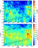 |
Fig. 8 Top: extinction map from Froebrich et al. (2007) based on 2MASS data. Bottom: thermal the dust radiance ℛ map (or dust integrated intensity) from Planck data (Planck Collaboration XI 2014). |
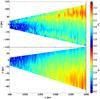 |
Fig. 9 Top: 2D extinction map in (x,y), where stars for all z were used for the average. Bottom: 2D extinction map in (x,z), where absorption for the stars at all y were averaged. AV is color coded. |
Recently, Chen et al. (2014) obtained a 3D extinction map with a spatial resolution of 3–9 arcmin by using multiband photometry. In this study individual distances are not available, so to break the degeneracy between the intrinsic stellar colours and the amounts of extinction the authors relied on the combination of optical and near-infrared photometric data. Our maps presented in Fig. 7, although with less spatial resolution, are based on individual distances with accuracies at about 10–20% (Monguió et al. 2014). We understand that both studies provide complementary information for future analysis.
As a final example, in Fig. 9 we show the 2D extinction map projected on the cartesian coordinates (x,y) and (x,z) planes where the absorptions at different z and y were averaged. The x-axis is positive toward the anticenter, y in the direction of Galactic rotation, while z toward the north Galactic pole. These maps allowed us to analyze the change of extinction with distance. We observed that larger extinction regions were placed at lower Galactic longitudes and below the Galactic plane. This large-scale dust distribution is discussed in the next section in the context of the presence of the Perseus spiral arm.
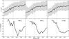 |
Fig. 10 Top: running median of the visual absorption vs. heliocentric distance distribution obtained from the three different samples MB-S1 (left), MB-S2 (middle), and CS (right). The gray area indicates the error of the median computed as |

6.2. Absorption distribution as a function of distance
Here, to reinforce the detection of the stellar overdensity of the Perseus arm presented in Sect. 5, we present in Fig. 10 (top) the median distribution of the visual absorption as a function of distance. We can clearly appreciate a change in the slope at the same position where we detected the stellar overdensity of Perseus, which is at about 1.6 kpc. This change is better identified by plotting its derivative as a function of distance (dAV/dr) (see Fig. 10, bottom). We observed that this derivative presents two different well-defined values, a high value of about 0.8–1.0 mag/kpc in front of the stellar arm, and a significantly lower value of about 0.2–0.4 mag/kpc behind the arm. We would expect, for constant absorption, a flat distribution of the dAV/dr, while the presence of a cloud or dust layer would be translated into a bump in the dAV/dr distribution. We can see this change in slope in all the directions, suggesting the presence of a dust layer just before the position of the density peak associated with the Perseus arm.
As described by Roberts (1969), the star formation induced by the shock in a stellar density wave scenario would produce an azimuthal age sequence across the spiral arms. However, as a first attempt, we analyze the dust distribution (i.e., interstellar extinction) in this context. The presence of the dust lane at the inner side of the stellar overdensity indicates a compression or shock in the gas associated with the spiral arm (although the strict coincidence of a shock and a lane is not obligatory; Gittins & Clarke 2004). From this we can use our first analysis of the 3D extinction map to establish a limit on the co-rotation (CR) radius in the Milky Way Galactic disk (Roberts 1972). A discussion on the optical tracers of spiral wave resonances in external galaxies can be found in Elmegreen et al. (1992). Puerari & Dottori (1997) provided a good sketch of the Z-trailing spatial arms configuration expected for the Milky Way (see their Fig. 1). Figure 10 (right) suggests that the dust layer is just in front of the Perseus arm so the CR radius of the spiral pattern (if a density wave scenario is assumed) is outside the location of Perseus in the anticenter direction: RCR> 10.2 kpc (assuming R⊙ = 8.5 kpc). This result is closely in agreement with the position of the CR radius suggested by Antoja et al. (2011), who, from a kinematic analysis of the moving groups in the solar neighborhood, proposed an angular velocity of the perturbation (Ωp) of about 16–20 km s-1 kpc-1, so with a galactocentric co-rotation radius at about RCR = 11–14 kpc.
7. Summary and conclusions
In Monguió et al. (2013, 2014) we published a deep Strömgren photometric survey and a new strategy for the derivation of stellar physical parameters for the young stellar population in the anticenter direction. Here we used these data to derive samples of intermediate young stars, complete within the distance range between 1.2 and 3.0 kpc from the Sun. We computed the surface density distribution in the anticenter direction by assuming a vertical density distribution of the disk, taking into account the surveyed area and the warp, so carefully defining correction functions for all the observational and physical effects. The same strategy was used to compute the surface density at the Sun’s position through Hauck & Mermilliod (1998) Strömgren data, obtaining 0.032 ± 0.001 ⋆/pc2 and 0.017 ± 0.001 ⋆/ pc2 for stars in the MV = [ −0.9,1.2 ] and MV = [ −0.9,0.8 ] ranges, respectively. The exponential functions fitted to the computed stellar surface density revealed a clear star overdensity at around 1.6 ± 0.2 kpc that we associate with the presence of the Perseus spiral arm. The obtained distance is slightly closer than the 2.0 kpc recently obtained by Reid et al. (2014) who traced the arm using star forming regions. The fits we performed avoiding the bins close to the arm location, allowed us to derive the radial scale length of the Galactic disk young population, obtaining hR = 2.9 ± 0.1 kpc for B4–A1 stars, and hR = 3.5 ± 0.5 kpc for B4–A0 stars. The overdensity associated with the Perseus arm has been detected with a significance above 3σ in all cases, and above 4σ for the samples with larger statistics. Our results indicate that the star density contrast of the young population in Perseus is on the order of A = 0.12–0.14. This quantitative estimation of the spiral arm amplitude in the anticenter – derived here for the first time – should be understood as a contribution to the future derivation of the amplitude changes of the Milky Way spiral pattern as a function of galactocentric radius. So far, this radial change has only been clearly detected in external galaxies (e.g., Grosbøl et al. 2004).
Also very important, the distribution of visual interstellar absorption as a function of distance reveals the presence of a dust layer in front of the Perseus arm, which suggests that it is placed inside the co-rotation radius of the Milky Way spiral pattern. Our results locate the co-rotation radius at least two kiloparsecs outside the Sun’s position. This is the first time that the presence of the Perseus arm has been detected through individual star counts, and its presence is being supported by the dust distribution.
Acknowledgments
This work was supported by the MINECO (Spanish Ministry of Economy) – FEDER through grant AYA2009-14648-C02-01 and CONSOLIDER CSD2007-00050. M. Monguió was supported by a Predoctoral fellowship from the Spanish Ministry (BES-2008-002471 through ESP2006-13855-C02-01 project).
References
- Antoja, T., Figueras, F., Romero-Gómez, M., et al. 2011, MNRAS, 418, 1423 [NASA ADS] [CrossRef] [Google Scholar]
- Benjamin, R. A. 2008, in Massive Star Formation: Observations Confront Theory, eds. H. Beuther, H. Linz, & T. Henning, ASP Conf. Ser., 387, 375 [Google Scholar]
- Benjamin, R. A., Churchwell, E., Babler, B. L., et al. 2005, ApJ, 630, L149 [NASA ADS] [CrossRef] [Google Scholar]
- Bird, J. C., Kazantzidis, S., Weinberg, D. H., et al. 2013, ApJ, 773, 43 [NASA ADS] [CrossRef] [MathSciNet] [Google Scholar]
- Blitz, L., Fich, M., & Stark, A. A. 1982, ApJS, 49, 183 [NASA ADS] [CrossRef] [Google Scholar]
- Chen, B.-Q., Liu, X.-W., Yuan, H.-B., et al. 2014, MNRAS, 443, 1192 [NASA ADS] [CrossRef] [Google Scholar]
- Czekaj, M. A., Robin, A. C., Figueras, F., Luri, X., & Haywood, M. 2014, A&A, 564, A102 [NASA ADS] [CrossRef] [EDP Sciences] [Google Scholar]
- Dame, T. M., Hartmann, D., & Thaddeus, P. 2001, ApJ, 547, 792 [NASA ADS] [CrossRef] [Google Scholar]
- Dinçel, B., Neuhäuser, R., Yerli, S. K., et al. 2015, MNRAS, 448, 3196 [NASA ADS] [CrossRef] [Google Scholar]
- Drimmel, R. 2000, A&A, 358, L13 [NASA ADS] [Google Scholar]
- Drimmel, R., & Spergel, D. N. 2001, ApJ, 556, 181 [NASA ADS] [CrossRef] [Google Scholar]
- Elmegreen, B. G., Elmegreen, D. M., & Montenegro, L. 1992, ApJS, 79, 37 [NASA ADS] [CrossRef] [Google Scholar]
- Fesen, R. A., Blair, W. P., & Kirshner, R. P. 1985, ApJ, 292, 29 [NASA ADS] [CrossRef] [Google Scholar]
- Foster, T. J., & Brunt, C. M. 2014, AJ, submitted [arXiv:1405.7003] [Google Scholar]
- Froebrich, D., Murphy, G. C., Smith, M. D., Walsh, J., & Del Burgo, C. 2007, MNRAS, 378, 1447 [NASA ADS] [CrossRef] [Google Scholar]
- Gittins, D. M., & Clarke, C. J. 2004, MNRAS, 349, 909 [NASA ADS] [CrossRef] [Google Scholar]
- González-Solares, E. A., Walton, N. A., Greimel, R., et al. 2008, MNRAS, 388, 89 [NASA ADS] [CrossRef] [Google Scholar]
- Grand, R. J. J., Kawata, D., & Cropper, M. 2012, MNRAS, 421, 1529 [CrossRef] [Google Scholar]
- Green, D. A. 2009, VizieR Online Data Catalog: VII/253 [Google Scholar]
- Grosbøl, P., & Patsis, P. A. 2014, in ASP Conf. Ser. 480, eds. M. S. Seigar, & P. Treuthardt, 117 [Google Scholar]
- Grosbøl, P., Patsis, P. A., & Pompei, E. 2004, A&A, 423, 849 [NASA ADS] [CrossRef] [EDP Sciences] [Google Scholar]
- Hauck, B., & Mermilliod, M. 1998, A&AS, 129, 431 [NASA ADS] [CrossRef] [EDP Sciences] [Google Scholar]
- Knuth, K. H. 2006, ArXiv e-prints [arXiv:physics/0605197] [Google Scholar]
- Kong, D.-L., & Zhu, Z. 2008, Chin. Astron. Astrophys., 32, 360 [NASA ADS] [CrossRef] [Google Scholar]
- Lin, C. C., & Shu, F. H. 1964, ApJ, 140, 646 [NASA ADS] [CrossRef] [MathSciNet] [Google Scholar]
- Lindblad, P. O. 1967, in Radio Astronomy and the Galactic System, ed. H. van Woerden, IAU Symp., 31, 143 [Google Scholar]
- Maíz-Apellániz, J. 2001, AJ, 121, 2737 [Google Scholar]
- Majaess, D. J., Turner, D. G., & Lane, D. J. 2009, MNRAS, 398, 263 [NASA ADS] [CrossRef] [Google Scholar]
- Momany, Y., Zaggia, S., Gilmore, G., et al. 2006, A&A, 451, 515 [NASA ADS] [CrossRef] [EDP Sciences] [Google Scholar]
- Monguió, M., Figueras, F., & Grosbøl, P. 2013, A&A, 549, A78 [NASA ADS] [CrossRef] [EDP Sciences] [Google Scholar]
- Monguió, M., Figueras, F., & Grosbøl, P. 2014, A&A, 568, A119 [NASA ADS] [CrossRef] [EDP Sciences] [Google Scholar]
- Ng, C.-Y., Romani, R. W., Brisken, W. F., Chatterjee, S., & Kramer, M. 2007, ApJ, 654, 487 [NASA ADS] [CrossRef] [Google Scholar]
- Planck Collaboration XI. 2014, A&A, 571, A11 [NASA ADS] [CrossRef] [EDP Sciences] [Google Scholar]
- Puerari, I., & Dottori, H. 1997, ApJ, 476, L73 [NASA ADS] [CrossRef] [Google Scholar]
- Reed, B. C. 2000, AJ, 120, 314 [NASA ADS] [CrossRef] [Google Scholar]
- Reid, M. J., Menten, K. M., Brunthaler, A., et al. 2014, ApJ, 783, 130 [Google Scholar]
- Rix, H.-W., & Zaritsky, D. 1995, ApJ, 447, 82 [NASA ADS] [CrossRef] [Google Scholar]
- Roberts, W. W. 1969, ApJ, 158, 123 [NASA ADS] [CrossRef] [Google Scholar]
- Roberts, Jr., W. W. 1972, ApJ, 173, 259 [NASA ADS] [CrossRef] [Google Scholar]
- Robin, A. C., Reylé, C., Derrière, S., & Picaud, S. 2003, A&A, 409, 523 [NASA ADS] [CrossRef] [EDP Sciences] [Google Scholar]
- Rodríguez, M. I., Allen, R. J., Loinard, L., & Wiklind, T. 2006, ApJ, 652, 1230 [NASA ADS] [CrossRef] [Google Scholar]
- Romero-Gómez, M., Athanassoula, E., Masdemont, J. J., & García-Gómez, C. 2007, A&A, 472, 63 [NASA ADS] [CrossRef] [EDP Sciences] [Google Scholar]
- Russeil, D. 2003, A&A, 397, 133 [NASA ADS] [CrossRef] [EDP Sciences] [Google Scholar]
- Strömgren, B. 1966, ARA&A, 4, 433 [NASA ADS] [CrossRef] [Google Scholar]
- Vallée, J. P. 2014, ApJS, 215 [Google Scholar]
- van der Kruit, P. C., & Searle, L. 1981, A&A, 95, 105 [NASA ADS] [Google Scholar]
- Vázquez, R. A., May, J., Carraro, G., et al. 2008, ApJ, 672, 930 [NASA ADS] [CrossRef] [Google Scholar]
- Xu, Y., Reid, M. J., Zheng, X. W., & Menten, K. M. 2006, Science, 311, 54 [NASA ADS] [CrossRef] [PubMed] [Google Scholar]
All Tables
Two sample KS test results of the comparison between solar luminosity function and luminosity function at different distances ranges.
Number of stars between 1.4 and 2.0 kpc, and the expected value from the exponential when we do not take into account the arm bins.
All Figures
|
Fig. 1 Procedure for the generation of the working samples. From top to bottom, the number of stars in the samples decreases while the quality of the individual physical parameters increases. The left side shows the samples according to the MB method, and the right side with EC. |
| In the text | |
|
Fig. 2 Observed apparent magnitude for different absolute magnitude stars located at different distances. We have assumed an absorption of |
| In the text | |
|
Fig. 3 Surface density at the Sun’s position for 0.2mMV bins, using both Vlim = 6m (in red) and |
| In the text | |
|
Fig. 4 Radial variation of the stellar surface density for the MB (top) and EC (bottom) samples in blue. Vertical red lines show the 1.2 and 3 kpc completeness limits. The exponential fit is plotted in magenta, with the hR and Σ⊙ parameters expressed in pc and ⋆/pc2, respectively. Blue dots joined with solid lines are the ones used for the fit, since it is the region where completeness is ensured. |
| In the text | |
|
Fig. 5 Radial variation of the stellar surface density for the MB samples in blue. Vertical red lines show the 1.2 and 3 kpc completeness limits. Green dots show the points used for the exponential fit, avoiding those around the overdensity location. The exponential fit is plotted in magenta, with the hR and Σ⊙ parameters expressed in pc and ⋆/pc2, respectively. |
| In the text | |
|
Fig. 6 Number of stars nk observed (in blue) and number of stars expected from the exponential fit |
| In the text | |
|
Fig. 7 2D extinction maps in (ℓ,b) at four different distances from the Sun, 1000, 1500, 2000, and 2500. AV is color coded, with a shift of 0.2m in the color scale between consecutive plots. |
| In the text | |
|
Fig. 8 Top: extinction map from Froebrich et al. (2007) based on 2MASS data. Bottom: thermal the dust radiance ℛ map (or dust integrated intensity) from Planck data (Planck Collaboration XI 2014). |
| In the text | |
|
Fig. 9 Top: 2D extinction map in (x,y), where stars for all z were used for the average. Bottom: 2D extinction map in (x,z), where absorption for the stars at all y were averaged. AV is color coded. |
| In the text | |
|
Fig. 10 Top: running median of the visual absorption vs. heliocentric distance distribution obtained from the three different samples MB-S1 (left), MB-S2 (middle), and CS (right). The gray area indicates the error of the median computed as |
| In the text | |
Current usage metrics show cumulative count of Article Views (full-text article views including HTML views, PDF and ePub downloads, according to the available data) and Abstracts Views on Vision4Press platform.
Data correspond to usage on the plateform after 2015. The current usage metrics is available 48-96 hours after online publication and is updated daily on week days.
Initial download of the metrics may take a while.