| Issue |
A&A
Volume 577, May 2015
|
|
|---|---|---|
| Article Number | A21 | |
| Number of page(s) | 22 | |
| Section | Catalogs and data | |
| DOI | https://doi.org/10.1051/0004-6361/201322518 | |
| Published online | 24 April 2015 | |
VIMOS integral field spectroscopy of blue compact galaxies
I. Morphological properties, diagnostic emission-line ratios, and kinematics⋆,⋆⋆
1
Institut für Astrophysik, Georg-August-Universität,
Friedrich-Hund-Platz 1,
37077
Göttingen, Germany
e-mail: luzma@astro.physik.uni-goettingen.de
2
Instituto de Astrofísica de Canarias, 38200, La
Laguna, Tenerife, Spain
3
Departamento de Astrofísica, Universidad de la
Laguna, 38205,
La Laguna, Tenerife,
Spain
e-mail: nicola.caon@iac.es
4
Leibniz-Institut für Astrophysik Potsdam (AIP),
An der Sternwarte 16,
14482
Potsdam,
Germany
e-mail: pweilbacher@aip.de
Received:
21
August
2013
Accepted:
5
January
2015
Context. Blue compact galaxies (BCG) are gas-rich, low-luminosity, low-metallicity systems that undergo a violent burst of star formation. These galaxies offer us a unique opportunity to investigate collective star formation and its effects on galaxy evolution in a relatively simple environment. Spatially resolved spectrophotometric studies of BCGs are essential for a better understanding of the role of starburst-driven feedback processes on the kinematical and chemical evolution of low-mass galaxies near and far.
Aims. We carry out an integral field spectroscopic study of a sample of BCGs, with the aim of probing the morphology, kinematics, dust extinction, and excitation mechanisms of their warm interstellar medium.
Methods. Eight BCGs were observed with the VIMOS integral field unit at the Very Large Telescope using blue and orange grisms in high-resolution mode. At a spatial sampling of 0''̣67 per spaxel, we covered about 30″ × 30″ on the sky, with a wavelength range of 4150...7400 Å. Emission lines were fitted with a single Gaussian profile to measure their wavelength, flux, and width. From these data we built two-dimensional maps of the continuum and the most prominent emission-lines, as well as diagnostic line ratios, extinction, and kinematic maps.
Results. An atlas has been produced with the following: emission-line fluxes and continuum emission; ionization, interstellar extinction, and electron density maps from line ratios; velocity and velocity dispersion fields. From integrated spectroscopy, it includes tables of the extinction corrected line fluxes and equivalent widths, diagnostic-line ratios, physical parameters, and the abundances for the brightest star-forming knots and for the whole galaxy.
Key words: galaxies: dwarf / galaxies: starburst / galaxies: kinematics and dynamics
Based on observations made with ESO Telescopes at the Paranal Observatory under program ID 079.B-0445.
The reduced datacubes and their error maps (FITS files) are only available at the CDS via anonymous ftp to cdsarc.u-strasbg.fr (130.79.128.5) or via http://cdsarc.u-strasbg.fr/viz-bin/qcat?J/A+A/577/A21
© ESO, 2015
1. Introduction
Blue compact galaxies (BCGs) are gas-rich, low-luminosity (MB ranges from −12 to −21) systems experiencing intense ongoing star formation. They are characterized by their H ii region spectra (Thuan & Martin 1981), low metallicities (7.1 ≤ 12 + log (O / H) ≤ 8.4; Kunth & Östlin 2000), and intense star formation activity (rates ranging between 0.1 and 1 M⊙ yr-1; Fanelli et al. 1988; Hunter & Elmegreen 2004). In most of these galaxies, the gas consumption time scale is much shorter than the age of the Universe, which, together with their low metal content, initially led to the hypothesis that they could be truly young galaxies in the process of forming their first generation of stars (Kunth et al. 1988). Subsequent deep photometric studies (Loose & Thuan 1986; Papaderos et al. 1996; Cairós et al. 2001a,b; Gil de Paz et al. 2003) and Hubble Space Telescope (HST) color–magnitude diagrams (Schulte-Ladbeck et al. 1999, 2000, 2001; Aloisi et al. 2005, 2007) revealed that the vast majority of them have an underlying stellar population with ages of at least a few Gyr. In about two percent of the BCG galaxy population, however, an underlying population of stars has not been identified so far. These compact objects, with very low metallicities (12 + log (O / H) ≤ 7.65), are referred to as eXtremely Metal Deficient (XMD) galaxies, and they constitute the best local analogs to the distant subgalactic units from which larger galaxies are formed (Kunth & Östlin 2000). BCGs are paramount in extragalactic astronomy and observational cosmology research, because they hold key clues to understanding fundamental topics, such as galaxy formation and evolution and the star formation process.
Star-forming (SF) low-luminosity galaxies represent an unparalleled link to the early Universe, since in the well-accepted framework of a cold dark matter universe, structure formed hierarchically, with small scale objects (low-mass galaxies) collapsing first at relatively high redshifts. The un-evolved XMDs are the best local analogs of the “building blocks” in the early merger process (Kniazev et al. 2004), and their gas richness and metal deficiency make them excellent “laboratories” for constraining the parameters governing the primordial nucleosynthesis (Izotov et al. 1994).
The more luminous BCGs (or different subsamples of them) have been regarded as the local counterparts of SF galaxy populations at different redshifts, such as the faint blue galaxies (Cowie et al. 2001), luminous compact blue galaxies (Guzmán et al. 1997), Lyman-break galaxies (LBG, Grimes et al. 2009), or Lyman-α emitters (Mas-Hesse et al. 2003). Detailed analysis of nearby BCGs are essential to interpret the observations of these more distant SF galaxy populations, as their proximity allows for studies focused on their stellar populations, kinematics, and abundances with an accuracy and spatial resolution that cannot be achieved at higher redshifts (Cairós et al. 2009a,b, 2010).
Also, feedback from massive stars is believed to play a key role in the formation and evolution of galaxies (White & Rees 1978; Sommer-Larsen et al. 1999). In low-mass galaxies, their smaller gravitational potential can make the consequences of the feedback especially dramatic. Detailed studies of nearby BCGs are essential for understanding the feedback mechanism at higher redshifts and providing the input required for cosmological models.
A lot of work has been done in BCGs during the past two decades, but despite the large amount of effort invested, no conclusive answer has been reached so far for the most fundamental questions in the field, namely:
-
What are the mechanisms responsible for igniting the starburst in BCGs?
-
What is the evolutionary status of these galaxies? Are they (or some of them) truly young systems?
-
What is their star formation history?
Integral field spectroscopy (IFS) is the best way to approach BCG studies in a highly effective manner (Izotov et al. 2006a; García-Lorenzo et al. 2008; Vanzi et al. 2008; James et al. 2009; Cairós et al. 2009a,b, 2010). From only one integral field unit (IFU) frame, we can produce a series of broad-band images in a large number of filters, narrow-band images in a large set of bands, and can derive a large collection of observables from the spectrum (e.g., line indices, Wolf-Rayet features, etc.). Furthermore, we have all the information needed for every spatial resolution element, meaning that additional spatial constraints can be applied to restrict the typically degenerated population model solutions. For instance, the ages and star-formation history of each resolution element inside the same SF knot should be consistent. Such cross-checking helps avoid non-uniqueness in the model solutions.
Galaxy sample.
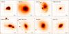 |
Fig. 1 Broad-band images of the galaxies of the sample. The field of view is 1′ × 1′, while the inner box marks the |

The work presented here is part of the IFS-BCG survey project, which aims to perform an exhaustive spectrophotometric investigation of a large sample of BCGs by means of IFS. The main scientific goals of this project include: i) disentangling and characterizing the different stellar populations in BCGs (e.g., constraining their ages, initial mass function and metallicity); ii) investigating the evolutionary status of the galaxies and constraining their star formation history; iii) probing the mechanism responsible for their actual burst of star formation; iv) analyzing the feedback effects between massive stars and the interstellar medium (ISM) in dwarf galaxies; v) investigating the recent suggestion that BCGs harbor active galactic nuclei (AGN) associated with intermediate-mass black holes; vi) providing an accurate dataset of photometric and spectroscopic parameters for a large sample of nearby SF dwarf galaxies, the essential template for understanding the results of the investigations at intermediate and high-z.
This is the fifth paper presenting results from our BGC-IFS survey. In Cairós et al. (2009a,b), we illustrated the full potential of this study by showing results for two representative BCGs, Mrk 409 and Mrk 1418, both observed with the Potsdam multi-aperture spectrophotometer (PMAS). A more detailed description of the project objectives, IFU observations, and reduction techniques, along with results for another eight objects observed with PMAS, was presented in Cairós et al. (2010). Finally, in Cairós et al. (2012), we reported results for five luminous BCDs observed with VIRUS-P, the prototype instrument for VIRUS (=Visible Integral-field Replicable Unit Spectrograph).
This paper is structured as follows. In Sect. 2 we introduce the sample and describe the observations, the data reduction process, and the method employed to derive the maps. In Sect. 3 we present the continuum and emission line intensity, emission line ratio, and velocity and velocity-dispersion maps. These results are discussed in Sect. 4 and summarized in Sect. 5.
2. The data
2.1. The galaxy sample
The IFS-BCG survey is a major program aimed at the study of the two-dimensional internal structure of a representative collection of BCG galaxies. The sample, which is made of about 40 objects, has been chosen so as to span the large interval in luminosities (MB ranges from −12 to −21), metallicities (7.1 ≤ 12 + log (O / H) ≤ 8.4), and morphologies (Cairós et al. 2001a) found among the galaxies classified as BCGs.
Here we present results for eight objects, which were observed working with the Visible Multi-Object Spectrograph (VIMOS; Le Fèvre et al. 2003) at the Very Large Telescope (VLT; ESO Paranal Observatory, Chile) at Unit Telescope 3 (Melipal) in the integral field unit mode. The basic data of the sample are listed in Table 1. The galaxies are located at distances between about 13 and 85.9 Mpc, which translates into angular sampling ranging from 63 to 416 pc arcsec-1. These objects span a wide range of morphologies (see Fig. 1), with three of them, namely Haro 11, Haro 15, and Tololo 1924-416, showing features of interactions. Interestingly, these three galaxies are also the most luminous in the sample, and they do not fit in the dwarf classification.
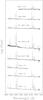 |
Fig. 2 Spectra of the galaxies of the sample in relative, logarithmic flux units. Telluric absorption was not corrected. |
Optical images of the galaxies are presented in Fig. 1. Spectra integrated over an aperture 10 pix (6.̋7) in radius, centered on the continuum peak at 5500 Å, and combined from the two wavelength ranges, are displayed in Fig. 2.
2.2. Observations
We observed in Visitor mode, during the nights August 19–21, 2007. With the blue grism (HR-blue), we covered a wavelength range of 4150–6200 Å with a dispersion of 0.51 Å pix-1, and with the orange (HR-orange), we covered the interval 5250–7400 Å with a dispersion of 0.60 Å pix-1. In this mode, the spatial sampling of the IFU is  , covering 27″ × 27″ on the sky. For a detailed description of the instrument and data reduction, see Le Fèvre et al. (2003) and Zanichelli et al. (2005).
The observing strategy was dictated by the VIMOS instrument characteristics. High flexures made it mandatory at the time to take calibration frames at short time intervals. The observing blocks (OBs) were usually composed of three dithered exposures of 720 s on target (with a few targets observed for 900 s per exposure) and one off-target pointing in order to allow sky subtraction. The three-point dither pattern used steps of a small multiple of the spaxel size to cover regions with bad or dead spaxels. The sky exposures were as long as the ontarget exposures. For most of the galaxies, the total observing time was split into two OBs. Calibrations exposures (lamp flats and arcs) are also included in the same OBs. The spectrophotometric standard EG274 was observed for flux calibration.
Weather conditions were generally good, except for strong winds during the third night that forced us to observe backup objects in a sky position away from the wind. The range in seeing (from the values given by the Paranal seeing monitor available from the FITS headers) and airmass for the exposures are given in Table 2.
Log of the observations.
2.3. Data reduction
The first part of the data reduction was performed using the ESO VIMOS pipeline (version 2.1.111) via the graphical user interface Gasgano. Gasgano allows us to comfortably organize calibration and science frames, and to start the pipeline tasks. Each VIMOS quadrant is an independent spectrograph, characterized by its own parameters. Therefore, data for each quadrant are handled separately by the pipeline.
The master bias frames were created by running the vmbias recipe. After that, vmifucalib produces the spectral extraction mask, the wavelength calibration, and a fiber-to-fiber relative transmission correction. Finally, vmifustandard creates the flux response curves from the spectrophotometric standard star spectrum. The products of these three tasks are then introduced in the recipe vmifuscience that reduces and extracts the final spectra, creating row-stacked, flux-calibrated spectra files for each quadrant of each exposure, sampled at 0.54 Å pix-1 and 0.62 Å pix-1 for blue and orange grisms, respectively. These data need to be sky-subtracted, and multiple, dithered exposures of the same target have to be combined for improved signal-to-noise (S/N).
The spectra are cut to only include wavelength ranges common to all fibers of all quadrants. Operating per quadrant, a sky spectrum is created from the sky exposure closest in time: the spectra with the lowest integrated average value are combined using minmax rejection to exclude cosmic rays and fibers with low values. Typically, the 200 lowest spectra are averaged, after rejecting the 50 highest and lowest pixels in each wavelength bin. The sky spectrum therefore effectively consists of the mean of 100 spectra. To subtract this sky spectrum from the object data of the same quadrant, the flux and wavelength of one of the brightest sky emission lines is measured in the sky spectrum and each object spectrum. (For the blue exposures, the line at 5577 Å works well, and for the orange exposures the line at 6864 Å gives the best compromise across the wavelength range.) We subtract the scaled and shifted sky spectrum2. This does not work optimally for all features of the sky background, since most components vary quickly with time, but residuals are generally located in spectral regions where we do not measure object features.
Before combining the exposures, the row-stacked spectra are converted into datacubes, using a fiber-position table. The exposure combination is done as image combination for each wavelength plane: the monochromatic images are shifted to take the dither pattern used during the observations into account. Shifts between exposures are visually optimized per object (using the plane of the brightest emission line in each range, i.e., [O iii] λ5007 in the blue exposures and Hα for the orange data), because the actual dither positions do not always agree with the expected offsets between exposures. The images are combined, using a sigma-clipping algorithm to reject most cosmic ray hits. Known bad spaxels are masked during this procedure. This procedure is carried out for the sky-subtracted files and files that still contain the sky emission. The bright sky emission lines in the exposures with sky were used for cross-checks of the velocity zeropoint of each spaxel. This way it was discovered that wavelength region around the [O iii] λ5007 line (the red end of the exposures with the blue grism) is not constrained well enough by arc lines in the wavelength calibration exposures, so can give small offsets (a few km s-1) depending on the spatial position within the IFU. The middle of the orange exposures are calibrated much better, so the Hα line should be used for velocity determination where possible.
We made a first assessment of the accuracy of the flux calibration by comparing the integrated fluxes, within the same central area, of the He iλ5876 line in the orange and blue spectra. The mean value of F(He i)orange/F(He i)blue is 1.04 ± 0.05, so both settings agree reasonably well. We note, however, that we have no direct information on the accuracy of the relative flux calibration within each spectrum, which is estimated to be typically about 10% (Wolff 2008). An independent, more meaningful check of the flux calibration, done by comparing our line fluxes with literature data, is presented in Sect. 3.7.
The actual spectral resolution of our data was obtained by measuring the width of the [O i] λ5577 and [O i] λ6300 sky lines, for the blue and orange grisms respectively, for all galaxies, and computing the average across all spaxels (after rejecting outliers) and all objects. For the [O i] λ6300 skyline, we found a FWHM of 89.9 ± 2.14 km s-1, with only small (<2 km s-1) systematic differences among galaxies and between quadrants. For the [O i] λ5577 line, we found a FWHM of 95.7 ± 3.6 km s-1, however with larger variations (up to 10 km s-1) from galaxy to galaxy and between quadrants.
2.4. Line fitting
To measure the relevant parameters of the emission lines (position, flux, and width), we fit them by a single Gaussian. The fit was carried out using the χ2 minimization algorithm implemented by Markwardt in the mpfitexpr IDL library3.
In four galaxies, Haro 14, Haro 15, Mrk 900, and Tololo 1937-423, the Hβ and Hγ lines show clear absorption wings and these were fit with two components. In the central regions where the signal is strong, the absorption and emission components can be disentangled easily, and their simultaneous fit produces stable, reliable results. However, in the outer regions, where the absorption component is fainter or masked by noise, the fit often gives erratic results. In those cases, a constraint was applied to the equivalent width of the absorption component by allowing it to vary only between 0 and 5 Å. See Fig. 3 for an illustrative example.
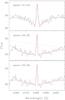 |
Fig. 3 Comparison between the simultaneous fit to the absorption and emission components of the Hγ line for two spaxels in Tololo 1937-423. Upper panel: spectrum of spaxel (21, 22) around Hγ, together with the best fit (red solid line; the dashed green line represents the fitted continuum). Here the unconstrained fit provides a good match to the line profile. Central panel: unconstrained fit to spaxel (22, 18), which clearly fails to fit the continuum and overestimates the absorption component. Bottom panel: constrained fit, which is more physically sound, while yielding a slightly higher χ2 value. |
The continuum (typically 30–50 Å on both sides) was fitted by a straight line. Lines in a doublet were fit by imposing that they have the same redshift, width, and a fixed flux ratio equal to 3 for [N ii] and [O iii].
Criteria such as flux, error on flux, velocity, and width were used to do a first, automatic assessment of whether to accept or reject a fit. For instance, lines much narrower or much wider than the instrumental width were flagged as rejected, as were lines with an error on the flux more than about 20% of the flux (the exact limits depend on the specific line and on the overall quality of the spectrum). Such criteria were complemented by a visual inspection of all fits, which led to overriding, in a few cases, the decision by automated criteria (either accept a fit flagged as rejected, or vice-versa). For instance, sometimes the program fit large noise spikes for very faint or even completely absent emission lines; in other cases, a particularly noisy continuum or bad pixels decreased the computed S/N below the acceptance threshold, while the actual fit was clearly good enough. For those galaxies where no absorption component was fit, the measured intensities of the Balmer lines are, strictly speaking, lower limits to the actual values.
2.5. Creating the 2D maps
The emission-line fit procedure gives, for each line and for each line parameter (for instance flux), a table with the fiber ID, the measured value and the acceptance/rejection flag. This table was then used to produce a 2D map, by using an IRAF script that takes advantage of the fact that the combined VIMOS data are arranged in a regular 44 × 44 matrix.
Line ratios maps for lines falling in the wavelength range of either grism, were simply derived by dividing the corresponding flux maps. The Hα/Hβ line ratio was computed after registering and shifting the Hα map to spatially match the Hβ map.
Continuum maps were obtained by summing the flux within specific wavelength intervals, which were selected so as to avoid strong emission lines or residuals from the sky spectrum subtraction. Since a polynomial fit with a sigma-clipping algorithm was carried out to compute the continuum intensity, the results are unaffected by faint emission lines, skyline residuals, or cosmic ray hits.
3. Results
3.1. Morphology of the ionized gas and of the stellar component
We produced continuum-subtracted intensity maps of the brighter emission lines, which for most of the galaxies include Hγ, Hβ, [O iii] λ5007, He iλ5876, Hα, [N ii] λ6584, [S ii] λ6717, 6731, and [Ar iii] λ7136. The emission-line maps trace the ionized phase of the interstellar gas. This comprises gas photoionized by ultraviolet photons from hot stars and collisionally ionized gas, i.e., regions that have been shock-heated to temperatures T> 106 K by blastwaves from supernova explosions. These maps therefore provide information about the location and size of the individual H ii regions, and allow curvilinear structures to be identified, such as bubbles, shells, or filaments, which are typical footprints of supernova-driven winds.
“Pure” continuum maps, i.e., continuum maps free of emission lines, were also built in different spectral zones. The continuum maps trace the stellar component of the galaxies; the comparison of the ionized gas distribution and the continuum maps provides insight into the spatial distribution of the different stellar populations. Continuum-subtracted emission-line maps and continuum maps of the galaxies are displayed in Figs. 6 to 13.
Seven out of the eight observed galaxies exhibit an irregular morphology in emission lines, with the starburst activity spread over several clumps. After applying the BCGs classification proposed in Cairós et al. (2001a), which is based on the position and morphology of the SF regions, these seven objects fit in the category of “Extended” starburst. Only the galaxy Tololo 0127-397 with a single, central H ii region corresponds to the “Nucleated” starburst class (see Table 1). Filaments and curvilinear structures of ionized gas are frequent, in particular at low surface brightness levels. Such structures, commonly referred to as “bubbles”, “super-bubbles”, “holes”, or “shells”, are common among SF dwarf galaxies (Martin 1997).
In the continuum, the galaxies also display a wide range of patterns. Five of the objects, Haro 11, Haro 15, Tololo 1924-416, Tololo 1937-423 and Mrk 900 exhibit an irregular morphology at all surface brightness levels; the distorted isophotes at low surface brightness levels, the presence of faint tails, and the multiple nuclei (in Haro 11 and Haro 15) are in good agreement with the hypothesis of their being interacting galaxies. Haro 14, Tololo 0127-397, and Mrk 1131 each display a single nucleus and elliptical, regular isophotes.
In seven out of the eight mapped objects (all but Tololo 0127-397), the distribution of the gaseous emission strongly differs from that of the stellar component. This probably indicates of the presence of different stellar populations or of an inhomogeneous dust distribution (or, possibly, both).
3.2. Ionization: mechanism and structure
Three main different mechanisms can be responsible for the ionization of emitting-line galaxy regions: photoionization due to ultraviolet (UV) photons from hot stars, photoionization by a power-law continuum source from AGN, and shock-ionization, which is the collisional ionization that takes place in shocks caused by stellar winds and supernovae. To probe the dominant ionization mechanism in galaxies, diagnostic diagrams involving excitation-dependent, extinction-independent line ratios have been commonly used (Baldwin et al. 1981; Veilleux & Osterbrock 1987). The most common diagnostic plots are [O iii] λ5007/Hβ versus either [N ii] λ6584/Hα, or [S ii] λλ6717, 6731/Hα, or [O i] λ6300/Hα.
The [O iii] λ5007/Hβ emission-line ratio is primarily an excitation parameter indicator, and it provides information about the available fraction of hard ionizing photons of the ionizing star cluster embedded in the nebula; thus, a large [O iii] λ5007/Hβ ratio indicates a highly ionized region.
[N ii] λ6584 and [S ii] λλ6717, 6731 are low ionization lines, which arise in a zone of partially ionized hydrogen. This low-ionization zone is quite extended in objects that are photoionized by a spectrum containing a large fraction of high-energy photons, but is nearly absent in galaxies photoionized by OB stars. Accordingly, high [N ii] λ6584/Hα, or [S ii] λλ6717, 6731/Hα ratios usually indicate the presence of ionizing mechanisms other than photoionization from hot stars, e.g. shock waves and/or AGN.
The [O iii] λ5007/Hβ, [N ii] λ6584/Hα, [S ii] λλ6717, 6731/Hα, and [O i] λ6300/Hα maps were built as the first step toward a better understanding of the ionization mechanism acting in the observed galaxies. Results are displayed in Figs. 6 to 13. As expected, the ionization is produced predominantly by UV photons from hot stars. Higher values of [O i] λ6300/Hα and/or [S ii] λλ6717, 6731/Hα in the outer galaxy regions also suggest a contribution by shocks in six out of the eight sample galaxies, Haro 11, Haro 14, Tololo 0127-397, Tololo 1924-416, Tololo 1937-423 and Mrk 900.
3.3. Interstellar extinction
Interstellar extinction can be probed by comparing the observed ratios of hydrogen recombination lines with their theoretical values (Osterbrock & Ferland 2006). In the optical domain, the extinction is derived from the ratio of the different H i Balmer line series to Hβ. We computed AV from the Hα/Hβ ratio, except for Haro 15, where it was derived from Hβ/Hγ and Mrk 1131, for which we only have the orange spectrum. We adopted the Case B, low-density limit, T = 10 000 K approximation (Osterbrock & Ferland 2006), and used the Cardelli et al. (1989) extinction law. Results are displayed in Figs. 6 to 13.
All the sample objects display a significant amount of dust and complex extinction patterns; the nonuniform dust distribution emphasizes the importance of performing a bidimensional study of the interstellar extinction: just assuming a single, spatially constant value for the extinction, as is usually done, can lead to large errors in deriving the photometric parameters of the galaxies.
3.4. Electron density distribution
The electron density, Ne, in an H ii region can be derived by observing the effects of collisional deexcitation. The most often used line ratio is [S ii] λ6717/[S ii] λ6731, a sensitive diagnostic for the electron density range 100 to 10 000 cm-3. Maps of the [S ii] λ6717/[S ii] λ6731 for the galaxy sample are displayed in Figs. 6 to 13. The values of the density are below the low-density limit for all the objects except Tololo 0127-397.
3.5. Ionized gas kinematics
The kinematics of the ionized gas were obtained by fitting a single Gaussian to the Hα emission line, except for Haro 15, for which the [O iii] λ5007 was fit. No attempts were made to decompose the line profile into multiple components, even when it shows significant deviations from a Gaussian. (A more detailed analysis of the kinematics of our objects will be presented in a forthcoming paper.)
Velocity dispersions were obtained from the measured line widths by subtracting the instrumental width in quadrature. The uncertainty on the latter is about 2 km s-1 FWHM (Sect. 2.3), so close to the uncertainty on the measured width in the brightest spaxels, which means that the derived uncertainty on the computed velocity dispersion, σ, is about 10–15 km s-1 for low values of σ, and decreases as σ increases.
3.6. Integrated spectroscopy
For each galaxy, we extracted a one-dimensional spectrum of the main SF regions. For Tololo 0127-397, Tololo 1937-423, and Mrk 1131, we produced just one spectrum integrated over the main, central SF region. In Mrk 900 we obtained a spectrum by integrating over the three brightest knots, a, b, and c; in Haro 14 we produced a summed spectrum for each of the two brightest knots, e and b; in Haro 15, we produced two integrated spectra, one for knot b and one for knots a1 through a4, and two spectra for Tololo 1924-416, for knots b and a. In Haro 11 we extracted three spectra, one for each of the three SF regions.
Because of the heterogeneity of the sample in terms of apparent luminosity, distance, morphology, brightness of the SF regions, and S/N of the observed spectra, there is no unique, clear-cut criterion for defining the limits of the SF regions. Thus we followed a pragmatic approach based on the specific morphology of the SF knots: we integrated the flux within an area whose boundary follows the shape of the SF knot with a minimum area of ~15 square arcsec (that is, with an equivalent radius larger than the seeing FHWM). The integration areas are shown in the [N ii] maps in Figs. 6 to 13 (except for Haro 15, where they are shown in the Hβ map). We also produced an integrated spectrum for the whole galaxy by summing over all spaxels with measurable Hα and Hβ emission (only Hβ for Haro 15 and only Hα for Mrk 1131).
3.7. Check on flux calibration
In order to check the accuracy of the flux calibration of our spectra, we compared the observed ratios of the emission line fluxes over the Hβ flux with literature data. For Haro 11, we compared with the results published in James et al. (2013) and in Guseva et al. (2012). For the former we extracted an integrated spectrum within the same area as used by James et al. (2013) for their integrated spectrum data shown in their Table 3. Also, we obtained the integrated spectrum for knot b by computing the combined flux ratios from the values for the C1 and C2 components listed in their Table A2. As for Guseva et al. (2012), we extracted two integrated spectra within a 3 × 3 spaxel region centered on knots b and c, which corresponds roughly to the integration area used in their spectra, and compared the observed flux ratios with those listed in their Table 2. (Since we are comparing flux ratios and not absolute fluxes, small differences in the integration area or its exact position will only produce second-order effects.)
Flux ratios for Haro 14 were obtained by integrating over all spaxels with detected Hα and Hβ emission, and compared with those published by Moustakas & Kennicutt (2006), after removing their correction for galactic extinction. Flux ratios for Tololo 1924-416 were measured on a spectrum obtained by integrating over a 3 × 3 spaxel region centered on the continuum peak (Guseva et al. 2012 refer to “the brightest part of ESO 338-IG 004”) and compared with those published in Table 1 of Guseva et al. (2012).
The results are shown in Fig. 4. The data from James et al. (2013) are in strong disagreement with both our data and those published by Guseva et al. (2012) for the same object, which can hardly be attributed to calibration, to line measurement uncertainties, or to the different apertures used to obtain the line fluxes; it suggests instead some sort of systematic error in their flux calibration. Aside from James et al. (2013) data, there is a broad, fair agreement between the literature data and ours, with no evident systematic effects. The scatter of the datapoints (excluding Hβ and James et al. (2013) datapoints) is 0.12.
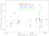 |
Fig. 4 Ratio between the flux measured on our spectra with those published in the literature (all fluxes normalized to that of Hβ), plotted against the lines’ restframe wavelength. M&K2006: Moustakas & Kennicutt (2006); G2012: Guseva et al. (2012); J2013: James et al. (2013). The vertical dashed lines mark the location of the Hβ and Hα emission lines. |
Reddening-corrected line-intensity ratios.
3.8. Line flux measurement and extinction coefficient
Fluxes of the most important emission lines were measured using the splot task in IRAF. We usually fitted a Gaussian to the line profile, except for Haro 11, whose emission lines have clearly non-Gaussian profiles: their fluxes were obtained by integrating the line profile (key “e” in splot). Statistical errors on the line fluxes measurements were computed using the expression provided in Pérez-Montero et al. (2009). In those cases in which absorption wings around the Balmer lines are present, we simultaneously fit an absorption and an emission component.
As for calibration uncertainties, lacking any estimate of the flux calibration uncertainty as a function of wavelength, we followed a practical approach based on the flux calibration check described above. We expect flux ratios of nearby lines, such as the [O iii] doublet over Hβ, to be relatively insensitive to flux calibration errors; on the contrary, flux ratios of far apart lines, such as Hδ/Hβ or Hα/Hβ, will carry much larger uncertainties. We thus made the simple assumption that the uncertainties on the emission line fluxes, normalized to Hβ, scale linearly with the difference in wavelength between the line and Hβ, assigning a 8% error to Hα/Hβ and a 6% error to Hβ/Hδ (with a minimum of 1% on the ratios of nearby lines).
When the absorption wings around the Balmer lines are not visible, we assumed that the equivalent width in absorption is the same for all the lines. We first adopted an initial estimate for the absorption equivalent width, EWabs, corrected the measured fluxes, and computed the extinction coefficient C(Hβ) through a least-square fit to the Balmer emission-line decrement. We then varied the value of EWabs, until we found the one that provides the best match (e.g., the minimum scatter in the fit) between the corrected and the theoretical line ratios.
In general, the extinction-corrected Balmer line ratios are within a few percentage points of their theoretical value, with this small discrepancy probably explained away by the uncertainties on the flux calibration in our data and by departures of the actual dust distribution from a simple background screen geometry. The exception is Haro 11, where extinction-corrected and theoretical Balmer line ratios are off by as much as 10%. Such a large variance is likely due to the line emission in this galaxy being the superposition of distinct kinematical components, with also different chemical compositions, and to the presence of a stellar component with a P Cyg profile in the Hα line (Guseva et al. 2012; James et al. 2013).
Extinction-corrected line fluxes (normalized to Hβ = 100), the extinction coefficient C(Hβ), the Hβ extinction-corrected flux, and the equivalent widths of the absorption components in the Balmer line (in those case where they could be fit), are listed in Table 3 for all galaxies except Mrk 1131. For the latter, which lacks the blue grism spectra, we list the observed emission line fluxes, as well as the log (N+/ H+) and log (S+/ H+) ratios and the electron density Ne, in Table 5.
3.9. Physical parameters, diagnostic-line ratios, and chemical abundances
Temperature and metal abundances were derived using the relevant formula in Izotov et al. (2006b). Since our spectra miss the [O ii] λ3727 doublet, we could not derive the oxygen abundance. Electron densities were computed from the [S ii] λ6717 /λ6731 line ratio using the task temdem in the IRAF nebular package. Table 4 lists the most important line ratios for diagnostic, the electron temperature, and the electron density, as well as the derived ionic abundances for O2 +, N+, and S+.
To explore the ionization mechanism acting in the galaxies, we plotted the emission-line ratios for the integrated spectra, as well as for the spectra of the brighter SF knots, in the diagnostic diagrams [O iii] λ5007/Hβ versus [N ii] λ6584/Hα, [S ii] λλ6717, 6731/Hα, and [O i] λ6300/Hα (see Fig. 5). The empirical boundaries between the different zones (from Veilleux & Osterbrock 1987) and the theoretical boundaries proposed by Kewley et al. (2001) are also shown in the plot. In the three diagrams, all the galaxies (and the selected SF regions) fall within the regions occupied by H ii regions.
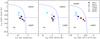 |
Fig. 5 Optical emission-line diagnostic diagrams, separating Seyfert galaxies and LINERS from HII line objects. Integrated spectra are represented by filled symbols. Solid lines are the empirical borders from Veilleux & Osterbrock (1987), while dotted lines are the theoretical borders from Kewley et al. (2001). |
Physical conditions and ionic abundances.
Line fluxes for Mrk 1131.
4. Comments on individual objects
4.1. Haro 11 (=ESO 350-IG038)
Haro 11 is a luminous BCG which has been widely studied over a wide frequency range from X-rays to radio (see Cormier et al. 2012 and references therein). Optical spectroscopy and surface brightness photometry in the optical and near-infrared (NIR) was published by Bergvall & Östlin (2002). Haro 11 exhibits an intricate morphology with three main SF knots, which contain numerous super star clusters with ages between 1 and 40 Myr (Adamo et al. 2010). Fabry-Perot observations show that the galaxy presents a complex velocity field, which together with the distorted morphology, has been interpreted in terms of a merger event (Östlin et al. 1999, 2001). An IR luminosity of 1.9 × 10¹¹L⊙ classifies Haro 11 as a luminous IR galaxy (LIRGs; Engelbracht et al. 2005). It is also a Lyα and Lyman-continuum emitter (Hayes et al. 2007), which has been regarded as a Lyman break analog – the very rare population of local galaxies that strongly resemble the properties of the high-z LBGs (Grimes et al. 2007; Overzier et al. 2008). FUV FUSE observations are presented in Bergvall et al. (2006) and Grimes et al. (2009).
Abundances have recently been measured using VLT/X-shooter observations (Guseva et al. 2012). The values found for the two major H ii regions, 12 + log (O / H) = 8.33 ± 0.01 and 12 + log (O / H) = 8.10 ± 0.04 are considerably higher than the value of 12 + log (O / H) = 7.9 reported in Bergvall & Östlin (2002), and they shift the metallicity value from ≈1/6 to 1/3 Z⊙. Dynamical and chemical results based on spatially resolved VLT/FLAMES spectroscopy have been recently published by James et al. (2013).
Two-dimensional maps of Haro 11 are shown in Fig. 6. At the Haro 11 distance, the fiber diameter provides a spatial sampling of 273 pc. The emission-line maps reveal an irregular central region, consisting of three major SF knots roughly arranged in an “L-shaped” structure. These knots (labeled a, b, and c in the continuum map in Fig. 6 following Kunth et al. 2003) are surrounded by a nearly circular extended halo. All the emission-line maps display the same pattern, but in the [O i] λ6300 map, a small curvilinear feature extending eastward from knot c becomes visible (see also the [O i] λ6300/Hα ratio map), though it is not evident in the other maps. Several ionized filaments to the south are conspicuous in the more extended maps (marked by arrows in the Hβ map). Knots a and b are depicted well in the auroral line [O iii] λ4363; in both knots, we also detected the high-ionization He iiλ4686 Å line, which is characteristic of Wolf-Rayet (WR) galaxies (Conti 1991). The spaxels in which He iiλ4686 Å is visible are marked in the [O iii] λ5007 map.
The stellar morphology comes close to that of the ionized gas; however, in the continuum maps, the light distribution peaks on knot c, the faintest knot in line emission, while knot b, the brighter line emitter, is weak in the continuum. This points to a different stellar content between the major knots.
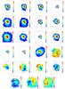 |
Fig. 6 Emission-line fluxes, continuum, line ratios, and ionized gas kinematics maps for Haro 11. Knots are labeled in the continuum map following Kunth et al. (2003). Spaxels where the WR bump has been detected are outlined in the [O iii] λ5007 map. Continuum contours are overlaid on the Hα map; [O iii] λ5007 contours are overlaid on the [O iii] λ5007/Hβ map (in both maps contours are spaced 0.4 dex apart).The regions inside which spaxels were summed to obtain the integrated spectrum of the SF knots are outlined in the [N ii] λ6584 map. The arrows show the location of the filaments mentioned in the text (Sect. 4.1). The angular scale is 407 pc arcsec-1. North is up, east to the left. Axis units are arcseconds. Flux units are 10-18 erg s-1 cm-2 (per 0.67 × 0.67 arcsec2 spaxel). Velocity units are km s-1. |
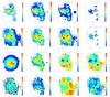 |
Fig. 7 Haro 14. The angular scale is 63 pc arcsec-1. Knots are labeled on the Hβ flux map. The solid white line in the Hβ map traces the curvilinear structure described in Sect. 4.2. |
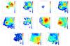 |
Fig. 8 Haro 15. This galaxy was only observed with the blue grism. Continuum contours are overplotted on the Hγ map. The integration areas for the summed spectra of the SF knots are outlined in the Hβ map. The solid curved lines in the [O iii] map trace the curvilinear features mentioned in Sect. 4.3. The angular scale is 416 pc arcsec-1. |
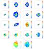 |
Fig. 9 Tololo 0127-397. The angular scale is 346 pc arcsec-1. The curved white solid lines in the Hα map show the filaments described in Sect. 4.4. |
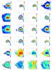 |
Fig. 10 Tololo 1924-416. The angular scale is 206 pc arcsec-1. The curved white solid lines in the Hα map traces the tails stretching out from the center, as described in Sect. 4.5. |
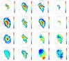 |
Fig. 11 Tololo 1937-423. The angular scale is 199 pc arcsec-1. The curves solid lines in the [S ii] map traces the curvilinear features described in Sect. 4.6. |
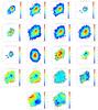 |
Fig. 12 Mrk 900. The angular scale is 92 pc arcsec-1. |
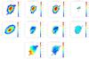 |
Fig. 13 Mrk 1131. This galaxy was observed only with the orange grism. The angular scale is 156 pc arcsec-1. |
The ionization maps display an intricate pattern. In the western galaxy regions, the [O iii] λ5007/Hβ ratio displays high values with several local maxima. The position of two of these local peaks coincides with the position of knots a and b, the bigger line emitters. In the other line-ratio maps, knots a and b are minima, as expected in regions photoionized by OB stars; the values of the line ratios in this galaxy region are consistent with photoionization by hot stars (Veilleux & Osterbrock 1987). The eastern galaxy area shows a strong gradient in [O iii] λ5007/Hβ, with values decreasing from south to north. The ratios of [O i] λ6300, [N ii] λ6584, and [S ii] λλ6717, 6731 with Hα show a strong gradient in a southwest-northeast direction, reaching a maximum on the northeast edge. The high values of [O i] λ6300/Hα (log [ O i ] λ6300 / Hα ≥ −1) and [S ii] λλ6717, 6731/Hα (log [ S ii ] λλ6717, 6731 / Hα ≥ −0.4) in that regions indicate that an additional ionization mechanism (most probably shocks) is acting there.
The extinction also displays a patchy pattern; local peaks in the interstellar extinction with values of AV about 2 are reached close to the SF knots b and c. An extinction patch or lane located between the SF knots has been observed in several BCGs (e.g., García-Lorenzo et al. 2008; Vanzi et al. 2008; Cairós et al. 2009b) and could be related to the sweeping out of the ISM by stellar winds and SNs.
The distribution of the electron density, Ne, is also irregular. The lowest values of the [S ii] λ6717 /λ6731 ratio (the highest values of the electron density) are reached in the central galaxy regions on knot b and southeast of it, and the line ratio increases slightly outwards, except in the northeast, where there is also a region with lower values of the [S ii] λ6717 /λ6731 ratio. Taken at face value, the values of the electron density are below the low density limit (Ne ≈ 100 cm-3) in the whole covered area.
We should note that the [S ii] λ6731 falls on a telluric absorption feature, so its measured flux is somewhat smaller than the actual value. However, at a first-order approximation, this effect is spatially independent, so the patterns seen in the [S ii] λ6717 /λ6731 and the [S ii]/Hα maps are real.
The galaxy displays quite an irregular velocity field with an amplitude of about 200 km s-1. The minimum value (V ≃ 6060 km s-1) is reached on the eastern edge, while the maximum in radial velocity is located about 2 arcsec northwest of knot b. The velocity dispersion map shows several local minima with σ ≃ 60 km s-1 and values varying up to about 130 km s-1 with the maximum located southeast of the central line-emitting region.
Line profiles show significant deviations from a single Gaussian, which was already pointed out by Östlin et al. (1999). The velocities measured in a 3 × 3 spaxel box (2″ × 2″) centered on knots a, b, and c (6253, 6175, and 6143 km s-1, respectively) agree closely with the observed velocities published by Sandberg et al. (2013), after allowing for an offset of about 25 km s-1 (which can be readily explained if no heliocentric velocity correction was applied to their data).
We produced the integrated spectrum of the galaxy, as well as the integrated spectra of the three major SF regions a, b, and c. The representative spectrum shown in Fig. 2 displays a typical high ionization H ii spectrum, with strong Balmer recombination lines and very prominent collisional-excited [O iii] lines atop a blue continuum. Extinction-corrected line fluxes and equivalent widths, and the derived line ratios, physical parameters, and abundances of the brighter emission lines are shown in Tables 3 and 4, respectively.
The high values of the equivalent widths of the recombination lines in knots a and b (e.g., W(Hα) ≥ 600), and the detection of the high-ionization He iiλ4686 Å line, are in good agreement with the young ages reported for these knots in Adamo et al. (2010). Emission-line ratios for the galaxy and for the three knots are plotted on the diagnostic-diagram in Fig. 5. The galaxy and the knots fall within the regions occupied by H ii regions.
4.2. Haro 14 (=NGC 0244)
Haro 14 is a relatively metal-rich (Z = Z⊙/ 3; Hunter & Hoffman 1999) dwarf galaxy included in the Vorontsov-Velyaminov (1977) atlas of interacting systems. Surface photometry in the optical (Marlowe et al. 1997; Doublier et al. 1999; Gil de Paz et al. 2003; Gil de Paz & Madore 2005; Hunter & Elmegreen 2006) and in the NIR (Doublier et al. 2001; Noeske et al. 2003) has shown that this system is made of a central starburst and an extended almost circular, older stellar component.
Maps of emission-line fluxes, line ratios, and kinematics are shown in Fig. 7. The spatial sampling is 42 pc per spaxel. Haro 14 displays a rather intriguing morphological pattern. In the emission-line maps several SF knots (labeled as a, b, c, d in Hβ in Fig. 7) are visible, arranged in a “bar-like” structure along the north-south direction. A bubble-like curvilinear feature (labeled as e and traced by a solid curved line) departs from the central “bar-like” formation and extends about  (735 pc) eastwards; although its morphology is suggestive of a supergiant shell, no kinematical evidence of superwinds were found in the Fabry-Perot images analyzed in Marlowe et al. (1997). A small ionized gas condensation is also apparent in the west. All the emission-line maps display a similar pattern.
In the continuum map, Haro 14 displays a largely different morphology with a central complex of knots, encircled by a very regular, almost circular envelope. This central region is off-center with respect to the outermost isophotes of the galaxy, and the position of the continuum peak does not coincide with the position of any of the SF knots detected in the emission-line maps, but is located about 2″ (about 125 pc) south of knot c (the emission peak in the emission-line frames). These maps indicate the presence of at least two different stellar populations: a recent episode of star formation, and an underlying, more evolved stellar component.
Diagnostic emission-line maps, are displayed in Fig. 7 (line three). The fit of the line [O i] λ6300 is affected by residuals of the [O i] λ6300 skyline subtraction, so maps of the [O i] λ6300/Hα line ratio could not be produced. In the three diagnostic emission-line maps, the SF knots appear to be delineated very well, and the peaks in [O iii] λ5007/Hα roughly coincide with the minima in [N ii] λ6584/Hα and [S ii] λλ6717, 6731/Hα, as expected in regions photoionized by stars. The values of the diagnostic-line ratios are also consistent with ionization from OB stars, but in the [S ii] λλ6717, 6731/Hα map in the southern outskirts of the galaxy: here high values ([S ii] λλ6717, 6731/Hα≥−0.3) indicate that another ionization mechanism (most probably shocks) is playing an important role there.
The electron density distribution is nearly constant, with values close to the low density limit in the whole area. There are maxima of the density (minima in the maps) at the SF knots position. The dust distribution is inhomogeneous, and the interstellar extinction peaks in the southeastern galaxy regions with values of AV up to about 2. The galaxy displays an irregular velocity field with low amplitude (less than 60 km s-1). The velocity dispersion map shows a wavy pattern with values ranging from about 5 to 40 km s-1.
We produced both the integrated spectrum of the galaxy and the spectra of the two major SF regions b and e. The spectrum of the galaxy displayed in Fig. 2 is nearly flat, which is typical of high-ionization H ii regions. Absorption wings underneath the Balmer emission lines are clearly visible on Hγ and Hβ. Extinction-corrected line fluxes and equivalent widths, along with the derived line ratios, physical parameters, and abundances of the brighter emission lines, are shown in Tables 3 and 4, respectively.
In the diagnostic-diagram (Fig. 5), the line ratios for the galaxy and the SF knots fall within the area occupied by H ii regions. The extinction that we derived for the integrated spectrum, E(B − V) = 0.24, is slightly below the mean extinction provided in Hunter & Hoffman (1999), E(B − V) = 0.35.
4.3. Haro 15 (=Mrk 960)
Haro 15 belongs to the catalog of galaxies with multiple nuclei published by Mazzarella & Boroson (1993). It appears classified as “strongly interacting separated galaxies, or a single highly perturbed system which may be an advanced merger”: two separated nuclei are clearly distinguished in the center of a more regular envelope (Mazzarella et al. 1991). Optical broad- and narrow-band surface photometry is presented in Cairós et al. (2001a,b). In-depth spectroscopy studies have been published in the series of papers by Kong (2004), Shi et al. (2005, and references therein), and López-Sánchez & Esteban (2010, and references therein). Shi et al. (2005) derived an overall average oxygen abundance 12 + log (O / H) = 8.33. Analyses focused on the kinematics and the physical properties of Haro 15 have been recently published by Firpo et al. (2011) and Hägele et al. (2012), respectively. Haro 15 appears listed as a WR galaxy in (Schaerer et al. 1999), because of the detection of the He iiλ4686 emission line by Kovo & Contini (1999).
We collected data for Haro 15 only with the blue-grism. Maps of emission-line fluxes, emission-line ratios, and ionized gas kinematics are shown in Fig. 8. The spatial sampling is about 279 pc per spaxel.
The VIMOS FOV encompasses a large fraction of the central starburst, which includes the two major emitters (labeled as a and b in Fig. 8 following Cairós et al. 2001a; knot a has been resolved into smaller SF entities in the emission-line maps). All emission-line maps, except [O iii] λ4363, display the same morphology: the northwestern region (a) is resolved in an ensemble of SF regions, forming a ring-like pattern, which seems to connect with the big line emitter b, at the southwest. The [O iii] λ4363 auroral emission line is detected only in knot b, in which the WR bump has also been identified (see the [O iii] map in Fig. 8). The presence of high-excitation lines in knot b is consistent with the higher values we find for Hβ, as well as with the blue color (U − B = −0.73) reported in Cairós et al. (2001a). Curvilinear structures resembling bubbles extend to the north and to the southwest (marked in the Hβ map).
The continuum map shows a different pattern: the peak of emission is located on knot a, which appears as a single emitter, surrounded by notably boxy isophotes; the dust in the central regions is evident. The morphology in emission-line and continuum can again be either the result of an age difference or an effect of a highly inhomogeneous dust distribution, most probably a combination of both factors.
In the [O iii] λ5007/Hβ line-ratio knot a is very well delineated. The high values of the excitation (log [O iii] λ5007/Hβ≥ 1) are in good agreement with the detection of high ionization lines (WR features and [O iii] λ4363) in this knot. The ratio values in the mapped FOV are consistent with ionization by hot stars. The extinction shows an inhomogeneous pattern, with the higher values of the extinction located between the SF knots.
The gas velocity map shows an overall rotation, roughly around an axis oriented northwest-southeast, though with clearly distorted isovelocity contours. The maximum amplitude is about 160 km s-1. The velocity dispersion map is irregular, with a local minimum coinciding with the brightest knot and values ranging from about 25 to 70 km s-1.
We produced the integrated galaxy spectrum, and the integrated spectra of the two major SF regions a and b. The galaxy spectrum displayed in Fig. 2 shows a continuum rising blueward, indicating the presence of OB stars. Marked absorption wings are detected around Hδ, Hγ, and Hβ. Extinction-corrected line fluxes and equivalent widths, and the derived line ratios, physical parameters and abundances of the brighter emission lines are shown in Tables 3 and 4, respectively.
There is a significant difference between the ionization parameter and abundances found in knots a and b. The two nuclei and the difference in their abundances, the boxyness of the isophotes, the presence of dust in the central regions, and the distorted velocity field, all support the hypothesis of a merger for this galaxy (López-Sánchez & Esteban 2009).
4.4. Tololo 0127-397
Tololo 0127-397 is a compact object, with regular, elliptical isophotes and a single centered burst. Optical surface brightness photometry is presented in Cairós et al. (2001b,a). In Schaerer et al. (1999) it is cited as a possible WR galaxy. Maps of emission-line fluxes, line ratios, and ionized gas velocity and velocity dispersion are shown in Fig. 9. At the Tololo 0127-397 distance, the fiber size provides a spatial sampling of 232 pc.
The emission-line maps display a unique, very compact, almost circular central SF region; however, the emission is irregular at lower surface brightness levels, and filaments extending northward and eastward are very visible (depicted in the Hα map). All emission lines display the same pattern. The presence of the broad-band He iiλ4686 line, a signature of WR stars, is confirmed: the position of the spaxels with a clear detection is marked in the [O iii] map (Fig. 9).
The continuum exhibits a similar morphology, but the stellar distribution presents a regular, elliptical low-surface brightness envelope. The continuum intensity peak, which spatially coincides with the peak in emission lines, is located in the center of the outer elliptical isophotes.
All the four ionization maps show the same structure and trace the central starburst, as expected for regions ionized by hot stars. The high values of the [S ii] λλ6717, 6731/Hα line-ratio in the outer galaxy regions (log [S ii] λλ6717, 6731/Hα≥ −0.4) suggest that another mechanism, most probably shocks, could play a significant role there.
The extinction map is irregular, with relatively high values (AV up to 1.5) in the eastern galaxy regions. The density distribution is roughly constant over the whole mapped area. The values of the [S ii] λλ6717, 6731 are about 1.2 in the central regions, and they decrease slightly outward, where they reach the value of the low-density limit.
Tololo 0127-397’s kinematics display an overall rotation about an axis oriented northeast-southwest, with an amplitude of about 60–70 km s-1; however, some waviness is clearly visible in the velocity map. The velocity dispersion is lowest in the inner region with σ ≃ 40 km s-1 and increases to about 60–70 km s-1 in the outer regions.
The heliocentric velocity we derived (cz ≃ 5215 km s-1) differs significantly from the value published in NED, which is based on a single datapoint: the measurement by Terlevich et al. (1991), which lists this object as having redshift z = 0.016 (their Table 2). Our value is in good agreement with the one (z = 0.01735) published by Bordalo & Telles (2011).
Figure 2 shows a flat spectrum, with prominent emission-lines, characteristic of a high-ionization H ii region. The diagnostic line ratios fall within the area occupied by H ii regions in the diagnostic-diagram (Fig. 5).
4.5. Tololo 1924-416 (=ESO 338-IG004)
Tololo 1924-416 is a well known luminous BCG, which was first studied in detail in Bergvall (1985) and Iye et al. (1987). The optical emission is dominated by a central starburst region, which has been resolved into compact star clusters in HST images (Meurer et al. 1995; Östlin et al. 1998). Optical and NIR images (Doublier et al. 1999; Bergvall & Östlin 2002; Gil de Paz et al. 2003; Gil de Paz & Madore 2005) have shown that the SF regions are placed atop a very elongated and much redder elliptical host. The dynamics of the ionized gas was studied in Östlin et al. (1999, 2001), where the complex velocity field was interpreted in terms of a merger; further evidences for the merger hypothesis were raised from the study of the galaxy stellar dynamics by means of observations of the Ca ii-triplet in the NIR (Cumming et al. 2008). The Lyα morphology of the galaxy has been discussed in Hayes et al. (2005) and Östlin et al. (2009). The oxygen abundance based on recent VLT/X-shooter observations, 12 + log (O / H) = 7.89 ± 0.01 (Guseva et al. 2012) is slightly lower than the previous findings, which are in the range 7.92–8.08 (Masegosa et al. 1994; Bergvall 1985; Bergvall & Östlin 2002). It appears classified as a WR galaxy in Schaerer et al. (1999). This galaxy has a companion at a projected distance of 70 kpc to the south-west (Östlin et al. 2001).
Maps of emission-line fluxes, emission-line ratios and kinematics are shown in Fig. 10. The spatial sampling is about 138 pc per spaxel. Tololo 1924-416 presents the same morphology in all the mapped emission lines. The SF activity takes place in the central galaxy regions, where two major H ii regions – labeled a and b in Fig. 10 – are aligned with the galaxy major axis (east-west). A tail stretches out from the center eastward, roughly aligned with the central blobs, while another extends out toward the northwest (as indicated in the Hα map). The WR signature is identified across the central starburst and the position of the spaxels with clear WR detection is marked in Fig. 10.
A unique central knot is distinguished in the continuum map, located approximately between the two major knots detected in the emission-line frames. The difference between the stellar and ionized gas morphology probably reflects the existence of two stellar populations.
The central starburst region displays the same pattern in the three derived emission-line ratio maps. The SF knots are well delineated, and [O iii] λ5007/Hβ peaks where [N ii] λ6584/Hα and [S ii] λλ6717, 6731/Hα have a minimum, as expected in regions ionized by hot stars. The values of the lines ratio are consistent with photoionization by hot stars, except in the eastern and southern galaxy outskirts, where the higher values of [S ii] λλ6717, 6731/Hα suggest the presence of shocks.
The galaxy displays an inhomogeneous extinction pattern, with the extinction values increasing outward. The extinction peaks (AV ≈ 2) are located on a dust lane that extends north to south, east of knot a. The electron density distribution is inhomogeneous as well, because the [S ii] line ratio has values close to one in the center (in the SF regions) and increases outward (meaning that the electron density decreases).
The galaxy exhibits an irregular velocity field, very unlike the line-intensity maps, with a minimum cz ≃ 2810 km s-1 east of the big Hα region, and a number of local maxima with velocity cz ≃ 2870 km s-1 on the west side of the galaxy. The velocity dispersion field is highly irregular, too, with features that apparently have little or no relation to those in the velocity field. The lowest σ, 20 km s-1, is achieved in the western edge of the map, colocated spatially with the small enhancement in Hα flux. In general, there seems to be an anticorrelation between line-emission flux and velocity dispersion. There also are several local maxima, away from the peaks in line emission, where σ reaches about 65 km s-1. The radial velocity measured in a 3 × 3 spaxel box (2″ × 2″) centered on the emission peak, 2851 km s-1, agrees well with the value published by Sandberg et al. (2013).
We generated the integrated spectrum of the galaxy and the integrated spectrum of the two major SF regions a and b. As seen in Fig. 2, Tololo 1924-416 has a very flat spectrum with prominent recombination lines and [O iii] lines, which are characteristic of a high-ionization H ii region. Extinction-corrected line fluxes and equivalent widths, as well as the derived line ratios, physical parameters, and abundances of the brighter emission lines are shown in Tables 3 and 4, respectively. H ii-like ionization is the dominant mechanism in the galaxy (see Fig. 5). There is no significant difference between the ionization parameter and abundances that we find for knots a and b.
4.6. Tololo 1937-423
Tololo 1937-423 is an intriguing object that has not been studied much so far. It is made up of a very irregular starburst, placed atop an older stellar component, with roughly elliptical isophotes (Doublier et al. 1999; Gil de Paz et al. 2003; Gil de Paz & Madore 2005). Narrow-band images in Hβ were published by Lagos et al. (2007). Maps of emission-line fluxes, line ratios, and kinematics are shown in Fig. 11. The spatial sampling is 133 pc per spaxel.
The emission-line maps reveal a peculiar morphology, with the SF activity taking place in different knots (which form a structure resembling the shape of the digit 1), located in the galaxy central regions (the five major knots are labeled in Fig. 11 as a to e). Several blobs, distributed in curvilinear features and suggesting the presence of bubbles, depart to the northeast and southwest. (They are outlined by solid curved lines in the [S ii] flux map.) All the emission-line maps show the same pattern. In contrast to this, the continuum shows a single central knot, whose position does not coincide with any of the SF knots isolated in emission lines, but it is located between knots c and e. This difference in morphology can be explained by the superposition of at least two different stellar populations.
The excitation maps display all the same pattern, and all delineate the SF regions well. The values of the line-ratios are consistent with photoionization by hot stars, with the exception of the outer regions in the [S ii] λλ6717, 6731/Hα map. Here, the higher ratio values (log [S ii] λλ6717, 6731/Hα≥ 0) suggest an additional ionization mechanism, i.e. shocks.
The electron density distribution is close to homogeneous, but decreases somewhat in the outskirts; in contrast, the extinction map has quite a patchy structure, reaching its maximum at the position of the continuum peak – between SF knots c and e. The velocity field shows a clear overall rotation along a southeast-northwest axis with an amplitude of about 120 km s-1. The velocity dispersion field is somewhat irregular with no clear pattern and values ranging from 10 to 25 km s-1 in the central region.
In Fig. 2 the galaxy shows a blue spectrum with prominent recombination and [O iii] lines, and Hγ and Hβ in absorption are striking. Extinction-corrected line fluxes and equivalent widths, along with the derived line ratios, physical parameters, and abundances of the brighter emission lines are shown in Tables 3 and 4, respectively. The results are presented for the nuclear starburst. (We merged knots a, b, and c.) The H ii-like ionization (i.e., star formation) is the dominant mechanism in the galaxy (see Fig. 5).
4.7. Mrk 900
This is a regular and compact object, which is included in the Mazzarella & Balzano (1986) catalog of Markarian galaxies. The surface photometry in the optical is presented in Doublier et al. (1997, 1999), Gil de Paz et al. (2003), and Gil de Paz & Madore (2005). It is included in the sample of galaxies studied by means of IFS in Petrosian et al. (2002). From high spatial resolution H i synthesis observations, van Zee et al. (2001) found that the neutral gas extends only slightly farther than the optical diameter of the galaxy, and it peaks at the central major knot of star formation. Maps of emission-line fluxes and emission-line ratios are shown in Fig. 12. The spatial sampling is 61 pc per spaxel.
The starburst activity takes place in the galaxy center. Three major knots (labeled as a, b, c in Fig. 12) are situated more or less in the galaxy center, while several smaller blobs are distributed around the southern and southeastern regions. The peak on emission lines is located in knot a. In the low ionization emission-line maps (e.g., [O i] λ6300 and [S ii] λλ6717, 6731), the pattern is slightly different with stronger emission in knot c. The presence of strong low-ionization lines could indicate that power-law photoionization or shock-heating are important in knot c. In the line-emission maps, the isophotes are elongated along the northwest-southeast axis.
In the continuum the galaxy shows a different structure, where the isophotes have the major axis oriented on a north-south direction. The continuum emission peak is displaced about 4′′ (370 pc) south of knot a. The three ionization maps display the same structure, tracing the regions of star-formation very well. In the inner galaxy regions the values are typical of regions photoionized by hot stars, but the high values of [O i] λ6300/Hα (log [ O i ] λ6300 / Hα ≥ −1.1) and [S ii] λλ6717, 6731/Hα (log [ S ii ] λλ6717, 6731 / Hα ≥ −0.2) in the outer galaxy regions indicate the presence of shocks.
The galaxy shows an inhomogeneous extinction pattern with the extinction peaking in the southern regions (where the galaxy also has an excitation peak). The electron density is fairly constant with an [S ii] λ6717 /λ6731 ration of about 1.4.
The ionized velocity field displays an overall rotation around a southeast-northwest axis and an amplitude of about 80 km s-1. The gas velocity has a local minimum, not at the edge, but closer to the center, contradicting the findings by Petrosian et al. (2002). The dispersion velocity map shows the lowest values, around 10 km s-1, in the southeast edge, with σ increasing to about 30 km s-1 on the northwest edge.
Figure 2 shows a blue spectrum with prominent emission lines, which is characteristic of H ii regions, and absorption wings in Hγ and Hβ are visible. Extinction-corrected line fluxes and equivalent widths, and the derived line ratios, physical parameters, and abundances of the brighter emission lines are shown in Tables 3 and 4, respectively. H ii-like ionization is the dominant mechanism in the galaxy (see Fig. 5).
4.8. Mrk 1131
With MB = −16.43 mag Mrk 1131 is the least luminous galaxy of the sample. It belongs to the Mazzarella & Balzano (1986) catalog of Markarian galaxies. Optical surface-brightness photometry reveals a compact object with elliptical isophotes (Doublier et al. 1997, 1999). Mrk 1131 was only observed with the orange grism. Maps of emission-line fluxes and line ratios are shown in Fig. 13. The spatial sampling is 105 pc per spaxel.
The three displayed emission-line maps show the same pattern. The starburst emission is concentrated in the central parts of the galaxy, where two major knots (labeled a and b in the [N ii] λ6584 map) are coarsely resolved, and the ionized gas emission is oriented around a southeast-northwest axis.
In continuum, the galaxy displays elliptical isophotes, which are also elongated in the southeast-northwest direction. The galaxy shows a single continuum peak, displaced about 10″ south of the major peak in emission lines (knot a). The two ionization maps trace the regions of star formation well and show values consistent with ionization by young stars. The density maps display an almost homogeneous distribution with values close to the low-density limit.
The velocity field is regular with a rotation axis oriented northeast-southwest and an amplitude of about 120 km s-1. The velocity dispersion is roughly constant across the galaxy with values varying from 10 to 25 km s-1.
The spectrum of the galaxy displayed in Fig. 2 is almost flat and has prominent emission lines. Table 5 lists the measured line fluxes and equivalent widths for the central and the integrated spectra, the log (N+/ H+) and log (S+/ H+) line ratios, and the electron density Ne. (The last quantities are largely independent of interstellar extinction.)
5. Summary
Results from an IFS analysis of a sample of eight BCG, observed with VIMOS at the VLT, have been presented. For all the sample galaxies, we produced an atlas of two-dimensional maps that include: i) continuum map; ii) flux maps of the brightest emission lines (e.g., Hγ, Hβ, [O iii] λ5007, He iλ5876, Hα, [N ii] λ6584, [S ii] λλ6717, 6731 and [Ar iii] λ7136); iii) excitation maps (e.g., [O iii] λ5007/Hβ, [N ii] λ6584/Hα, [S ii] λλ6717, 6731/Hα, and [O i] λ6300/Hα); iv) interstellar extinction maps; v) electron density maps. Gaseous velocity field and velocity dispersion maps are also included. We also produced the integrated spectrum of the galaxy, as well as the spectra of the major SF regions identified in each object, from which extinction corrected line fluxes, diagnostic line ratios, and physical parameters and abundances were computed.
From this work we highlight the following results:
-
Seven out of the eight observed galaxies (all but Tololo 0127-397) exhibit an irregular morphology in emission-lines, with the starburst activity spread over several clumps. As expected, all the galaxies reveal an unrelaxed structure in the emission-line images; filaments and curvilinear structures of ionized gas are frequent, in particular at low surface-brightness levels.
-
In the continuum, the galaxies also display a wide range of structures. Five galaxies, Haro 11, Haro 15, Tololo 1924-416, Tololo 1937-423, and Mrk 900, exhibit distorted morphology at all surface brightness levels; Haro 14, Tololo 0127-397, and Mrk 1131 display a single nucleus and elliptical, regular isophotes.
-
In all objects except Tololo 0127-397, the distribution of the gaseous emission differs strongly from that of the stellar component. This probably indicates the presence of an inhomogeneous dust distribution or of different stellar populations (or, perhaps, of both factors).
-
The high-ionization He iiλ4686 Å line, which is characteristic of Wolf-Rayet galaxies, was detected in four objects: Haro 11, Tololo 0127-397, Haro 15, and Tololo 1924-416.
-
The ionization is produced predominantly by UV photons from hot stars: the emission-line ratios for the integrated spectra, as well as those of the brightest SF knots, fall within the region occupied by H ii regions in the diagnostic diagrams [O iii] λ5007/Hβ versus [N ii] λ6584/Hα, [S ii] λλ6717, 6731/Hα, and [O i] λ6300/Hα. However, in six galaxies, namely Haro 11, Haro 14, Tololo 0127-397, Tololo 0924-416, Tololo 1937-423, and Mrk 900, higher values of [O i] λ6300/Hα and/or [S ii] λλ6717 6731/Hα in the outer galaxy regions also suggest a shock contribution.
-
All galaxies display inhomogeneous extinction maps and have significant amounts of dust. The extinction coefficients derived for the individual H ii regions vary between C(Hβ) = 0.17 and C(Hβ) = 0.48.
-
Velocity fields range from simple rotation patterns to highly irregular. The velocity dispersion is in most cases small (typically less than 50 km s-1), with the lowest values colocated spatially with the emission peaks. Haro 11 is an exception with σ up to 130 km s-1, which is the result of the superposition of distinct kinematical components.
A direct subtraction of the scaled sky spectrum image from the object spectrum image would add too much noise (sky exposures are shorter than the combined science exposures) and produce unwanted results for those spaxels in the sky spectrum that are contaminated by objects falling in the blank-sky field.
Acknowledgments
L. M. Cairós acknowledges support from the Deutsche Forschungsgemeinschaft (DFG; Grant CA 1243/1-1) and the Alexander von Humboldt Foundation. N. Caon is grateful for the hospitality of the Leibniz-Institut für Astrophysik. P. M. Weilbacher is grateful for support by the German Verbundforschung through the MUSE/D3Dnet project (grants 05A08BA1 and 05A11BA2). We thank J. N. González-Pérez for the many and always fruitful discussions around the project. This research has made use of the NASA/IPAC Extragalactic Database (NED), which is operated by the Jet Propulsion Laboratory, Caltech, under contract with the National Aeronautics and Space Administration and of the SIMBAD database, operated at the CDS, Strasbourg, France. We also acknowledge the use of the HyperLeda database (http://leda.univ-lyon1.fr). This work has been partially funded by the Spanish Ministry of Science and Innovation under the collaboration “Estallidos” (grants HA2006-0032, AYA2010-21887-C04-04 and AYA2013-47742-C4-2-P).
References
- Adamo, A., Östlin, G., Zackrisson, E., et al. 2010, MNRAS, 407, 870 [NASA ADS] [CrossRef] [Google Scholar]
- Aloisi, A., van der Marel, R. P., Mack, J., et al. 2005, ApJ, 631, L45 [NASA ADS] [CrossRef] [Google Scholar]
- Aloisi, A., Clementini, G., Tosi, M., et al. 2007, ApJ, 667, L151 [NASA ADS] [CrossRef] [Google Scholar]
- Baldwin, J. A., Phillips, M. M., & Terlevich, R. 1981, PASP, 93, 5 [NASA ADS] [CrossRef] [EDP Sciences] [Google Scholar]
- Bergvall, N. 1985, A&A, 146, 269 [NASA ADS] [Google Scholar]
- Bergvall, N., & Östlin, G. 2002, A&A, 390, 891 [NASA ADS] [CrossRef] [EDP Sciences] [Google Scholar]
- Bergvall, N., Zackrisson, E., Andersson, B.-G., et al. 2006, A&A, 448, 513 [NASA ADS] [CrossRef] [EDP Sciences] [Google Scholar]
- Bordalo, V., & Telles, E. 2011, ApJ, 735, 52 [NASA ADS] [CrossRef] [Google Scholar]
- Burstein, D., & Heiles, C. 1982, AJ, 87, 1165 [NASA ADS] [CrossRef] [Google Scholar]
- Cairós, L. M., Caon, N., Vílchez, J. M., González-Pérez, J. N., & Muñoz-Tuñón, C. 2001a, ApJS, 136, 393 [NASA ADS] [CrossRef] [Google Scholar]
- Cairós, L. M., Vílchez, J. M., González Pérez, J. N., Iglesias-Páramo, J., & Caon, N. 2001b, ApJS, 133, 321 [NASA ADS] [CrossRef] [Google Scholar]
- Cairós, L. M., Caon, N., Papaderos, P., et al. 2009a, ApJ, 707, 1676 [NASA ADS] [CrossRef] [Google Scholar]
- Cairós, L. M., Caon, N., Zurita, C., et al. 2009b, A&A, 507, 1291 [NASA ADS] [CrossRef] [EDP Sciences] [Google Scholar]
- Cairós, L. M., Caon, N., Zurita, C., et al. 2010, A&A, 520, A90 [NASA ADS] [CrossRef] [EDP Sciences] [Google Scholar]
- Cairós, L. M., Caon, N., García Lorenzo, B., et al. 2012, A&A, 547, A24 [NASA ADS] [CrossRef] [EDP Sciences] [Google Scholar]
- Cardelli, J. A., Clayton, G. C., & Mathis, J. S. 1989, ApJ, 345, 245 [NASA ADS] [CrossRef] [Google Scholar]
- Conti, P. S. 1991, ApJ, 377, 115 [NASA ADS] [CrossRef] [Google Scholar]
- Cormier, D., Lebouteiller, V., Madden, S. C., et al. 2012, A&A, 548, A20 [NASA ADS] [CrossRef] [EDP Sciences] [Google Scholar]
- Cowie, L. L., Barger, A. J., Bautz, M. W., et al. 2001, ApJ, 551, L9 [NASA ADS] [CrossRef] [Google Scholar]
- Cumming, R. J., Fathi, K., Östlin, G., et al. 2008, A&A, 479, 725 [NASA ADS] [CrossRef] [EDP Sciences] [Google Scholar]
- Doublier, V., Comte, G., Petrosian, A., Surace, C., & Turatto, M. 1997, A&AS, 124, 405 [NASA ADS] [CrossRef] [EDP Sciences] [Google Scholar]
- Doublier, V., Caulet, A., & Comte, G. 1999, A&AS, 138, 213 [NASA ADS] [CrossRef] [EDP Sciences] [Google Scholar]
- Doublier, V., Caulet, A., & Comte, G. 2001, A&A, 367, 33 [NASA ADS] [CrossRef] [EDP Sciences] [Google Scholar]
- Engelbracht, C. W., Gordon, K. D., Rieke, G. H., et al. 2005, ApJ, 628, L29 [NASA ADS] [CrossRef] [Google Scholar]
- Fanelli, M. N., O’Connell, R. W., & Thuan, T. X. 1988, ApJ, 334, 665 [NASA ADS] [CrossRef] [Google Scholar]
- Firpo, V., Bosch, G., Hägele, G. F., Díaz, Á. I., & Morrell, N. 2011, MNRAS, 414, 3288 [NASA ADS] [CrossRef] [Google Scholar]
- García-Lorenzo, B., Cairós, L. M., Caon, N., Monreal-Ibero, A., & Kehrig, C. 2008, ApJ, 677, 201 [NASA ADS] [CrossRef] [Google Scholar]
- Gil de Paz, A., & Madore, B. F. 2005, ApJS, 156, 345 [NASA ADS] [CrossRef] [EDP Sciences] [Google Scholar]
- Gil de Paz, A., Madore, B. F., & Pevunova, O. 2003, ApJS, 147, 29 [NASA ADS] [CrossRef] [Google Scholar]
- Grimes, J. P., Heckman, T., Strickland, D., et al. 2007, ApJ, 668, 891 [NASA ADS] [CrossRef] [Google Scholar]
- Grimes, J. P., Heckman, T., Aloisi, A., et al. 2009, ApJS, 181, 272 [NASA ADS] [CrossRef] [Google Scholar]
- Guseva, N. G., Izotov, Y. I., Fricke, K. J., & Henkel, C. 2012, A&A, 541, A115 [NASA ADS] [CrossRef] [EDP Sciences] [Google Scholar]
- Guzmán, R., Gallego, J., Koo, D. C., et al. 1997, ApJ, 489, 559 [NASA ADS] [CrossRef] [Google Scholar]
- Hägele, G. F., Firpo, V., Bosch, G., Díaz, Á. I., & Morrell, N. 2012, MNRAS, 422, 3475 [NASA ADS] [CrossRef] [Google Scholar]
- Hayes, M., Östlin, G., Mas-Hesse, J. M., et al. 2005, A&A, 438, 71 [NASA ADS] [CrossRef] [EDP Sciences] [Google Scholar]
- Hayes, M., Östlin, G., Atek, H., et al. 2007, MNRAS, 382, 1465 [NASA ADS] [Google Scholar]
- Hunter, D. A., & Elmegreen, B. G. 2004, AJ, 128, 2170 [NASA ADS] [CrossRef] [Google Scholar]
- Hunter, D. A., & Elmegreen, B. G. 2006, ApJS, 162, 49 [NASA ADS] [CrossRef] [Google Scholar]
- Hunter, D. A., & Hoffman, L. 1999, AJ, 117, 2789 [NASA ADS] [CrossRef] [Google Scholar]
- Izotov, Y. I., Thuan, T. X., & Lipovetsky, V. A. 1994, ApJ, 435, 647 [NASA ADS] [CrossRef] [Google Scholar]
- Izotov, Y. I., Schaerer, D., Blecha, A., et al. 2006a, A&A, 459, 71 [NASA ADS] [CrossRef] [EDP Sciences] [Google Scholar]
- Izotov, Y. I., Stasińska, G., Meynet, G., Guseva, N. G., & Thuan, T. X. 2006b, A&A, 448, 955 [NASA ADS] [CrossRef] [EDP Sciences] [Google Scholar]
- Iye, M., Ulrich, M.-H., & Peimbert, M. 1987, A&A, 186, 84 [NASA ADS] [Google Scholar]
- James, B. L., Tsamis, Y. G., Barlow, M. J., et al. 2009, MNRAS, 398, 2 [NASA ADS] [CrossRef] [Google Scholar]
- James, B. L., Tsamis, Y. G., Walsh, J. R., Barlow, M. J., & Westmoquette, M. S. 2013, MNRAS, 430, 2097 [NASA ADS] [CrossRef] [Google Scholar]
- Kewley, L. J., Dopita, M. A., Sutherland, R. S., Heisler, C. A., & Trevena, J. 2001, ApJ, 556, 121 [Google Scholar]
- Kniazev, A. Y., Pustilnik, S. A., Grebel, E. K., Lee, H., & Pramskij, A. G. 2004, ApJS, 153, 429 [NASA ADS] [CrossRef] [Google Scholar]
- Kong, X. 2004, A&A, 425, 417 [NASA ADS] [CrossRef] [EDP Sciences] [Google Scholar]
- Kovo, O., & Contini, T. 1999, in Wolf-Rayet Phenomena in Massive Stars and Starburst Galaxies, eds. K. A. van der Hucht, G. Koenigsberger, & P. R. J. Eenens, IAU Symp., 193, 604 [Google Scholar]
- Kunth, D., & Östlin, G. 2000, A&ARv, 10, 1 [NASA ADS] [CrossRef] [Google Scholar]
- Kunth, D., Maurogordato, S., & Vigroux, L. 1988, A&A, 204, 10 [NASA ADS] [Google Scholar]
- Kunth, D., Leitherer, C., Mas-Hesse, J. M., Östlin, G., & Petrosian, A. 2003, ApJ, 597, 263 [NASA ADS] [CrossRef] [Google Scholar]
- Lagos, P., Telles, E., & Melnick, J. 2007, A&A, 476, 89 [NASA ADS] [CrossRef] [EDP Sciences] [Google Scholar]
- Le Fèvre, O., Saisse, M., Mancini, D., et al. 2003, in SPIE Conf. Ser. 4841, eds. M. Iye, & A. F. M. Moorwood, 1670 [Google Scholar]
- Loose, H.-H., & Thuan, T. X. 1986, in Star-forming Dwarf Galaxies and Related Objects, 73 [Google Scholar]
- López-Sánchez, A. R., & Esteban, C. 2009, A&A, 508, 615 [NASA ADS] [CrossRef] [EDP Sciences] [Google Scholar]
- López-Sánchez, Á. R., & Esteban, C. 2010, A&A, 516, A104 [NASA ADS] [CrossRef] [EDP Sciences] [Google Scholar]
- Marlowe, A. T., Meurer, G. R., Heckman, T. M., & Schommer, R. 1997, ApJS, 112, 285 [NASA ADS] [CrossRef] [Google Scholar]
- Martin, C. L. 1997, ApJ, 491, 561 [NASA ADS] [CrossRef] [Google Scholar]
- Mas-Hesse, J. M., Kunth, D., Tenorio-Tagle, G., et al. 2003, ApJ, 598, 858 [NASA ADS] [CrossRef] [Google Scholar]
- Masegosa, J., Moles, M., & Campos-Aguilar, A. 1994, ApJ, 420, 576 [NASA ADS] [CrossRef] [Google Scholar]
- Mazzarella, J. M., & Balzano, V. A. 1986, ApJS, 62, 751 [NASA ADS] [CrossRef] [Google Scholar]
- Mazzarella, J. M., & Boroson, T. A. 1993, ApJS, 85, 27 [NASA ADS] [CrossRef] [Google Scholar]
- Mazzarella, J. M., Bothun, G. D., & Boroson, T. A. 1991, AJ, 101, 2034 [NASA ADS] [CrossRef] [Google Scholar]
- Meurer, G. R., Heckman, T. M., Leitherer, C., et al. 1995, AJ, 110, 2665 [NASA ADS] [CrossRef] [Google Scholar]
- Moustakas, J., & Kennicutt, Jr., R. C. 2006, ApJS, 164, 81 [NASA ADS] [CrossRef] [Google Scholar]
- Noeske, K. G., Papaderos, P., Cairós, L. M., & Fricke, K. J. 2003, A&A, 410, 481 [NASA ADS] [CrossRef] [EDP Sciences] [Google Scholar]
- Osterbrock, D. E., & Ferland, G. J. 2006, Astrophysics of gaseous nebulae and active galactic nuclei (Astrophysics of gaseous nebulae and active galactic nuclei, 2nd. ed., eds. D. E. Osterbrock, & G. J. Ferland (Sausalito, CA: University Science Books) [Google Scholar]
- Östlin, G., Bergvall, N., & Roennback, J. 1998, A&A, 335, 85 [NASA ADS] [Google Scholar]
- Östlin, G., Amram, P., Masegosa, J., Bergvall, N., & Boulesteix, J. 1999, A&AS, 137, 419 [NASA ADS] [CrossRef] [EDP Sciences] [Google Scholar]
- Östlin, G., Amram, P., Bergvall, N., et al. 2001, A&A, 374, 800 [NASA ADS] [CrossRef] [EDP Sciences] [Google Scholar]
- Östlin, G., Hayes, M., Kunth, D., et al. 2009, AJ, 138, 923 [NASA ADS] [CrossRef] [Google Scholar]
- Overzier, R. A., Heckman, T. M., Kauffmann, G., et al. 2008, ApJ, 677, 37 [NASA ADS] [CrossRef] [Google Scholar]
- Papaderos, P., Loose, H.-H., Thuan, T. X., & Fricke, K. J. 1996, A&AS, 120, 207 [NASA ADS] [CrossRef] [EDP Sciences] [Google Scholar]
- Paturel, G., Petit, C., Prugniel, P., et al. 2003, A&A, 412, 45 [NASA ADS] [CrossRef] [EDP Sciences] [Google Scholar]
- Pérez-Montero, E., García-Benito, R., Díaz, A. I., Pérez, E., & Kehrig, C. 2009, A&A, 497, 53 [NASA ADS] [CrossRef] [EDP Sciences] [Google Scholar]
- Petrosian, A. R., Movsessian, T., Comte, G., Kunth, D., & Dodonov, S. 2002, A&A, 391, 487 [NASA ADS] [CrossRef] [EDP Sciences] [Google Scholar]
- Sandberg, A., Östlin, G., Hayes, M., et al. 2013, A&A, 552, A95 [NASA ADS] [CrossRef] [EDP Sciences] [Google Scholar]
- Schaerer, D., Contini, T., & Pindao, M. 1999, A&AS, 136, 35 [NASA ADS] [CrossRef] [EDP Sciences] [Google Scholar]
- Schlegel, D. J., Finkbeiner, D. P., & Davis, M. 1998, ApJ, 500, 525 [NASA ADS] [CrossRef] [Google Scholar]
- Schulte-Ladbeck, R. E., Hopp, U., Greggio, L., & Crone, M. M. 1999, AJ, 118, 2705 [NASA ADS] [CrossRef] [Google Scholar]
- Schulte-Ladbeck, R. E., Hopp, U., Greggio, L., & Crone, M. M. 2000, AJ, 120, 1713 [NASA ADS] [CrossRef] [Google Scholar]
- Schulte-Ladbeck, R. E., Hopp, U., Greggio, L., Crone, M. M., & Drozdovsky, I. O. 2001, AJ, 121, 3007 [NASA ADS] [CrossRef] [Google Scholar]
- Shi, F., Kong, X., Li, C., & Cheng, F. Z. 2005, A&A, 437, 849 [NASA ADS] [CrossRef] [EDP Sciences] [Google Scholar]
- Sommer-Larsen, J., Gelato, S., & Vedel, H. 1999, ApJ, 519, 501 [NASA ADS] [CrossRef] [Google Scholar]
- Terlevich, R., Melnick, J., Masegosa, J., Moles, M., & Copetti, M. V. F. 1991, A&AS, 91, 285 [NASA ADS] [Google Scholar]
- Thuan, T. X., & Martin, G. E. 1981, ApJ, 247, 823 [NASA ADS] [CrossRef] [Google Scholar]
- van Zee, L., Salzer, J. J., & Skillman, E. D. 2001, AJ, 122, 121 [NASA ADS] [CrossRef] [Google Scholar]
- Vanzi, L., Cresci, G., Telles, E., & Melnick, J. 2008, A&A, 486, 393 [NASA ADS] [CrossRef] [EDP Sciences] [Google Scholar]
- Veilleux, S., & Osterbrock, D. E. 1987, ApJS, 63, 295 [NASA ADS] [CrossRef] [Google Scholar]
- Vorontsov-Velyaminov, B. A. 1977, A&AS, 28, 1 [NASA ADS] [Google Scholar]
- White, S. D. M., & Rees, M. J. 1978, MNRAS, 183, 341 [NASA ADS] [CrossRef] [Google Scholar]
- Wolff, B. 2008, in 2007 ESO Instrument Calibration Workshop, eds. A. Kaufer, & F. Kerber, 69 [Google Scholar]
- Zanichelli, A., Garilli, B., Scodeggio, M., et al. 2005, PASP, 117, 1271 [NASA ADS] [CrossRef] [Google Scholar]
All Tables
All Figures
|
Fig. 1 Broad-band images of the galaxies of the sample. The field of view is 1′ × 1′, while the inner box marks the |
| In the text | |
|
Fig. 2 Spectra of the galaxies of the sample in relative, logarithmic flux units. Telluric absorption was not corrected. |
| In the text | |
|
Fig. 3 Comparison between the simultaneous fit to the absorption and emission components of the Hγ line for two spaxels in Tololo 1937-423. Upper panel: spectrum of spaxel (21, 22) around Hγ, together with the best fit (red solid line; the dashed green line represents the fitted continuum). Here the unconstrained fit provides a good match to the line profile. Central panel: unconstrained fit to spaxel (22, 18), which clearly fails to fit the continuum and overestimates the absorption component. Bottom panel: constrained fit, which is more physically sound, while yielding a slightly higher χ2 value. |
| In the text | |
|
Fig. 4 Ratio between the flux measured on our spectra with those published in the literature (all fluxes normalized to that of Hβ), plotted against the lines’ restframe wavelength. M&K2006: Moustakas & Kennicutt (2006); G2012: Guseva et al. (2012); J2013: James et al. (2013). The vertical dashed lines mark the location of the Hβ and Hα emission lines. |
| In the text | |
|
Fig. 5 Optical emission-line diagnostic diagrams, separating Seyfert galaxies and LINERS from HII line objects. Integrated spectra are represented by filled symbols. Solid lines are the empirical borders from Veilleux & Osterbrock (1987), while dotted lines are the theoretical borders from Kewley et al. (2001). |
| In the text | |
|
Fig. 6 Emission-line fluxes, continuum, line ratios, and ionized gas kinematics maps for Haro 11. Knots are labeled in the continuum map following Kunth et al. (2003). Spaxels where the WR bump has been detected are outlined in the [O iii] λ5007 map. Continuum contours are overlaid on the Hα map; [O iii] λ5007 contours are overlaid on the [O iii] λ5007/Hβ map (in both maps contours are spaced 0.4 dex apart).The regions inside which spaxels were summed to obtain the integrated spectrum of the SF knots are outlined in the [N ii] λ6584 map. The arrows show the location of the filaments mentioned in the text (Sect. 4.1). The angular scale is 407 pc arcsec-1. North is up, east to the left. Axis units are arcseconds. Flux units are 10-18 erg s-1 cm-2 (per 0.67 × 0.67 arcsec2 spaxel). Velocity units are km s-1. |
| In the text | |
|
Fig. 7 Haro 14. The angular scale is 63 pc arcsec-1. Knots are labeled on the Hβ flux map. The solid white line in the Hβ map traces the curvilinear structure described in Sect. 4.2. |
| In the text | |
|
Fig. 8 Haro 15. This galaxy was only observed with the blue grism. Continuum contours are overplotted on the Hγ map. The integration areas for the summed spectra of the SF knots are outlined in the Hβ map. The solid curved lines in the [O iii] map trace the curvilinear features mentioned in Sect. 4.3. The angular scale is 416 pc arcsec-1. |
| In the text | |
|
Fig. 9 Tololo 0127-397. The angular scale is 346 pc arcsec-1. The curved white solid lines in the Hα map show the filaments described in Sect. 4.4. |
| In the text | |
|
Fig. 10 Tololo 1924-416. The angular scale is 206 pc arcsec-1. The curved white solid lines in the Hα map traces the tails stretching out from the center, as described in Sect. 4.5. |
| In the text | |
|
Fig. 11 Tololo 1937-423. The angular scale is 199 pc arcsec-1. The curves solid lines in the [S ii] map traces the curvilinear features described in Sect. 4.6. |
| In the text | |
|
Fig. 12 Mrk 900. The angular scale is 92 pc arcsec-1. |
| In the text | |
|
Fig. 13 Mrk 1131. This galaxy was observed only with the orange grism. The angular scale is 156 pc arcsec-1. |
| In the text | |
Current usage metrics show cumulative count of Article Views (full-text article views including HTML views, PDF and ePub downloads, according to the available data) and Abstracts Views on Vision4Press platform.
Data correspond to usage on the plateform after 2015. The current usage metrics is available 48-96 hours after online publication and is updated daily on week days.
Initial download of the metrics may take a while.