© ESO, 2015

1. Introduction

Weak gravitational lensing has been widely recognized as a unique and very powerful method for studying not only the mass distribution of the Universe, but also cosmological parameters (Mellier 1999; Schneider 2006; Munshi et al. 2008). In particular, weak lensing studies have successfully revealed the mass distribution of the main halo of clusters of galaxies as well as sub-halos inside the clusters, and provide direct tests for the CDM structure formation scenario. Cosmic shear, namely weak lensing by large scale structure, has also attracted much attention recently because it may provide a way to measure dark energy, which may be responsible for the accelerated expansion of the universe. Although the signals due to cosmic shear have been measured by several independent groups (Bacon et al. 2000, 2003; Maoli et al. 2001; Refregier et al. 2002; Hamana et al. 2003; Casertano et al. 2003; van Waerbeke et al. 2005; Massey et al. 2005; Hoekstra et al. 2006), much more accurate measurements are necessary to provide meaningful information on the nature of dark energy. This is extremely difficult because of the weakness of the signal, as well as noise and uncontrollable systematic bias.

In spite of these difficulties, there are many ongoing and planned studies of cosmic shear measurement with the Hyper Suprime-Cam on Subaru¹, EUCLID², and LSST³, with the hope that an accurate measurement method will be available by the time of the observations. Many investigators have been developing such methods (Kaiser et al. 1995; Bernstein & Jarvis 2002; Refregier 2003; Kuijken et al. 2006; Miller et al. 2007; Kitching et al. 2008; Melchior 2011), and some of them are being tested using simulated data (Heymans et al. 2006; Massey et al. 2007; Bridle et al. 2010; and Kitching et al. 2012). We have also developed a new shear analysis method (E-HOLICs; Okura & Futamase 2011, 2012, 2013), and have partially succeeded in avoiding the systematic error arising from inaccurate shape measurements by adopting an elliptical weight function. The other important cause of the systematic errors in the moment method comes from an unjustifiable approximation adopted in the point spread function (PSF) correction. Recently, we developed a new method for PSF correction referred to as the ellipticity of re-smeared artificial images (ERA) method. It makes use of the artificial image constructed by re-smearing the observed image, and the artificial image has the same ellipticity with the lensed image (ERA; Okura & Futamase 2014). We have shown that the method avoids, in principle, the systematic error associated with the PSF effect.

In this paper, we propose a new weak lensing measurement scheme that uses a newly defined ellipticity in the ERA method. The ellipticity we use in this technique is defined by the 0th order moment of the shape and is therefore the ellipticity associated with a region near the centre of the image, rather than the usual ellipticity defined by the 2nd order moment of the shape. We expect that this ellipticity has a higher signal-to-noise ratio (S/N) compared with the usual ellipticity because the central region is brighter than the surrounding region in general. We confirmed this expectation using actual data from the galaxy cluster Abell 1689 obtained from Subaru.

This paper is organized as follows. In Sect. 2, we explain the notation and some basic concepts used in this paper for the sake of completeness. We then define the new ellipticity using the 0th order moment of the image and its relationship to the gravitational shear as well as to the usual ellipticity in Sect. 3. In Sect. 4, we explain the merit of using the ellipticity from the point of view of the S/N. In the actual measurement of the 0th order moment there is some difficulty. We explain the difficulty and its solution in Sect. 5. Then we show the results of measurement of the 0th-ellipticity using data from Abell 1689 in Sect. 6. In Sect. 7, we explain PSF correction for the 0th-ellipticity and give the results of tests of PSF correction for the ellipticity adopted in this paper. Finally, Sect. 8 is devoted to the conclusion and some comments.

2. Notation and basic concepts

In this section we briefly explain the notations, basic concepts, and definitions used in this paper for 0th order moments and the ellipticity defined by these moments (0th-ellipticity). The 0th-ellipticity is defined by image moments and we use the idea of zero plane. The notation and definition are the same as in Okura & Futamase (2014), so further details can be seen in that paper.

The concept of the zero plane and the zero image that we propose assumes that the intrinsic image with the reduced shear (g^I) is the result of an imaginary distortion of the corresponding zero image with 0 ellipticity. The zero plane is an imaginary plane where zero images are located. Thus we have three kinds of planes: zero, source, and image planes. We use the complex coordinate β = β₁ + iβ₂ in the zero plane, ${{\beta }}^{\mathit{s}}\mathrm{=}{\mathit{\beta }}_{\mathrm{1}}^{\mathit{s}}\mathrm{+}\mathit{i}{\mathit{\beta }}_{\mathrm{2}}^{\mathit{s}}$ in the source plane, and θ = θ₁ + iθ₂ in the image plane, and the relations between the coordinates are obtained as 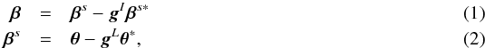$\begin{array}{ccc}{\beta }& \mathrm{=}& {{\beta }}^{\mathit{s}}\mathrm{-}{{g}}^{\mathit{I}}{{\beta }}^{\mathit{s}\mathrm{\ast }}\\ {{\beta }}^{\mathit{s}}& \mathrm{=}& {\theta }\mathrm{-}{{g}}^{\mathit{L}}{{\theta }}^{\mathrm{\ast }}\mathit{,}\end{array}$where g^L is the lensing shear. We set the origin of the coordinates at the centroid of the zero image and the intrinsic image, where the centroid is defined by the condition that the dipole moments of images vanish. The detailed definition can be seen in Okura & Futamase (2014). The combined shear, which is a distortion from the zero plane to the image plane, is written as g, which is given by the lensing shear g^L and the intrinsic shear as follows: 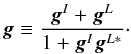$\begin{array}{ccc}{g}\mathrm{\equiv }\frac{{{g}}^{\mathit{I}}\mathrm{+}{{g}}^{\mathit{L}}}{\mathrm{1}\mathrm{+}{{g}}^{\mathit{I}}{{g}}^{\mathit{L}\mathrm{\ast }}}\mathrm{·}& & \end{array}$(3)The intrinsic reduced shear g^I is regarded as a value from intrinsic ellipticity, so it has random orientation. This means the average value of the intrinsic shear tends to 0, so we can estimate lensing shear by averaging Eq. (3).

The complex moments of the measured image are denoted as ${\mathrm{𝒵}}_{\mathit{M}}^{\mathit{N}}$ and measured as 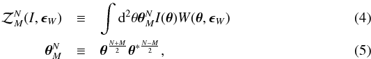$\begin{array}{ccc}{\mathrm{𝒵}}_{\mathit{M}}^{\mathit{N}}\mathrm{\left(}\mathit{I,}{{ϵ}}_{\mathit{W}}\mathrm{\right)}& \mathrm{\equiv }& \int {\mathrm{d}}^{\mathrm{2}}\mathit{\theta }{{\theta }}_{\mathit{M}}^{\mathit{N}}\mathit{I}\mathrm{\left(}{\theta }\mathrm{\right)}\mathit{W}\mathrm{\left(}{\theta }\mathit{,}{{ϵ}}_{\mathit{W}}\mathrm{\right)}\\ {{\theta }}_{\mathit{M}}^{\mathit{N}}& \mathrm{\equiv }& {{\theta }}^{\frac{\mathit{N}\mathrm{+}\mathit{M}}{\mathrm{2}}}{{\theta }}^{\mathrm{\ast }\frac{\mathit{N}\mathrm{-}\mathit{M}}{\mathrm{2}}}\mathit{,}\end{array}$where W is a weight function, which is a function of displacement from the centroid θ and ellipticity ϵ_W. The determination of the ellipticity is explained in the next section and the Appendix, and N is the order of moments and M indicates the spin number. For example: 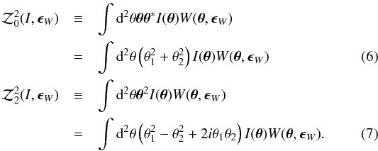$\begin{array}{ccc}{\mathrm{𝒵}}_{\mathrm{0}}^{\mathrm{2}}\mathrm{\left(}\mathit{I,}{{ϵ}}_{\mathit{W}}\mathrm{\right)}& \mathrm{\equiv }& \int {\mathrm{d}}^{\mathrm{2}}\mathit{\theta }{\theta }{{\theta }}^{\mathrm{\ast }}\mathit{I}\mathrm{\left(}{\theta }\mathrm{\right)}\mathit{W}\mathrm{\left(}{\theta }\mathit{,}{{ϵ}}_{\mathit{W}}\mathrm{\right)}\\ & \mathrm{=}& \int {\mathrm{d}}^{\mathrm{2}}\mathit{\theta }\mathrm{(}{\mathit{\theta }}_{\mathrm{1}}^{\mathrm{2}}\mathrm{+}{{\mathit{\theta }}_{\mathrm{2}}^{\mathrm{2}}}^{\mathrm{)}}\mathit{I}\mathrm{\left(}{\theta }\mathrm{\right)}\mathit{W}\mathrm{\left(}{\theta }\mathit{,}{{ϵ}}_{\mathit{W}}\mathrm{\right)}\\ {\mathrm{𝒵}}_{\mathrm{2}}^{\mathrm{2}}\mathrm{\left(}\mathit{I,}{{ϵ}}_{\mathit{W}}\mathrm{\right)}& \mathrm{\equiv }& \int {\mathrm{d}}^{\mathrm{2}}\mathit{\theta }{{\theta }}^{\mathrm{2}}\mathit{I}\mathrm{\left(}{\theta }\mathrm{\right)}\mathit{W}\mathrm{\left(}{\theta }\mathit{,}{{ϵ}}_{\mathit{W}}\mathrm{\right)}\\ & \mathrm{=}& \mathrm{\int }{\mathrm{d}}^{\mathrm{2}}\mathit{\theta }\mathrm{(}{\mathit{\theta }}_{\mathrm{1}}^{\mathrm{2}}\mathrm{-}{\mathit{\theta }}_{\mathrm{2}}^{\mathrm{2}}\mathrm{+}\mathrm{2}\mathit{i}{\mathit{\theta }}_{\mathrm{1}}{\mathit{\theta }}_{\mathrm{2}}\mathrm{)}\mathit{I}\mathrm{\left(}{\theta }\mathrm{\right)}\mathit{W}\mathrm{\left(}{\theta }\mathit{,}{{ϵ}}_{\mathit{W}}\mathrm{\right)}\mathit{.}\end{array}$Thus the usual ellipticity is defined from ${\mathrm{𝒵}}_{\mathrm{2}}^{\mathrm{2}}$ and ${\mathrm{𝒵}}_{\mathrm{0}}^{\mathrm{2}}$. The weight function has an arbitrary profile and size, but it should be chosen to reduce the effect from pixel noise. In the simulation test in this paper, we use an elliptical Gaussian for the weight function.

3. Ellipticity of the 0th order moment

In this section, we define the new ellipticity and its relationship to the usual ellipticity and weak gravitational lensing shear without PSF effect. Weak lensing shear analysis by 0th-ellipticity with PSF correction is explained in Sect. 7.

3.1. Definition

As mentioned in the Introduction, the new ellipticity is defined from the 0th order moments. However, ellipticity must have a property of spin 2, and it seems impossible to derive a spin 2 quantity from monopole moments ${\mathrm{𝒵}}_{\mathrm{0}}^{\mathrm{0}}$. In fact, this is not so. The spin 2 quantity can be constructed as follows. First, we define the 0th order moment that has spin 2 property as 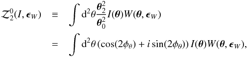$\begin{array}{ccc}{\mathrm{𝒵}}_{\mathrm{2}}^{\mathrm{0}}\mathrm{\left(}\mathit{I,}{{ϵ}}_{\mathit{W}}\mathrm{\right)}& \mathrm{\equiv }& \int {\mathrm{d}}^{\mathrm{2}}\mathit{\theta }\frac{{{\theta }}_{\mathrm{2}}^{\mathrm{2}}}{{{\theta }}_{\mathrm{0}}^{\mathrm{2}}}\mathit{I}\mathrm{\left(}{\theta }\mathrm{\right)}\mathit{W}\mathrm{\left(}{\theta }\mathit{,}{{ϵ}}_{\mathit{W}}\mathrm{\right)}\\ & \mathrm{=}& \mathrm{\int }{\mathrm{d}}^{\mathrm{2}}\mathit{\theta }\left(\cos \mathrm{\left(}\mathrm{2}{\mathit{\phi }}_{\mathit{\theta }}\mathrm{\right)}\mathrm{+}\mathit{i}\sin \mathrm{\left(}\mathrm{2}{\mathit{\phi }}_{\mathit{\theta }}\mathrm{\right)}\right)\mathit{I}\mathrm{\left(}{\theta }\mathrm{\right)}\mathit{W}\mathrm{\left(}{\theta }\mathit{,}{{ϵ}}_{\mathit{W}}\mathrm{\right)}\mathit{,}\end{array}$(8)where φ_θ is the position angle at θ. It has spin 2 nature and thus the ellipticities are defined by normalizing with monopole moments(${\mathrm{𝒵}}_{\mathrm{0}}^{\mathrm{0}}$) to have non-dimension, 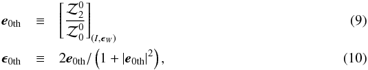$\begin{array}{ccc}{{e}}_{\mathrm{0}\mathrm{th}}& \mathrm{\equiv }& {\left[\frac{{\mathrm{𝒵}}_{\mathrm{2}}^{\mathrm{0}}}{{\mathrm{𝒵}}_{\mathrm{0}}^{\mathrm{0}}}\right]}_{\mathrm{\left(}\mathit{I,}{{ϵ}}_{\mathit{W}}\mathrm{\right)}}\\ {{ϵ}}_{\mathrm{0}\mathrm{th}}& \mathrm{\equiv }& \mathrm{2}{{e}}_{\mathrm{0}\mathrm{th}}\mathit{/}\mathrm{(}\mathrm{1}\mathrm{+}\mathrm{|}{{e}}_{\mathrm{0}\mathrm{th}}{\mathrm{|}}^{\mathrm{2}}\mathrm{)}\mathit{,}\end{array}$where e_0th is the ellipticity measured from 0th order moments and ϵ_0th is another ellipticity used for the ellipticity of the weight function ϵ_W = ϵ_0th in Eq. (8), and the reason for using this ellipticity for weight function is explained in Appendix A. The values of e_0th and ϵ_0th are different, but they provide the same information regarding the ellipticity so they can be transformed into each other.

To distinguish the ellipticities defined by 0th order moments from the ellipticities defined by quadrupole moments, we denote ellipticities defined by quadrupole moments as 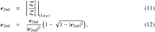$\begin{array}{ccc}{{ϵ}}_{\mathrm{2}\mathrm{nd}}& \mathrm{\equiv }& \left[\frac{{\mathrm{𝒵}}_{\mathrm{2}}^{\mathrm{2}}}{{\mathrm{𝒵}}_{\mathrm{0}}^{\mathrm{2}}}\right]\left(\mathit{I,}{{ϵ}}_{\mathit{W}}\right)\\ {{e}}_{\mathrm{2}\mathrm{nd}}& \mathrm{=}& \frac{{{ϵ}}_{\mathrm{2}\mathrm{nd}}}{\mathrm{|}{{ϵ}}_{\mathrm{2}\mathrm{nd}}{\mathrm{|}}^{\mathrm{2}}}\left(\mathrm{1}\mathrm{-}\sqrt{\mathrm{1}\mathrm{-}\mathrm{|}{{ϵ}}_{\mathrm{2}\mathrm{nd}}{\mathrm{|}}^{\mathrm{2}}}\right)\mathit{,}\end{array}$where the ellipticity of the weight function in Eq. (11) is used and the ellipticity is defined by quadrupole moments, so ϵ_W = ϵ_2nd.

We refer to e_0th and ϵ_0th as the “0th-ellipticity” and e_2nd and ϵ_2nd as the “2nd-ellipticity”. If the profile of the measured image is simple, for example an elliptical Gaussian, the 0th- and 2nd-ellipticities have the same value (e_0th = e_2nd and ϵ_0th = ϵ_2nd), but because a real image has a complex form, these ellipticities usually have different values.

3.2. 0th-ellipticity and reduced shear

Here we present the relationship between the 0th-ellipticity and the reduced shear without the PSF effect. We assume I^Lnsd(θ) to be an image distorted by lensing reduced shear g from the zero image I⁰(β). From the definitions of the 0th-ellipticity, the 0th order moments satisfy the following relationship: $\begin{array}{ccc}{\mathrm{𝒵}}_{\mathrm{2}}^{\mathrm{0}}\mathrm{\left(}{\mathit{I}}^{\mathit{Lnsd}}\mathit{,}{{ϵ}}_{\mathit{W}}\mathrm{\right)}\mathrm{-}{{e}}_{\mathrm{0}\mathrm{th}}{\mathrm{𝒵}}_{\mathrm{0}}^{\mathrm{0}}\mathrm{\left(}{\mathit{I}}^{\mathit{Lnsd}}\mathit{,}{{ϵ}}_{\mathit{W}}\mathrm{\right)}\mathrm{=}\mathrm{0.}& & \end{array}$(13)By transforming Eq. (13) to the zero plane we obtain 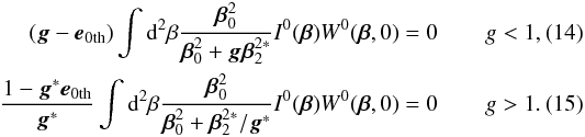$\begin{array}{ccc}\mathrm{(}{g}\mathrm{-}{{e}}_{\mathrm{0}\mathrm{th}}\mathrm{)}\mathrm{\int }{\mathrm{d}}^{\mathrm{2}}\mathit{\beta }\frac{{{\beta }}_{\mathrm{0}}^{\mathrm{2}}}{{{\beta }}_{\mathrm{0}}^{\mathrm{2}}\mathrm{+}{g}{{\beta }}_{\mathrm{2}}^{\mathrm{2}\mathrm{\ast }}}{\mathit{I}}^{\mathrm{0}}\mathrm{\left(}{\beta }\mathrm{\right)}{\mathit{W}}^{\mathrm{0}}\mathrm{\left(}{\beta }\mathit{,}\mathrm{0}\mathrm{\right)}\mathrm{=}\mathrm{0}& & \mathit{g}\mathit{<}\mathrm{1}\mathit{,}\\ \frac{\mathrm{1}\mathrm{-}{{g}}^{\mathrm{\ast }}{{e}}_{\mathrm{0}\mathrm{th}}}{{{g}}^{\mathrm{\ast }}}\mathrm{\int }{\mathrm{d}}^{\mathrm{2}}\mathit{\beta }\frac{{{\beta }}_{\mathrm{0}}^{\mathrm{2}}}{{{\beta }}_{\mathrm{0}}^{\mathrm{2}}\mathrm{+}{{\beta }}_{\mathrm{2}}^{\mathrm{2}\mathrm{\ast }}\mathit{/}{{g}}^{\mathrm{\ast }}}{\mathit{I}}^{\mathrm{0}}\mathrm{\left(}{\beta }\mathrm{\right)}{\mathit{W}}^{\mathrm{0}}\mathrm{\left(}{\beta }\mathit{,}\mathrm{0}\mathrm{\right)}\mathrm{=}\mathrm{0}& & \mathit{g}\mathit{>}\mathrm{1.}\end{array}$Thus, the relationship between the 0th-ellipticity and the reduced shear is obtained as follows: 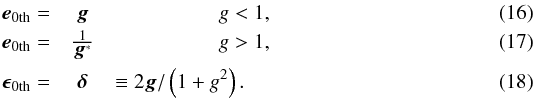$\begin{array}{ccc}{{e}}_{\mathrm{0}\mathrm{th}}\mathrm{=}& {g}& \mathit{g}\mathit{<}\mathrm{1}\mathit{,}\\ {{e}}_{\mathrm{0}\mathrm{th}}\mathrm{=}& \frac{\mathrm{1}}{{{g}}^{\mathrm{\ast }}}& \mathit{g}\mathit{>}\mathrm{1}\mathit{,}\\ {{ϵ}}_{\mathrm{0}\mathrm{th}}\mathrm{=}& {\delta }& \mathrm{\equiv }\mathrm{2}{g}\mathit{/}\mathrm{(}\mathrm{1}\mathrm{+}{\mathit{g}}^{\mathrm{2}}\mathrm{)}\mathit{.}\end{array}$Detailed calculations are shown in Appendix A. This result shows that the reduced shear can be obtained from the 0th-ellipticity. At the same time, the reduced shear can also be obtained from the 2nd-ellipticity. Since the 2nd-ellipticity is induced by the same lensing effect, more accurate weak lensing analysis will be achieved by combining these two ellipticities simultaneously.

4. Effective signal-to-noise ratio

In this section, we show improvement of the S/N in the measurement of the 0th-ellipticity compared with the 2nd-ellipticity.

The regions for measuring the monopole (quadrupole) moment and 0th (2nd)-ellipticity are the same. Therefore the S/N of the 0th (2nd)-ellipticity SN_0th(SN_2nd) is the same as that of the monopole(quadrupole) moments.

Usually the S/N is defined as 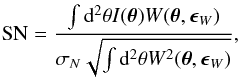$\begin{array}{ccc}\mathrm{SN}\mathrm{=}\frac{\mathrm{\int }{\mathrm{d}}^{\mathrm{2}}\mathit{\theta I}\mathrm{\left(}{\theta }\mathrm{\right)}\mathit{W}\mathrm{\left(}{\theta }\mathit{,}{{ϵ}}_{\mathit{W}}\mathrm{\right)}}{{\mathit{\sigma }}_{\mathit{N}}\sqrt{\mathrm{\int }{\mathrm{d}}^{\mathrm{2}}\mathit{\theta }{\mathit{W}}^{\mathrm{2}}\mathrm{\left(}{\theta }\mathit{,}{{ϵ}}_{\mathit{W}}\mathrm{\right)}}}\mathit{,}& & \end{array}$(19)where σ_N is the standard deviation of pixel noise, and therefore this is also the S/N of the monopole moment. Thus we obtain SN_0th = SN. However, the quadrupole moment has a different S/N from that of the monopole moment, because the region used to measure the monopole and quadrupole moments are different. Therefore, the quadrupole moment and 2nd-ellipticity have different signal and noise from SN_0th, and is defined as 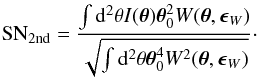$\begin{array}{ccc}{\mathrm{SN}}_{\mathrm{2}\mathrm{nd}}\mathrm{=}\frac{\mathrm{\int }{\mathrm{d}}^{\mathrm{2}}\mathit{\theta I}\mathrm{\left(}{\theta }\mathrm{\right)}{{\theta }}_{\mathrm{0}}^{\mathrm{2}}\mathit{W}\mathrm{\left(}{\theta }\mathit{,}{{ϵ}}_{\mathit{W}}\mathrm{\right)}}{\sqrt{\mathrm{\int }{\mathrm{d}}^{\mathrm{2}}\mathit{\theta }{{\theta }}_{\mathrm{0}}^{\mathrm{4}}{\mathit{W}}^{\mathrm{2}}\mathrm{\left(}{\theta }\mathit{,}{{ϵ}}_{\mathit{W}}\mathrm{\right)}}}\mathrm{·}& & \end{array}$(20)Now we consider an image which has a Gaussian brightness distribution to analytically compare these S/Ns. The ratio of the S/Ns for a Gaussian image with the same weight function is given by 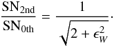$\begin{array}{ccc}\frac{{\mathrm{SN}}_{\mathrm{2}\mathrm{nd}}}{{\mathrm{SN}}_{\mathrm{0}\mathrm{th}}}\mathrm{=}\frac{\mathrm{1}}{\sqrt{\mathrm{2}\mathrm{+}{\mathit{ϵ}}_{\mathit{W}}^{\mathrm{2}}}}\mathrm{·}& & \end{array}$(21)This result means that the S/N of the quadrupole moment is lower than that of the monopole moment on the order of $\sqrt{\mathrm{2}}\mathrm{~}\sqrt{\mathrm{3}}$ because the monopole moment is measured in the central (brighter) region. Therefore, it is expected that the reduced shear can be measured by using the 0th-ellipticity with a higher S/N compared to using the 2nd-ellipticity. We measured the S/N with real data in Sect. 6.

5. Integration problem

In this section, we present a problem and a correction in measuring moments by integration of the 0th-ellipticity, which is distinct from the sampling or pixelization problem considered in typical image analysis.

Moments are defined by integration of the image count and some functions of distance from the centroid, e.g. Eq. (4). However, in the analysis of actual data, we do not use integration to measure the moments, because the image is observed by CCD pixels. Thus, instead of the integration, we use a sum of sampling counted CCD pixels, and Eq. (8) becomes $\begin{array}{ccc}{\mathrm{𝒵}}_{\mathrm{2}}^{\mathrm{0}}\mathrm{\left(}\mathit{I,}{{ϵ}}_{\mathit{W}}\mathrm{\right)}& \mathrm{=}& \sum _{\mathit{x}}\sum _{\mathit{y}}\frac{{{{\theta }}_{\mathit{xy}}}_{\mathrm{2}}^{\mathrm{2}}}{{{{\theta }}_{\mathit{xy}}}_{\mathrm{0}}^{\mathrm{2}}}\mathit{I}\mathrm{\left(}{{\theta }}_{\mathit{xy}}\mathrm{\right)}\mathit{W}\mathrm{\left(}{{\theta }}_{\mathit{xy}}\mathit{,}{{ϵ}}_{\mathit{W}}\mathrm{\right)}\\ & \mathrm{=}& \sum _{\mathit{x}}\sum _{\mathit{y}}\mathrm{(}\cos \mathrm{(}\mathrm{2}{\mathit{\phi }}_{\mathit{\theta xy}}\mathrm{+}\mathit{i}\sin \mathrm{(}\mathrm{2}{\mathit{\phi }}_{\mathit{\theta xy}}{\mathrm{)}}^{\mathrm{)}}\mathit{I}\mathrm{\left(}{{\theta }}_{\mathit{xy}}\mathrm{\right)}\mathit{W}\mathrm{\left(}{{\theta }}_{\mathit{ixy}}\mathit{,}{{ϵ}}_{\mathit{W}}\mathrm{\right)}\mathit{,}\end{array}$(22)where θ_xy = θ_x + iθ_y is the displacement of position in the bottom left corner of each pixel from the centroid. However, ${{{\theta }}_{\mathit{xy}}}_{\mathrm{2}}^{\mathrm{2}}\mathit{/}{{{\theta }}_{\mathit{xy}}}_{\mathrm{0}}^{\mathrm{2}}$ changes violently in a pixel, especially if the CCD pixels are near the centroid, then the sampling count in Eq. (22) makes an incorrect count for the moment. In measuring the quadrupole moments, this effect is sufficiently small, because ${{{\theta }}_{\mathit{xy}}}_{\mathrm{2}}^{\mathrm{2}}$ takes almost 0 at pixels near the centroid. To correct this effect, we use integration only for ${{{\theta }}_{\mathit{xy}}}_{\mathrm{2}}^{\mathrm{2}}\mathit{/}{{{\theta }}_{\mathit{xy}}}_{\mathrm{0}}^{\mathrm{2}}$ and Eq. (22) is redefined as 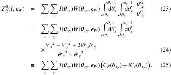$\begin{array}{ccc}{\mathrm{𝒵}}_{\mathrm{2}}^{\mathrm{0}}\mathrm{\left(}\mathit{I,}{{ϵ}}_{\mathit{W}}\mathrm{\right)}& \mathrm{=}& \sum _{\mathit{x}}\sum _{\mathit{y}}\mathit{I}\mathrm{\left(}{{\theta }}_{\mathit{xy}}\mathrm{\right)}\mathit{W}\mathrm{\left(}{{\theta }}_{\mathit{xy}}\mathit{,}{{ϵ}}_{\mathit{W}}\mathrm{\right)}{\mathrm{\int }}_{{\mathit{\theta }}_{\mathit{x}}}^{{\mathit{\theta }}_{\mathit{x}}\mathrm{+}\mathrm{1}}\mathrm{d}{\mathit{\theta }}_{\mathit{x}}^{\mathrm{\prime }}{\mathrm{\int }}_{{\mathit{\theta }}_{\mathit{y}}}^{{\mathit{\theta }}_{\mathit{y}}\mathrm{+}\mathrm{1}}\mathrm{d}{\mathit{\theta }}_{\mathit{y}}^{\mathrm{\prime }}\frac{{{{\theta }}^{\mathrm{\prime }}}_{\mathrm{2}}^{\mathrm{2}}}{{{{\theta }}^{\mathrm{\prime }}}_{\mathrm{0}}^{\mathrm{2}}}\\ & \mathrm{=}& \sum _{\mathit{x}}\sum _{\mathit{y}}\mathit{I}\mathrm{\left(}{{\theta }}_{\mathit{xy}}\mathrm{\right)}\mathit{W}\mathrm{\left(}{{\theta }}_{\mathit{xy}}\mathit{,}{{ϵ}}_{\mathit{W}}\mathrm{\right)}{\mathrm{\int }}_{{\mathit{\theta }}_{\mathit{x}}}^{{\mathit{\theta }}_{\mathit{x}}\mathrm{+}\mathrm{1}}\mathrm{d}{\mathit{\theta }}_{\mathit{x}}^{\mathrm{\prime }}{\mathrm{\int }}_{{\mathit{\theta }}_{\mathit{y}}}^{{\mathit{\theta }}_{\mathit{y}}\mathrm{+}\mathrm{1}}\mathrm{d}{\mathit{\theta }}_{\mathit{y}}^{\mathrm{\prime }}\\ & & \mathrm{\times }\frac{{{{\mathit{\theta }}^{\mathrm{\prime }}}_{\mathit{x}}}^{\mathrm{2}}\mathrm{-}{{{\mathit{\theta }}^{\mathrm{\prime }}}_{\mathit{y}}}^{\mathrm{2}}\mathrm{+}\mathrm{2}\mathit{i}{{\mathit{\theta }}^{\mathrm{\prime }}}_{\mathit{x}}{{\mathit{\theta }}^{\mathrm{\prime }}}_{\mathit{y}}}{{{{\mathit{\theta }}^{\mathrm{\prime }}}_{\mathit{x}}}^{\mathrm{2}}\mathrm{+}{{{\mathit{\theta }}^{\mathrm{\prime }}}_{\mathit{y}}}^{\mathrm{2}}}\\ & \mathrm{\equiv }& \sum _{\mathit{x}}\sum _{\mathit{y}}\mathit{I}\mathrm{\left(}{{\theta }}_{\mathit{xy}}\mathrm{\right)}\mathit{W}\mathrm{\left(}{{\theta }}_{\mathit{xy}}\mathit{,}{{ϵ}}_{\mathit{W}}\mathrm{\right)}\mathrm{(}{\mathit{C}}_{\mathit{R}}\mathrm{\left(}{{\theta }}_{\mathit{xy}}\mathrm{\right)}\mathrm{+}\mathit{i}{\mathit{C}}_{\mathit{I}}\mathrm{(}{{\theta }}_{\mathit{xy}}{\mathrm{)}}^{\mathrm{)}}\mathit{.} \end{array}$This integration can be calculated analytically as $\begin{array}{ccc}{\mathrm{\int }}_{{\mathit{\theta }}_{\mathit{x}}}^{{\mathit{\theta }}_{\mathit{x}}\mathrm{+}\mathrm{1}}\mathrm{d}{\mathit{\theta }}_{\mathit{x}}^{\mathrm{\prime }}{\mathrm{\int }}_{{\mathit{\theta }}_{\mathit{y}}}^{{\mathit{\theta }}_{\mathit{y}}\mathrm{+}\mathrm{1}}\mathrm{d}{\mathit{\theta }}_{\mathit{y}}^{\mathrm{\prime }}\frac{{{{\mathit{\theta }}^{\mathrm{\prime }}}_{\mathit{x}}}^{\mathrm{2}}\mathrm{-}{{{\mathit{\theta }}^{\mathrm{\prime }}}_{\mathit{y}}}^{\mathrm{2}}}{{{{\mathit{\theta }}^{\mathrm{\prime }}}_{\mathit{x}}}^{\mathrm{2}}\mathrm{+}{{{\mathit{\theta }}^{\mathrm{\prime }}}_{\mathit{y}}}^{\mathrm{2}}}\mathrm{=}& & \\ & & [\left[\mathrm{(}{{\mathit{\theta }}^{\mathrm{\prime }}}_{\mathit{x}}^{\mathrm{2}}\mathrm{+}{{{\mathit{\theta }}^{\mathrm{\prime }}}_{\mathit{y}}^{\mathrm{2}}}^{\mathrm{)}}{\tan }^{-1}\left(\frac{{{\mathit{\theta }}^{\mathrm{\prime }}}_{\mathit{y}}}{{{\mathit{\theta }}^{\mathrm{\prime }}}_{\mathit{x}}}\right)\right]\begin{array}{c}{\mathit{\theta }}_{\mathit{x}}\mathrm{+}\mathrm{1}\\ {\mathit{\theta }}_{\mathit{x}}\end{array}{]}_{{\mathit{\theta }}_{\mathit{y}}}^{{\mathit{\theta }}_{\mathit{y}}\mathrm{+}\mathrm{1}}{{\mathit{\theta }}^{\mathrm{\prime }}}_{\mathit{x}}\ne \mathrm{0} \\ & \mathrm{\equiv }& [{\mathrm{[}{\mathit{F}}_{\mathrm{A}}\mathrm{(}{\mathit{\theta }}_{\mathit{x}}\mathit{,}{\mathit{\theta }}_{\mathit{y}}{\mathrm{)}}^{\mathrm{]}}}_{{\mathit{\theta }}_{\mathit{x}}}^{{\mathit{\theta }}_{\mathit{x}}\mathrm{+}\mathrm{1}}{]}_{{\mathit{\theta }}_{\mathit{y}}}^{{\mathit{\theta }}_{\mathit{y}}\mathrm{+}\mathrm{1}}{{\mathit{\theta }}^{\mathrm{\prime }}}_{\mathit{x}}\ne \mathrm{0} \\ {\mathrm{\int }}_{{\mathit{\theta }}_{\mathit{x}}}^{{\mathit{\theta }}_{\mathit{x}}\mathrm{+}\mathrm{1}}\mathrm{d}{\mathit{\theta }}_{\mathit{x}}^{\mathrm{\prime }}{\mathrm{\int }}_{{\mathit{\theta }}_{\mathit{y}}}^{{\mathit{\theta }}_{\mathit{y}}\mathrm{+}\mathrm{1}}\mathrm{d}{\mathit{\theta }}_{\mathit{y}}^{\mathrm{\prime }}\frac{{{{\mathit{\theta }}^{\mathrm{\prime }}}_{\mathit{x}}}^{\mathrm{2}}\mathrm{-}{{{\mathit{\theta }}^{\mathrm{\prime }}}_{\mathit{y}}}^{\mathrm{2}}}{{{{\mathit{\theta }}^{\mathrm{\prime }}}_{\mathit{x}}}^{\mathrm{2}}\mathrm{+}{{{\mathit{\theta }}^{\mathrm{\prime }}}_{\mathit{y}}}^{\mathrm{2}}}& & \\ & \mathrm{=}& \mathrm{-}[\left[\mathrm{(}{{\mathit{\theta }}^{\mathrm{\prime }}}_{\mathit{x}}^{\mathrm{2}}\mathrm{+}{{{\mathit{\theta }}^{\mathrm{\prime }}}_{\mathit{y}}^{\mathrm{2}}}^{\mathrm{)}}{\tan }^{-1}\left(\frac{{{\mathit{\theta }}^{\mathrm{\prime }}}_{\mathit{x}}}{{{\mathit{\theta }}^{\mathrm{\prime }}}_{\mathit{y}}}\right)\right]\begin{array}{c}{\mathit{\theta }}_{\mathit{x}}\mathrm{+}\mathrm{1}\\ {\mathit{\theta }}_{\mathit{x}}\end{array}{]}_{{\mathit{\theta }}_{\mathit{y}}}^{{\mathit{\theta }}_{\mathit{y}}\mathrm{+}\mathrm{1}}{{\mathit{\theta }}^{\mathrm{\prime }}}_{\mathit{y}}\ne \mathrm{0} \\ & \mathrm{=}& [{\mathrm{[}{\mathit{F}}_{\mathrm{B}}\mathrm{(}{\mathit{\theta }}_{\mathit{x}}\mathit{,}{\mathit{\theta }}_{\mathit{y}}{\mathrm{)}}^{\mathrm{]}}}_{{\mathit{\theta }}_{\mathit{x}}}^{{\mathit{\theta }}_{\mathit{x}}\mathrm{+}\mathrm{1}}{]}_{{\mathit{\theta }}_{\mathit{y}}}^{{\mathit{\theta }}_{\mathit{y}}\mathrm{+}\mathrm{1}}{{\mathit{\theta }}^{\mathrm{\prime }}}_{\mathit{y}}\ne \mathrm{0} \end{array}$\newpage

$\begin{array}{ccc}{\mathrm{\int }}_{{\mathit{\theta }}_{\mathit{x}}}^{{\mathit{\theta }}_{\mathit{x}}\mathrm{+}\mathrm{1}}\mathrm{d}{\mathit{\theta }}_{\mathit{x}}^{\mathrm{\prime }}{\mathrm{\int }}_{{\mathit{\theta }}_{\mathit{y}}}^{{\mathit{\theta }}_{\mathit{y}}\mathrm{+}\mathrm{1}}\mathrm{d}{\mathit{\theta }}_{\mathit{y}}^{\mathrm{\prime }}\frac{\mathrm{2}{{\mathit{\theta }}^{\mathrm{\prime }}}_{\mathit{x}}{{\mathit{\theta }}^{\mathrm{\prime }}}_{\mathit{y}}}{{{{\mathit{\theta }}^{\mathrm{\prime }}}_{\mathit{x}}}^{\mathrm{2}}\mathrm{+}{{{\mathit{\theta }}^{\mathrm{\prime }}}_{\mathit{y}}}^{\mathrm{2}}}& & \\ & \mathrm{=}& \frac{\mathrm{1}}{\mathrm{2}}[{\mathrm{[}\mathrm{(}{{\mathit{\theta }}^{\mathrm{\prime }}}_{\mathit{x}}^{\mathrm{2}}\mathrm{+}{{{\mathit{\theta }}^{\mathrm{\prime }}}_{\mathit{y}}^{\mathrm{2}}}^{\mathrm{)}}\log {\mathrm{(}{{{\mathit{\theta }}^{\mathrm{\prime }}}_{\mathit{x}}}^{\mathrm{2}}\mathrm{+}{{{\mathit{\theta }}^{\mathrm{\prime }}}_{\mathit{y}}}^{\mathrm{2}}\mathrm{)}}^{\mathrm{]}}}_{{\mathit{\theta }}_{\mathit{x}}}^{{\mathit{\theta }}_{\mathit{x}}\mathrm{+}\mathrm{1}}{]}_{{\mathit{\theta }}_{\mathit{y}}}^{{\mathit{\theta }}_{\mathit{y}}\mathrm{+}\mathrm{1}}\\ & \mathrm{\equiv }& \frac{\mathrm{1}}{\mathrm{2}}[{\mathrm{[}{\mathit{F}}_{\mathit{C}}\mathrm{(}{\mathit{\theta }}_{\mathit{x}}\mathit{,}{\mathit{\theta }}_{\mathit{y}}{\mathrm{)}}^{\mathrm{]}}}_{{\mathit{\theta }}_{\mathit{x}}}^{{\mathit{\theta }}_{\mathit{x}}\mathrm{+}\mathrm{1}}{]}_{{\mathit{\theta }}_{\mathit{y}}}^{{\mathit{\theta }}_{\mathit{y}}\mathrm{+}\mathrm{1}}\mathrm{;}\end{array}$therefore, we can obtain C_R and C_I analytically as $\begin{array}{ccc}{\mathit{C}}_{\mathit{R}}\mathrm{\left(}{{\theta }}_{\mathit{xy}}\mathrm{\right)}& & \\ & \mathrm{=}& [{\mathrm{[}{\mathit{F}}_{\mathrm{A}}\mathrm{(}{\mathit{\theta }}_{\mathit{x}}\mathit{,}{\mathit{\theta }}_{\mathit{y}}{\mathrm{)}}^{\mathrm{]}}}_{{\mathit{\theta }}_{\mathit{x}}}^{{\mathit{\theta }}_{\mathit{x}}\mathrm{+}\mathrm{1}}{]}_{{\mathit{\theta }}_{\mathit{y}}}^{{\mathit{\theta }}_{\mathit{y}}\mathrm{+}\mathrm{1}}\mathrm{if}\mathrm{|}{\mathit{\theta }}_{\mathit{x}}\mathrm{+}\mathrm{0.5}\mathrm{|}\mathit{>}\mathrm{|}{\mathit{\theta }}_{\mathit{y}}\mathrm{+}\mathrm{0.5}\mathrm{|}\mathit{,} \\ {\mathit{C}}_{\mathit{R}}\mathrm{\left(}{{\theta }}_{\mathit{xy}}\mathrm{\right)}& & \\ & \mathrm{=}& [{\mathrm{[}{\mathit{F}}_{\mathrm{B}}\mathrm{(}{\mathit{\theta }}_{\mathit{x}}\mathit{,}{\mathit{\theta }}_{\mathit{y}}{\mathrm{)}}^{\mathrm{]}}}_{{\mathit{\theta }}_{\mathit{x}}}^{{\mathit{\theta }}_{\mathit{x}}\mathrm{+}\mathrm{1}}{]}_{{\mathit{\theta }}_{\mathit{y}}}^{{\mathit{\theta }}_{\mathit{y}}\mathrm{+}\mathrm{1}}\mathrm{if}\mathrm{|}{\mathit{\theta }}_{\mathit{y}}\mathrm{+}\mathrm{0.5}\mathrm{|}\mathit{>}\mathrm{|}{\mathit{\theta }}_{\mathit{x}}\mathrm{+}\mathrm{0.5}\mathrm{|} \\ {\mathit{C}}_{\mathit{R}}\mathrm{\left(}{{\theta }}_{\mathit{xy}}\mathrm{\right)}& & \\ & \mathrm{=}& \frac{\mathrm{1}}{\mathrm{2}}([{\mathrm{[}{\mathit{F}}_{\mathrm{A}}\mathrm{(}{\mathit{\theta }}_{\mathit{x}}\mathit{,}{\mathit{\theta }}_{\mathit{y}}{\mathrm{)}}^{\mathrm{]}}}_{{\mathit{\theta }}_{\mathit{x}}}^{{\mathit{\theta }}_{\mathit{x}}\mathrm{+}\mathrm{1}}{]}_{{\mathit{\theta }}_{\mathit{y}}}^{{\mathit{\theta }}_{\mathit{y}}\mathrm{+}\mathrm{1}}\mathrm{+}[{\mathrm{[}{\mathit{F}}_{\mathrm{B}}\mathrm{(}{\mathit{\theta }}_{\mathit{x}}\mathit{,}{\mathit{\theta }}_{\mathit{y}}{\mathrm{)}}^{\mathrm{]}}}_{{\mathit{\theta }}_{\mathit{x}}}^{{\mathit{\theta }}_{\mathit{x}}\mathrm{+}\mathrm{1}}{]}_{{\mathit{\theta }}_{\mathit{y}}}^{{\mathit{\theta }}_{\mathit{y}}\mathrm{+}\mathrm{1}}\\ & & \mathrm{+}\mathit{\pi }\left(\frac{{\mathrm{(}{\mathit{\theta }}_{\mathit{x}}\mathrm{+}{\mathrm{1}}^{\mathrm{)}}}^{\mathrm{3}}}{\mathrm{|}{\mathit{\theta }}_{\mathit{x}}\mathrm{+}\mathrm{1}\mathrm{|}}\mathrm{-}\frac{{\mathrm{(}{\mathit{\theta }}_{\mathit{x}}\mathrm{)}}^{\mathrm{3}}}{\mathrm{\left|}{\mathit{\theta }}_{\mathit{x}}\mathrm{\right|}}\mathrm{-}\frac{{\mathrm{(}{\mathit{\theta }}_{\mathit{y}}\mathrm{+}{\mathrm{1}}^{\mathrm{)}}}^{\mathrm{3}}}{\mathrm{|}{\mathit{\theta }}_{\mathit{y}}\mathrm{+}\mathrm{1}\mathrm{|}}\mathrm{+}\frac{{\mathrm{(}{\mathit{\theta }}_{\mathit{y}}\mathrm{)}}^{\mathrm{3}}}{\mathrm{\left|}{\mathit{\theta }}_{\mathit{y}}\mathrm{\right|}}\right))\\ & & \mathrm{if}\mathrm{(}\mathrm{-}\mathrm{1}\mathit{<}{\mathit{\theta }}_{\mathit{x}}\mathit{<}\mathrm{0}\mathrm{)}\mathrm{and}\mathrm{(}\mathrm{-}\mathrm{1}\mathit{<}{\mathit{\theta }}_{\mathit{y}}\mathit{<}\mathrm{0}\mathrm{)}\\ {\mathit{C}}_{\mathit{I}}\mathrm{\left(}{{\theta }}_{\mathit{xy}}\mathrm{\right)}& \mathrm{=}& \frac{\mathrm{1}}{\mathrm{2}}[{\mathrm{[}{\mathit{F}}_{\mathit{C}}\mathrm{(}{\mathit{\theta }}_{\mathit{x}}\mathit{,}{\mathit{\theta }}_{\mathit{y}}{\mathrm{)}}^{\mathrm{]}}}_{{\mathit{\theta }}_{\mathit{x}}}^{{\mathit{\theta }}_{\mathit{x}}\mathrm{+}\mathrm{1}}{]}_{{\mathit{\theta }}_{\mathit{y}}}^{{\mathit{\theta }}_{\mathit{y}}\mathrm{+}\mathrm{1}}\mathit{,}\end{array}$where Eq. (34) is a formula about integration in the pixel, which is the centre of image. This formula can be derived as $\begin{array}{ccc}{\mathit{C}}_{\mathit{R}}\mathrm{\left(}{{\theta }}_{\mathit{xy}}\mathrm{\right)}& & \\ & \mathrm{=}& \frac{\mathrm{1}}{\mathrm{2}}\underset{\mathit{\delta }\mathrm{\to }\mathrm{0}}{\lim }([{\mathrm{[}{\mathit{F}}_{\mathrm{A}}\mathrm{(}{\mathit{\theta }}_{\mathit{x}}\mathit{,}{\mathit{\theta }}_{\mathit{y}}{\mathrm{)}}^{\mathrm{]}}}_{{\mathit{\theta }}_{\mathit{x}}}^{\mathrm{-}\mathit{\delta }}\mathrm{+}{\mathrm{[}{\mathit{F}}_{\mathrm{A}}\mathrm{(}{\mathit{\theta }}_{\mathit{x}}\mathit{,}{\mathit{\theta }}_{\mathit{y}}{\mathrm{)}}^{\mathrm{]}}}_{\mathit{\delta }}^{{\mathit{\theta }}_{\mathit{x}}\mathrm{+}\mathrm{1}}{]}_{{\mathit{\theta }}_{\mathit{y}}}^{{\mathit{\theta }}_{\mathit{y}}\mathrm{+}\mathrm{1}}\\ & & \mathrm{+}[{\mathrm{[}{\mathit{F}}_{\mathrm{B}}\mathrm{(}{\mathit{\theta }}_{\mathit{x}}\mathit{,}{\mathit{\theta }}_{\mathit{y}}{\mathrm{)}}^{\mathrm{]}}}_{{\mathit{\theta }}_{\mathit{y}}}^{\mathrm{-}\mathit{\delta }}\mathrm{+}{\mathrm{[}{\mathit{F}}_{\mathrm{B}}\mathrm{(}{\mathit{\theta }}_{\mathit{x}}\mathit{,}{\mathit{\theta }}_{\mathit{y}}{\mathrm{)}}^{\mathrm{]}}}_{\mathit{\delta }}^{{\mathit{\theta }}_{\mathit{y}}\mathrm{+}\mathrm{1}}{]}_{{\mathit{\theta }}_{\mathit{x}}}^{{\mathit{\theta }}_{\mathit{x}}\mathrm{+}\mathrm{1}})\\ & \mathrm{=}& \frac{\mathrm{1}}{\mathrm{2}}([{\mathrm{[}{\mathit{F}}_{\mathrm{A}}\mathrm{\left(}{\mathit{\theta }}_{\mathit{x}}\mathit{,}{\mathit{\theta }}_{\mathit{y}}\mathrm{\right)}\mathrm{+}{\mathit{F}}_{\mathrm{B}}\mathrm{(}{\mathit{\theta }}_{\mathit{x}}\mathit{,}{\mathit{\theta }}_{\mathit{y}}{\mathrm{)}}^{\mathrm{]}}}_{{\mathit{\theta }}_{\mathit{y}}}^{{\mathit{\theta }}_{\mathit{y}}\mathrm{+}\mathrm{1}}{]}_{{\mathit{\theta }}_{\mathit{x}}}^{{\mathit{\theta }}_{\mathit{x}}\mathrm{+}\mathrm{1}}\\ & & \mathrm{+}\underset{\mathit{\delta }\mathrm{\to }\mathrm{0}}{\lim }(\mathrm{-}{\mathrm{(}{\mathit{\theta }}_{\mathit{y}}\mathrm{+}{\mathrm{1}}^{\mathrm{)}}}^{\mathrm{2}}\arctan \left(\frac{{\mathit{\theta }}_{\mathit{y}}\mathrm{+}\mathrm{1}}{\mathit{\delta }}\right)\mathrm{+}{\mathrm{(}{\mathit{\theta }}_{\mathit{y}}\mathrm{+}{\mathrm{1}}^{\mathrm{)}}}^{\mathrm{2}}\arctan \left(\mathrm{-}\frac{{\mathit{\theta }}_{\mathit{y}}\mathrm{+}\mathrm{1}}{\mathit{\delta }}\right)\\ & & \mathrm{+}{\mathrm{(}{\mathit{\theta }}_{\mathit{y}}\mathrm{)}}^{\mathrm{2}}\arctan \left(\frac{{\mathit{\theta }}_{\mathit{y}}}{\mathit{\delta }}\right)\mathrm{-}{\mathrm{(}{\mathit{\theta }}_{\mathit{y}}\mathrm{)}}^{\mathrm{2}}\arctan \left(\mathrm{-}\frac{{\mathit{\theta }}_{\mathit{y}}}{\mathit{\delta }}\right)\\ & & \mathrm{+}{\mathrm{(}{\mathit{\theta }}_{\mathit{x}}\mathrm{+}{\mathrm{1}}^{\mathrm{)}}}^{\mathrm{2}}\arctan \left(\frac{{\mathit{\theta }}_{\mathit{x}}\mathrm{+}\mathrm{1}}{\mathit{\delta }}\right)\mathrm{-}{\mathrm{(}{\mathit{\theta }}_{\mathit{x}}\mathrm{+}{\mathrm{1}}^{\mathrm{)}}}^{\mathrm{2}}\arctan \left(\mathrm{-}\frac{{\mathit{\theta }}_{\mathit{x}}\mathrm{+}\mathrm{1}}{\mathit{\delta }}\right)\\ & & \mathrm{-}{\mathrm{(}{\mathit{\theta }}_{\mathit{x}}\mathrm{)}}^{\mathrm{2}}\arctan \left(\frac{{\mathit{\theta }}_{\mathit{x}}}{\mathit{\delta }}\right)\mathrm{+}{\mathrm{(}{\mathit{\theta }}_{\mathit{x}}\mathrm{)}}^{\mathrm{2}}\arctan \left(\mathrm{-}\frac{{\mathit{\theta }}_{\mathit{x}}}{\mathit{\delta }}\right)))\\ & \mathrm{=}& \frac{\mathrm{1}}{\mathrm{2}}([{\mathrm{[}{\mathit{F}}_{\mathrm{A}}\mathrm{\left(}{\mathit{\theta }}_{\mathit{x}}\mathit{,}{\mathit{\theta }}_{\mathit{y}}\mathrm{\right)}\mathrm{+}{\mathit{F}}_{\mathrm{B}}\mathrm{(}{\mathit{\theta }}_{\mathit{x}}\mathit{,}{\mathit{\theta }}_{\mathit{y}}{\mathrm{)}}^{\mathrm{]}}}_{{\mathit{\theta }}_{\mathit{y}}}^{{\mathit{\theta }}_{\mathit{y}}\mathrm{+}\mathrm{1}}{]}_{{\mathit{\theta }}_{\mathit{x}}}^{{\mathit{\theta }}_{\mathit{x}}\mathrm{+}\mathrm{1}}\\ & & \mathrm{+}\mathit{\pi }\left(\frac{{\mathrm{(}{\mathit{\theta }}_{\mathit{x}}\mathrm{+}{\mathrm{1}}^{\mathrm{)}}}^{\mathrm{3}}}{\mathrm{|}{\mathit{\theta }}_{\mathit{x}}\mathrm{+}\mathrm{1}\mathrm{|}}\mathrm{-}\frac{{\mathrm{(}{\mathit{\theta }}_{\mathit{x}}\mathrm{)}}^{\mathrm{3}}}{\mathrm{\left|}{\mathit{\theta }}_{\mathit{x}}\mathrm{\right|}}\mathrm{-}\frac{{\mathrm{(}{\mathit{\theta }}_{\mathit{y}}\mathrm{+}{\mathrm{1}}^{\mathrm{)}}}^{\mathrm{3}}}{\mathrm{|}{\mathit{\theta }}_{\mathit{y}}\mathrm{+}\mathrm{1}\mathrm{|}}\mathrm{+}\frac{{\mathrm{(}{\mathit{\theta }}_{\mathit{y}}\mathrm{)}}^{\mathrm{3}}}{\mathrm{\left|}{\mathit{\theta }}_{\mathit{y}}\mathrm{\right|}}\right))\mathrm{·}\end{array}$(36)

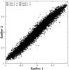Fig. 1 Correlation between 0th- and 2nd-epsilon values measured from real data.

6. Statistics obtained from real data

In this section, we show the statistics of the ellipticities and S/Ns obtained using data from Abell 1689.

6.1. Data

We used real data from the field of Abell 1689, which was observed by the Subaru telescope and Suprime-Cam. Objects were detected by Sextractor and we selected objects that are larger than stars. The region of the data is about 0.245(deg²) and the number of the selected background objects is 22 302 (~25/arcmin²).

6.2. Statistics

We now present the statistics of the ellipticities and the S/Ns for the selected objects. Figure 1 shows the correlation between the 0th- and 2nd-ellipticites, where the 0th-ellipticities are plotted on the horizontal axis and the 2nd-ellipticities are on the vertical axis. A cut-off for objects that have | ϵ_2nd | > 0.9 was used. The figure shows a high correlation, and thus we can equally use the 0th-ellipticity as a tool for weak shear measurement in the analysis of real data.

The upper part of Fig. 2 shows the relationship between the ellipticity and the ratio between SN_0th and SN_2nd, where | ϵ_0th | is plotted on the horizontal axis and the ratio SN_0th/ SN_2nd is on the vertical axis. The dashed line in the figure is $\sqrt{\mathrm{2}\mathrm{+}\mathrm{|}{{ϵ}}_{\mathrm{0}\mathrm{th}}{\mathrm{|}}^{\mathrm{2}}}$, which is the predicted function for an elliptical Gaussian image. The bottom part of Fig. 2 shows the difference in the S/N from $\sqrt{\mathrm{2}\mathrm{+}\mathrm{|}{{ϵ}}_{\mathrm{0}\mathrm{th}}{\mathrm{|}}^{\mathrm{2}}}$. These figures show that the prediction is a good approximation for real objects. The values of SN_0th for real objects are $\sqrt{\mathrm{2}}\mathrm{~}\sqrt{\mathrm{3}}\mathrm{(}\mathrm{~}\mathrm{1.5}\mathrm{)}$ times larger than SN_2nd. Figures 3 and 4 show the distributions of the number count for each of the S/N bins. It can be seen that the number count of SN_0th is distributed in higher S/N bins than that of SN_2nd, which is consistent with Fig. 2. Based on the above measurements, the 0th-ellipticity has a 1.5 times larger S/N than that of the 2nd-ellipticity, which means that the lower limit of the S/N can be set to a 1.5 times smaller value for the 0th-ellipticity with the same precision of pixel noise. Therefore, it is expected that the available number of background objects will increase, and as a result, the statistical error in the weak lensing shear measurement scheme is lower than with the previous method. A more detailed and qualitative study of error estimation will be given in a forthcoming paper.

Fig. 2 Epsilon vs. S/N measured from real data.

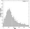Fig. 3 Distribution of the normalized number count of S/N monopole.

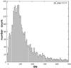Fig. 4 Distribution of the normalized number count of S/N quadrupole.

7. PSF correction

In the previous section we showed the relationship between the 0th-ellipticity and the reduced shear. The 0th-ellipticity is simply the reduced shear if the reduced shear is less than 1 and if there is no PSF effect. We will now account for the PSF effect. In this paper we use the ERA method which is described in Okura & Futamase (2014) in detail, and we briefly outline this method.

7.1. ERA method

We first write the image, which was smeared by PSF from the lensed image, as I^Smd(θ). This image can be described by convolution with the lensed image and PSF P(θ) as $\begin{array}{ccc}\mathit{Î}\mathit{Smd}\mathrm{\left(}{k}\mathrm{\right)}\mathrm{=}\mathit{Î}\mathit{Lnsd}\mathrm{\left(}{k}\mathrm{\right)}\mathit{P̂}\mathrm{\left(}{k}\mathrm{\right)}\mathit{,}& & \end{array}$(37)where the “hat” symbol indicates that a Fourier transform has been performed on the function. We denote the ellipticity of the observed image I^Smd as ${{ϵ}}_{\mathrm{0}\mathrm{th}}^{\mathit{S}}$, and the ellipticity of the lensed image I^Lnsd as ${{ϵ}}_{\mathrm{0}\mathrm{th}}^{\mathit{L}}$. One possible way to obtain ${{ϵ}}_{\mathrm{0}\mathrm{th}}^{\mathit{L}}$ is by deconvolution such as $\begin{array}{ccc}\mathit{Î}\mathit{Lnsd}\mathrm{\left(}{k}\mathrm{\right)}\mathrm{=}\frac{\mathit{Î}\mathit{Smd}\mathrm{\left(}{k}\mathrm{\right)}}{\mathit{P̂}\mathrm{\left(}{k}\mathrm{\right)}}\mathrm{=}\frac{\mathit{Î}\mathit{Smd}\mathrm{\left(}{k}\mathrm{\right)}\mathit{P̂}\mathrm{\ast }\mathrm{\left(}{k}\mathrm{\right)}}{\mathrm{\left|}\mathit{P̂}\mathrm{\right(}{k}\mathrm{)}{\mathrm{|}}^{\mathrm{2}}}\mathrm{·}& & \end{array}$(38)We need to introduce the deconvolution constant C^Dec to avoid dividing by zero, so that $\begin{array}{ccc}\mathit{Î}\mathit{Lnsd}\mathrm{\left(}{k}\mathrm{\right)}\mathrm{=}\frac{\mathit{Î}\mathit{Smd}\mathrm{\left(}{k}\mathrm{\right)}\mathit{P̂}\mathrm{\ast }\mathrm{\left(}{k}\mathrm{\right)}}{\mathrm{\left|}\mathit{P̂}\mathrm{\right(}{k}\mathrm{)}{\mathrm{|}}^{\mathrm{2}}\mathrm{+}{\mathit{C}}^{\mathrm{Dec}}}\mathrm{·}& & \end{array}$(39)Especially in real analysis, a large deconvolution constant is needed owing to pixel noise, which makes a different ellipticity and introduces a systematic error; some samples of the errors from large C^Dec can be seen in Table 1, but the table shows only a tendency introduced by using large C^Dec, and the detailed values of C^Dec do not have any meaning, because it depends on total count of images and so on.

The idea of PSF correction for the 0th-ellipticity is to construct an artificial image I^ESmd, which has ${{ϵ}}_{\mathrm{0}\mathrm{th}}^{\mathit{L}}$ by re-smearing the lensed image using an artificial PSF ${\mathit{P}}^{\mathit{E}}\mathrm{\left(}{\theta }\mathit{,}{{ϵ}}_{\mathrm{0}\mathrm{th}}^{\mathit{L}}\mathrm{\right)}$ with ellipticity ${{ϵ}}_{\mathrm{0}\mathrm{th}}^{\mathit{L}}$ (but an arbitrary profile and size) in such a way that the following relation is satisfied: $\begin{array}{ccc}\mathit{Î}\mathit{ESmd}\mathrm{\left(}{k}\mathrm{\right)}\mathrm{=}\mathit{Î}\mathit{Lnsd}\mathrm{\left(}{k}\mathrm{\right)}\mathit{P̂}\mathit{E}\mathrm{\left(}{k}\mathrm{\right)}\mathrm{=}\mathit{Î}\mathit{Smd}\mathrm{\left(}{k}\mathrm{\right)}\frac{\mathit{P̂}\mathit{E}\mathrm{\left(}{k}\mathrm{\right)}}{\mathit{P̂}\mathrm{\left(}{k}\mathrm{\right)}}\mathrm{·}& & \end{array}$(40)Since I^ESmd also has the ellipticity ${{ϵ}}_{\mathrm{0}\mathrm{th}}^{\mathit{L}}$ by definition, the reduced shear can be obtained by measuring ${{ϵ}}_{\mathrm{0}\mathrm{th}}^{\mathit{ES}}$. In the previous ERA paper, we suggested two possible methods for solving Eq. (40). One is to use the deconvolution constant, which we refer to as Method A. Another is re-smearing the deconvolved image, which we call Method B. In Method B, the artificial PSF is divided as ; then Eq. (40) becomes $\begin{array}{ccc}\mathit{Î}\mathit{ESmd}\mathrm{\left(}{k}\mathrm{\right)}\mathrm{=}\mathit{Î}\mathit{Smd}\mathrm{\left(}{k}\mathrm{\right)}\mathrm{\Delta }\mathit{P̂}\mathrm{\left(}{k}\mathrm{\right)}\mathit{.}& & \end{array}$(41)Both methods require iterations until I^ESmd and P^E have the same ellipticity. We refer to the ERA method of PSF correction applied to the 0th-ellipticity as the 0-ERA method. More details regarding the ERA method can be found in the previous paper.

7.2. Simulation test

We tested a precision PSF correction for the 0th-ellipticity by using a simple simulated image. In real weak lensing analysis, there are many effects that make errors in shear estimation, e.g. PSF effect, pixel noise effect, pixelization, etc. Therefore, we need to study them for precise shear estimation, but many of them are too complex to study at the same time. So in this paper, we consider only simple PSF effects because the ERA method does not use approximations in PSF correction; then, if the results of this simulation have no systematic errors it shows that 0th-ellipticity can be used in the ERA method in the same way as 2nd-ellipticity. The parameters for this simulation are the same as used in Okura & Futamase (2014) which initially described the ERA method.

7.3. Simulation parameters

We used Gaussian and Sérsic galaxy images and a Gaussian PSF image, where the ellipticity of the simulated image ϵ_0th is (0.3, 0.0); the ellipticities of the PSF are [(0.0, 0.0), (0.1, 0.1), (0.3, 0.0), (−0.6, −0.6)]; and the size of the PSF is 0.5, 1.0, and 1.5 times as large as the galaxy. A large size image is used to enable us to neglect pixelization. We then tested the following six cases.

• 1. Deconvolution: standard deconvolution with a deconvolution constant small enough to neglect error from the deconvolution constant discussed in Sect. 3.3. This is not a realistic analysis owing to the pixel noise effect.

• 2. Method A: re-smearing the deconvolved image where the size of P^E is the same as the PSF R^P.

• 3. Method A2: re-smearing the deconvolved image where the size of P^E is 2 times as large as the PSF R^P.

• 4. Method A3: re-smearing the deconvolved image where the size of P^E is 3 times as large as the PSF R^P.

• 5. Method B1: re-smearing the smeared image where size of ΔP is the same as the PSF R^P.

• 6. Method B2: re-smearing the smeared image where the size of ΔP is the same as the size of I^Smd.

Figures 5 to 8 show the PSF corrected ellipticities. Table 2 shows the simulation parameters for each figure set.

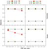Fig. 5 Results of the PSF correction tests with circular PSF. The differences between the four panels are the profile of the galaxy and the analysis method. Top panels are results with Gaussian galaxies and bottom panels are with Sérsic galaxies. Left panels are with methods: red symbols (Dec) indicate PSF correction by deconvolution, green symbols (B1) indicate Method B1, and black symbols (B2) indicate Method B2. Right panels are with methods: red symbols (A1) indicate PSF correction using Method A1, green symbols (A2) indicate use of Method A2, and black symbols (A3) indicate use of Method A3. In each panel, the PSF size ratio (0.5, 1.0, 1.5) is plotted on the horizontal axis and ellipticity with PSF correction is plotted on the vertical axis. Squares indicate ellipticity 1 for which the true value is 0.3, and triangles indicate ellipticity 2 for which the true value is 0.0.

Fig. 6 Same as Fig. 5, but PSF has ellipticity (0.1, 0.1).

Fig. 7 Same as Fig. 5, but PSF has ellipticity (0.3, 0.0).

Fig. 8 Same as Fig. 5, but PSF has ellipticity (−0.6, −0.6).

Figures 5 and 6 show the results using a circular or small elliptical (0.1, 0.1) PSF. These results show that the deconvolution method cannot correct the PSF, but the 0-ERA method can correct a small elliptical PSF with no systematic error (where no systematic error means that the systematic error is under 0.1%). Figure 7 shows the cases with an intermediate elliptical PSF. It can be seen that the 0-ERA method can correct the PSF, because the ERA method is formulated in such a way that the PSF has the same ellipticity with the objects. Figure 8 shows the results with a large elliptical PSF. These results show that the 0-ERA method can correct the PSF with no systematic error if appropriate parameters are chosen for the re-smearing function. Similar results were obtained using the ERA method (2nd-ellipticity), which can be seen in the previous paper describing ERA. Thus, the 0-ERA method can analyse weak lensing shear with an accuracy similar to the ERA method.

Table 3 is the PSF corrected ellipticities of the simulation with circular PSF.

8. Conclusions and comments

We developed a new method of weak lensing analysis by defining a new ellipticity that is defined from 0th order moments.

This ellipticity is measured in the region near the centre, rather than the usual ellipticity which is defined from the quadrupole moments. Therefore, the new ellipticity has a higher S/N than that of quadrupole ellipticity, and it is expected that this new method can measure weak gravitational shear with higher accuracy. The gain in the S/N is about $\sqrt{\mathrm{2}}\mathrm{~}\sqrt{\mathrm{3}}$ if the image is an elliptical Gaussian. We measured the 0th-ellipticities and S/N using objects from Abell 1689, and showed that the 0th- and 2nd-ellipticities have a high correlation. The gain in S/N using real data is almost the same as when using a simple elliptical Gaussian image and the gain in the number count using the 0th-ellipticity is about 1.5 ~ 2. As a result, objects that are fainter can be used in this new weak gravitational lensing shear analysis, and therefore more accurate shear analysis is expected. The mass reconstruction for galaxy clusters using this scheme will be evaluated in forthcoming papers.

We tested the PSF correction using this method in a simple simulation, and the results of the simulation show that this new method is able to correct the PSF effect with enough accuracy by using an appropriate re-smearing function. In this simulation, we used a large image to neglect the noise from pixelization, and therefore this test is not realistic. We also did not consider pixel noise and the interpolation problem in PSF correction. We succeeded in correcting PSF correction without any systematic error, but there are still many issues for precise weak lensing analysis in real situations, for examples in correcting complex PSF, PSF interpolation, stacking image, pixel noise, pixelization, and so on. For example, we studied pixel noise effects on measuring ellipticity in Okura & Futamase (2013), but the pixel noise effect correction with PSF correction is very important for precise weak lensing analysis. All of these issues are very important and complicated problems, and thus need to be studied individually. The detailed evaluation of the systematic errors will be done in future studies.

Acknowledgments

We would like to thank Alan T. Lefor for improving the English usage in this paper.

References

Appendix A: Ellipticity of the 0th order moment and the reduced shear

In this Appendix, we show detailed calculations for deriving the relation between the 0th-ellipticity and the reduced shear, and how to use the 0th-ellipticities e_0th and ϵ_0th.

Since the zero image has circular image, the following equations are obtained, 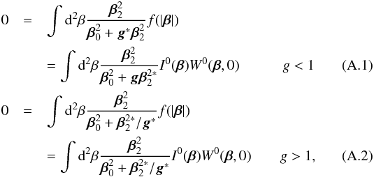$\begin{array}{ccc}\mathrm{0}& \mathrm{=}& \int {\mathrm{d}}^{\mathrm{2}}\mathit{\beta }\frac{{{\beta }}_{\mathrm{2}}^{\mathrm{2}}}{{{\beta }}_{\mathrm{0}}^{\mathrm{2}}\mathrm{+}{{g}}^{\mathrm{\ast }}{{\beta }}_{\mathrm{2}}^{\mathrm{2}}}\mathit{f}\mathrm{\left(}\mathrm{\right|}{\beta }\mathrm{\left|}\mathrm{\right)}\\ & & \mathrm{=}\mathrm{\int }{\mathrm{d}}^{\mathrm{2}}\mathit{\beta }\frac{{{\beta }}_{\mathrm{2}}^{\mathrm{2}}}{{{\beta }}_{\mathrm{0}}^{\mathrm{2}}\mathrm{+}{g}{{\beta }}_{\mathrm{2}}^{\mathrm{2}\mathrm{\ast }}}{\mathit{I}}^{\mathrm{0}}\mathrm{\left(}{\beta }\mathrm{\right)}{\mathit{W}}^{\mathrm{0}}\mathrm{\left(}{\beta }\mathit{,}\mathrm{0}\mathrm{\right)}\mathit{g}\mathit{<}\mathrm{1}\\ \mathrm{0}& \mathrm{=}& \int {\mathrm{d}}^{\mathrm{2}}\mathit{\beta }\frac{{{\beta }}_{\mathrm{2}}^{\mathrm{2}}}{{{\beta }}_{\mathrm{0}}^{\mathrm{2}}\mathrm{+}{{\beta }}_{\mathrm{2}}^{\mathrm{2}\mathrm{\ast }}\mathit{/}{{g}}^{\mathrm{\ast }}}\mathit{f}\mathrm{\left(}\mathrm{\right|}{\beta }\mathrm{\left|}\mathrm{\right)}\\ & & \mathrm{=}\mathrm{\int }{\mathrm{d}}^{\mathrm{2}}\mathit{\beta }\frac{{{\beta }}_{\mathrm{2}}^{\mathrm{2}}}{{{\beta }}_{\mathrm{0}}^{\mathrm{2}}\mathrm{+}{{\beta }}_{\mathrm{2}}^{\mathrm{2}\mathrm{\ast }}\mathit{/}{{g}}^{\mathrm{\ast }}}{\mathit{I}}^{\mathrm{0}}\mathrm{\left(}{\beta }\mathrm{\right)}{\mathit{W}}^{\mathrm{0}}\mathrm{\left(}{\beta }\mathit{,}\mathrm{0}\mathrm{\right)}\mathit{g}\mathit{>}\mathrm{1}\mathit{,}\end{array}$where f is an arbitrary function, and W⁰ is a Gaussian weight function, which is a function of the absolute value of β and the following approximation: $\begin{array}{ccc}{\mathit{I}}^{\mathrm{0}}\mathrm{\left(}{\beta }\mathrm{\right)}& \mathrm{\approx }& {\mathit{I}}^{\mathrm{0}}\mathrm{\left(}\mathrm{\right|}{\beta }\mathrm{\left|}\mathrm{\right)}\mathit{.}\end{array}$(A.3)In the image plane, these functions are written as $\begin{array}{ccc}& & \frac{{{\beta }}_{\mathrm{2}}^{\mathrm{2}}}{{{\beta }}_{\mathrm{0}}^{\mathrm{2}}\mathrm{+}{{g}}^{\mathrm{\ast }}{{\beta }}_{\mathrm{2}}^{\mathrm{2}}}\mathrm{=}\frac{{{\beta }}_{\mathrm{1}}^{\mathrm{1}}}{{{\beta }}_{\mathrm{1}}^{\mathrm{1}\mathrm{\ast }}\mathrm{+}{{g}}^{\mathrm{\ast }}{\beta }}\mathrm{\propto }\frac{{{\theta }}_{\mathrm{1}}^{\mathrm{1}}\mathrm{-}{g}{{\theta }}_{\mathrm{1}}^{\mathrm{1}\mathrm{\ast }}}{{{\theta }}_{\mathrm{1}}^{\mathrm{1}\mathrm{\ast }}}\mathrm{=}\frac{{{\theta }}_{\mathrm{2}}^{\mathrm{2}}}{{{\theta }}_{\mathrm{0}}^{\mathrm{2}}}\mathrm{-}{g} \\ & & \frac{{{\beta }}_{\mathrm{2}}^{\mathrm{2}}}{{{\beta }}_{\mathrm{0}}^{\mathrm{2}}\mathrm{+}{{\beta }}_{\mathrm{2}}^{\mathrm{2}}\mathit{/}{g}}\mathrm{=}\frac{{{\beta }}_{\mathrm{1}}^{\mathrm{1}}}{{{\beta }}_{\mathrm{1}}^{\mathrm{1}\mathrm{\ast }}\mathrm{+}{{\beta }}_{\mathrm{1}}^{\mathrm{1}}\mathit{/}{g}}\mathrm{\propto }\frac{\mathrm{1}}{{g}}\frac{{{\theta }}_{\mathrm{1}}^{\mathrm{1}}\mathrm{-}{{\theta }}_{\mathrm{1}}^{\mathrm{1}\mathrm{\ast }}\mathit{/}{g}}{{{\theta }}_{\mathrm{1}}^{\mathrm{1}}}\mathrm{=}{{g}}^{\mathrm{2}}\left(\frac{\mathrm{1}}{{g}}\mathrm{-}\frac{{{\theta }}_{\mathrm{2}}^{\mathrm{2}\mathrm{\ast }}}{{{\theta }}_{\mathrm{0}}^{\mathrm{2}}}\right) \\ & & {\mathit{I}}^{\mathrm{0}}\mathrm{\left(}{\beta }\mathrm{\right)}\mathrm{=}{\mathit{I}}^{\mathit{Lnsd}}\mathrm{\left(}{\theta }\mathrm{\right)}\end{array}$

$\begin{array}{ccc}{\mathit{W}}^{\mathrm{0}}\mathrm{\left(}{\beta }\mathit{,}\mathrm{0}\mathrm{\right)}& \mathrm{=}& \exp \left(\mathrm{-}\frac{{{\beta }}_{\mathrm{0}}^{\mathrm{2}}}{{\mathit{\sigma }}_{\mathrm{0}}^{\mathrm{2}}}\right)\mathrm{=}\exp \left(\mathrm{-}\frac{{{\theta }}_{\mathrm{0}}^{\mathrm{2}}\mathrm{-}\mathrm{Re}\left[\frac{\mathrm{2}{g}}{\mathrm{1}\mathrm{+}\mathrm{|}{g}{\mathrm{|}}^{\mathrm{2}}}{{\theta }}_{\mathrm{2}}^{\mathrm{2}\mathrm{\ast }}\right]}{{\mathit{\sigma }}^{\mathrm{2}}}\right)\\ & \mathrm{=}& \exp \left(\mathrm{-}\frac{{{\theta }}_{\mathrm{0}}^{\mathrm{2}}\mathrm{-}\mathrm{Re}\mathrm{[}{{\delta }}^{\mathrm{\ast }}{{{\theta }}_{\mathrm{2}}^{\mathrm{2}}}^{\mathrm{]}}}{{\mathit{\sigma }}^{\mathrm{2}}}\right)\mathrm{=}\mathit{W}\mathrm{\left(}{\theta }\mathit{,}{\delta }\mathrm{\right)}\mathrm{=}\mathit{W}\mathrm{\left(}{\theta }\mathit{,}{{ϵ}}_{\mathit{W}}\mathrm{\right)}\mathit{,}\end{array}$(A.7)where we temporarily set ϵ_W = δ. Therefore, in the source plane Eqs. (A.1) and (A.2) change to $\begin{array}{ccc}\mathrm{0}& \mathrm{=}& \int {\mathrm{d}}^{\mathrm{2}}\mathit{\theta }\left(\frac{{{\theta }}_{\mathrm{2}}^{\mathrm{2}}}{{{\theta }}_{\mathrm{0}}^{\mathrm{2}}}\mathrm{-}{g}\right){\mathit{I}}^{\mathit{Lnsd}}\mathrm{\left(}{\theta }\mathrm{\right)}\mathit{W}\mathrm{\left(}{\theta }\mathit{,}{\delta }\mathrm{\right)}\mathrm{=}{\mathrm{[}{\mathrm{𝒵}}_{\mathrm{2}}^{\mathrm{0}}\mathrm{-}{g}{{\mathrm{𝒵}}_{\mathrm{0}}^{\mathrm{0}}}^{\mathrm{]}}}_{\mathrm{\left(}{\mathit{I}}^{\mathit{Lnsd}}\mathit{,}{\delta }\mathrm{\right)}}\\ & & \mathit{g}\mathit{<}\mathrm{1}\\ \mathrm{0}& \mathrm{=}& \int {\mathrm{d}}^{\mathrm{2}}\mathit{\theta }\left(\frac{{{\theta }}_{\mathrm{2}}^{\mathrm{2}}}{{{\theta }}_{\mathrm{0}}^{\mathrm{2}}}\mathrm{-}\mathrm{1}\mathit{/}{{g}}^{\mathrm{\ast }}\right){\mathit{I}}^{\mathit{Lnsd}}\mathrm{\left(}{\theta }\mathrm{\right)}\mathit{W}\mathrm{\left(}{\theta }\mathit{,}{\delta }\mathrm{\right)}\mathrm{=}{\mathrm{[}{\mathrm{𝒵}}_{\mathrm{2}}^{\mathrm{0}}\mathrm{-}{\mathrm{𝒵}}_{\mathrm{0}}^{\mathrm{0}}\mathit{/}{{g}}^{\mathrm{\ast }}\mathrm{]}}_{\mathrm{\left(}{\mathit{I}}^{\mathit{Lnsd}}\mathit{,}{\delta }\mathrm{\right)}}\\ & & \mathit{g}\mathit{>}\mathrm{1}\mathit{,}\end{array}$and finally we obtain $\begin{array}{ccc}{\left(\frac{{\mathrm{𝒵}}_{\mathrm{2}}^{\mathrm{0}}}{{\mathrm{𝒵}}_{\mathrm{0}}^{\mathrm{0}}}\right)}_{\mathrm{\left(}{\mathit{I}}^{\mathit{Lnsd}}\mathit{,}{\delta }\mathrm{\right)}}& \mathrm{\equiv }{{e}}_{\mathrm{0}\mathrm{th}}& \mathrm{=}{g}\mathit{g}\mathit{<}\mathrm{1}\\ {\left(\frac{{\mathrm{𝒵}}_{\mathrm{2}}^{\mathrm{0}}}{{\mathrm{𝒵}}_{\mathrm{0}}^{\mathrm{0}}}\right)}_{\mathrm{\left(}{\mathit{I}}^{\mathit{Lnsd}}\mathit{,}{\delta }\mathrm{\right)}}& \mathrm{\equiv }{{e}}_{\mathrm{0}\mathrm{th}}& \mathrm{=}\frac{\mathrm{1}}{{{g}}^{\mathrm{\ast }}}\mathit{g}\mathit{>}\mathrm{1.}\end{array}$Then ϵ_W is derived as $\begin{array}{ccc}{{ϵ}}_{\mathit{W}}\mathrm{=}{\delta }\mathrm{=}\frac{\mathrm{2}{g}}{\mathrm{1}\mathrm{+}\mathrm{|}{g}{\mathrm{|}}^{\mathrm{2}}}\mathrm{=}\frac{\mathrm{2}{{e}}_{\mathrm{0}\mathrm{th}}}{\mathrm{1}\mathrm{+}\mathrm{|}{{e}}_{\mathrm{0}\mathrm{th}}{\mathrm{|}}^{\mathrm{2}}}\mathrm{\equiv }{{ϵ}}_{\mathrm{0}\mathrm{th}}\mathit{.}& & \end{array}$(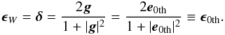A.12)

All Tables

All Figures

	Fig. 1 Correlation between 0th- and 2nd-epsilon values measured from real data.
In the text

	Fig. 2 Epsilon vs. S/N measured from real data.
In the text

	Fig. 3 Distribution of the normalized number count of S/N monopole.
In the text

	Fig. 4 Distribution of the normalized number count of S/N quadrupole.
In the text

Fig. 5 Results of the PSF correction tests with circular PSF. The differences between the four panels are the profile of the galaxy and the analysis method. Top panels are results with Gaussian galaxies and bottom panels are with Sérsic galaxies. Left panels are with methods: red symbols (Dec) indicate PSF correction by deconvolution, green symbols (B1) indicate Method B1, and black symbols (B2) indicate Method B2. Right panels are with methods: red symbols (A1) indicate PSF correction using Method A1, green symbols (A2) indicate use of Method A2, and black symbols (A3) indicate use of Method A3. In each panel, the PSF size ratio (0.5, 1.0, 1.5) is plotted on the horizontal axis and ellipticity with PSF correction is plotted on the vertical axis. Squares indicate ellipticity 1 for which the true value is 0.3, and triangles indicate ellipticity 2 for which the true value is 0.0.

In the text

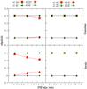	Fig. 6 Same as Fig. 5, but PSF has ellipticity (0.1, 0.1).
In the text

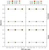	Fig. 7 Same as Fig. 5, but PSF has ellipticity (0.3, 0.0).
In the text

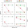	Fig. 8 Same as Fig. 5, but PSF has ellipticity (−0.6, −0.6).
In the text

References

- Bacon, D. J., Refregier, A. R., & Ellis, R. S. 2000, MNRAS, 318, 625 [NASA ADS] [CrossRef] [Google Scholar]
- Bacon, D. J., Massey, R. J., Refregier, A. R., & Ellis, R. S. 2003, MNRAS, 344, 673 [NASA ADS] [CrossRef] [Google Scholar]
- Bernstein, G. M., & Jarvis, M. 2002, AJ, 123, 583 [NASA ADS] [CrossRef] [Google Scholar]
- Bridle, S., Balan, S. T., Bethge, M., et al. 2010, MNRAS, 405, 2044 [NASA ADS] [Google Scholar]
- Casertano, S., Ratnatunga, K. U., & Griffiths, R. E. 2003, ApJ, 598, L71 [NASA ADS] [CrossRef] [Google Scholar]
- Hamana, T., Miyazaki, S., Shimasaku, K., et al. 2003, ApJ, 597, 98 [NASA ADS] [CrossRef] [Google Scholar]
- Heymans, C., Van Waerbeke, L., Bacon, D., et al. 2006, MNRAS, 368, 1323 [NASA ADS] [CrossRef] [Google Scholar]
- Hoekstra, H., Mellier, Y., van Waerbeke, L., et al. 2006, ApJ, 647, 116 [NASA ADS] [CrossRef] [Google Scholar]
- Kaiser, N., Squires, G., & Broadhurst, T. 1995, ApJ, 449, 460 [NASA ADS] [CrossRef] [Google Scholar]
- Kitching, T. D., Miller, L., Heymans, C. E., van Waerbeke, L., & Heavens, A. F. 2008, MNRAS, 390, 149 [NASA ADS] [CrossRef] [Google Scholar]
- Kitching, T. D., Balan, S. T., Bridle, S., et al. 2012, MNRAS, 423, 3163 [NASA ADS] [CrossRef] [Google Scholar]
- Kuijken, K. 2006, A&A, 456, 827 [NASA ADS] [CrossRef] [EDP Sciences] [Google Scholar]
- Maoli, R., van Waerbeke, L., Mellier, Y., et al. 2001, A&A, 368, 766 [NASA ADS] [CrossRef] [EDP Sciences] [Google Scholar]
- Massey, R., Refregier, A., Bacon, D. J., Ellis, R., & Brown, M. L. 2005, MNRAS, 359, 1277 [NASA ADS] [CrossRef] [Google Scholar]
- Massey, R., Heymans, C., Bergé, J., et al. 2007, MNRAS, 376, 13 [NASA ADS] [CrossRef] [Google Scholar]
- Melchior, P. 2011, MNRAS, 412, 1552 [NASA ADS] [CrossRef] [Google Scholar]
- Mellier, Y. 1999, Ann. Rev. Astron. Astrophys., 37, 127 [Google Scholar]
- Miller, L., Egan, M. P., Price, S. D., & Kraemer, K. E. 2007, MNRAS, 382, 315 [NASA ADS] [CrossRef] [Google Scholar]
- Munshi, D., Valagesas, P., Van Waerbeke, L., & Heavens, A. 2008, Phys. Rep., 462, 67 [NASA ADS] [CrossRef] [Google Scholar]
- Okura, Y., & Futamase, T. 2011, ApJ, 730, 9 [NASA ADS] [CrossRef] [Google Scholar]
- Okura, Y., & Futamase, T. 2012, ApJ, 748, 112 [NASA ADS] [CrossRef] [Google Scholar]
- Okura, Y., & Futamase, T. 2013, ApJ, 771, 37 [NASA ADS] [CrossRef] [Google Scholar]
- Okura, Y., & Futamase, T. 2014, ApJ, 792, 104 [NASA ADS] [CrossRef] [Google Scholar]
- Refregier, A. 2003, MNRAS, 338, 35 [NASA ADS] [CrossRef] [Google Scholar]
- Refregier, A., Rhodes, J., & Groth, E. J. 2002, ApJ, 572, L131 [NASA ADS] [CrossRef] [Google Scholar]
- Schneider, P. 2006, in Gravitational lensing: strong, weak and micro (Part 1), Swiss Society for Astrophysics and Astronomy, Saas-Fee Adv. Course, 33, 1 [Google Scholar]
- van Waerbeke, L., Mellier, Y., & Hoekstra, H. 2005, A&A, 429, 75 [NASA ADS] [CrossRef] [EDP Sciences] [Google Scholar]